How To Calculate The Volailiy Of A Sock Marke

on the US stock market

Jean-Gabriel Cousina, Tanguy de Launoisb*

a

ESA, Université de Lille II, France b

FNRS Fellow at the Université catholique de Louvain, Belgium

ABSTRACT

The relation between information flow and asset prices behavior is one of the key issues of modern finance. Our study investigates more closely the link between frequency of information arrivals and stock return volatility. It aims precisely to test empirically the mixture of distribution hypothesis and to check whether the stock returns distribution is driven by the frequencies of information arrivals on the US market. We analyze the impact of news on volatility at the firm-level. We opt for a model with two (Markov switching) regimes of volatility that we apply to all stocks belonging to the S&P 500 index from May 1998 to December 2003. We exploit the panel structure of our data and we find a positive and significant but marginally decreasing impact of the daily frequency of information arrivals on the probability to be in a state of high volatility for the 458 companies considered. Subsequent tests allow us to conclude that this impact crucially depends on the timing and the topic of the news release. Interestingly, news announcing stronger public intervention increases the uncertainty the most, whereas announcements about future privatization lead to the strongest reduction in the stock volatility. We finally perform a cross-sectional regression of the transition probabilities on different measures of news intensity, regularity and persistence. We find a positive relation between the transition probabilities and these characteristics of information. JEL codes: G14

EFA Classification Code: ME

Keywords: News, (conditional) Volatility, Public information arrivals, Mixture of distribution hypothesis, Communication intensity, Markov Switching Regression Model.

* Corresponding author: Other author :

1, Place des Doyens 1 1 Place Déliot

1348 Louvain-la-Neuve 59000 Lille

Belgium France

e-mail address: [email protected] e-mail address: [email protected] We are grateful to Jacques Chardon and Factiva for having offered access to their data base. We especially wish to thank E. de Bodt for his guidance and advice. All errors remain ours.

The relation between information flow and asset prices behavior is one of the key issues of modern finance. How, why and under which conditions do financial news impact stock price volatility, count among the classical (and still debatable) questions in this research area. The clear knowledge and the good understanding of such important issues are of first importance for listed companies. The behavior of stock prices around profit warning announcements is a typical (and probably extreme) example of these phenomena. Carl-Henric Svanberg, Ericsson Chief Executive, still probably remembers the disastrous consequences of his injudicious profit warning of October 16, 2007. At first sight, the news release looked quite innocent: it said that Ericsson’s operating earnings dropped 36% to 5.6bn Swedish crowns ($876m), from 8.8bn crowns a year ago. The problem was that analysts had been expecting earnings of about 8.9bn crowns for the quarter. The market showed no mercy: shares of the company lost 24% in one day, involving that not less than €15.7 billion of Ericsson’s market capitalization vanished in a couple of hours. "This is a day to be humble, concerned and disappointed," said Svanberg during a Webcast press conference in the morning. "This is a dynamic business environment... We should have talked more about it and understood more about it. We have underestimated the impact" of changes in the market, added the CEO1.

That kind of news hardly makes only one victim. Sector spill over effects of such announcements have been quite common. On September 16, 2004, after Celestica, a large-cap electronics manufacturer, cut its outlook for the third quarter, the whole sector of makers of electric parts and equipment as well as providers of related services dropped: Power-One tumbled 6.4%, Plexus fell 5.4%, Littlefuse shed 3.3% and

Benchmark Electronics lost 10% on the New York Stock Exchange. The communications-technology sector was affected the same way, since Stratex Networks dropped 4.4%, Mindspeed Technologies lost 3.3% and MRV Communications fell 3.2%. Financial communication may thus strongly impact stock return, volume and volatility of any company. Such a point deserves to be studied and analyzed carefully. Our primary objective is to investigate the relation between public information and stock volatility. To what extent does the discontinuous frequency of news releases affect the volatility of the daily stock returns? And what are the factors strengthening or weakening this relation? These are precisely the main questions that we aim to answer in this paper. They are crucial from both a practical and an academic perspective, since recent academic works have put into light the importance of developing a better understanding of the determinants of return volatility. Easley and O’Hara (2001) bring some evidence that the less transparent and disclosing a company is, the higher its cost of capital will be. Such a conclusion already offers some insight of how significant the influence of news releases (in quality and in quantity) on stock prices can be. Campbell, Lettau, Malkiel and Xu (2001) find that the proportion of firm-specific variance in the total stock variance has steadily been increasing for the last thirty years and thus provides us with another good reason to investigate the relation between firm-specific news and idiosyncratic volatility. As a matter of fact, one may wonder whether the regular increase in idiosyncratic variance detected by Campbell and al. (2001) could possibly be linked with the obvious contemporaneous increase in the financial communication intensity. Our results seem to support such an assertion. Eventually, Goyal and Santa Clara (2002) detect a positive relation between idiosyncratic variance and expected stock return. For idiosyncratic risk is not perfectly diversifiable and 1

Sources: lightreading :http://www.lightreading.com/document.asp?doc_id=136368, BBC news: http://news.bbc.co.uk/1/hi/business/7046703.stm and the Guardian:

investors are assumed risk-averse, an increase in the firm-specific part of the stock volatility can induce an increase in the cost of capital2.

Since we focus on the stock volatility, an adequate model of its dynamics is obviously of prime importance. If GARCH models count undoubtedly among the most famous conditional volatility models, alternative frameworks exist and deserve to be considered. The Markov switching regression (MSR) approach is one of them: this rather original approach avoids the classical drawbacks of the GARCH models and allows us to indirectly test the Mixture of Distribution Hypothesis (MDH), which argues that the stock volatility is directly related to the information frequency.

Although GARCH and MSR models give useful and quite reliable estimates of the conditional stock variance, they still remain reduced form models not dedicated to explain observed changes in stock volatility and to point out the core factors driving its behavior. In our quest for an innovative explicative model of the stock volatility, the MDH may well be of great help, since it suggests explicitly that the stock volatility is closely linked to the information frequency. Therefore it largely justifies the introduction of the “daily number of press releases on a stock” as the most appropriate explanatory variable in the basic equation of our intended explicative model.

With regard to the existing literature, our contributions are of three kinds: they concern the data used as well as the methodology adopted and the results obtained.

In order to test empirically whether information flows drive stock return volatility, we apply our econometrical model to all stocks pertaining to the S&P 500 index from May 13, 1998 to December 31, 20033. CRSP-tapes provide us with the series of daily stock

2

However, this point remains controversial. In obvious contradiction with Goyal and Santa Clara (2002), Wei and Zhang (2004) claim that idiosyncratic risk does not matter.

3

In a previous work (see Cousin and de Launois (2006)), we had conducted the same kind of analysis on the French market, i.e. on all stocks members of the CAC 40 index between January 1999 and December 2003.

prices, while Factiva gives us access to a particularly rich and advantageous news sample composed of all time-stamped societal and industrial Reuters and Dow Jones news releases concerning all companies selected above. This kind of financial communication counts undoubtedly among the most up to date and relevant public information that investors can collect when trading on the market. Furthermore, since we are only interested in the impact of information intensity on the idiosyncratic stock variance, we restrict our investigation to firm-specific and industrial-specific news and chose not to introduce any market or macroeconomic news in the sample (as it will be explained below, we will control for possible market and macroeconomic shocks on stock variance through controlling for the market variance in the regression equation). Finally, for we want to test the link between the daily number of firm-specific news releases and the corresponding stock volatility, it is necessary to know which company (or companies) is (or are) concerned by each news release. Our sample provides us with such an interesting item, among many others. It allows us to refine the classical aggregate market-level analysis into a more subtle and accurate firm by firm study. Our methodology differs in many respects from the previous studies on the topic mentioned in Section 2. We analyze the impact of news on volatility at the firm-level, i.e. company by company, and not at the market-level, i.e. impact of news on the index. It allows us to capture the entire “firm-specific effect” contained in the news which is obviously lost at the aggregate level. We also employ conditional volatility measures (instead of unconditional volatility measures) in order to take the volatility persistence effect into account. We first replicate on a daily basis the GARCH approach of Kalev, Liu, Pham and Jarnecic (2004) with our specific data set at the firm-level. We then opt for a market model with two (Markov switching) regimes of volatility, which is more robust and general than the GARCH model used by Kalev and al. (2004) because it needs less strong assumptions on the conditional volatility process. Moreover, such a

MSR model allows us to explicitly take advantage of the central Roll (1988)’s idea4 of a mixed return distribution (“with news” and “no news”) driven by news arrivals and to test the relevance of such an intuition. The subsequent econometric methodology consists basically of two steps: estimating the daily probabilities of being in a high volatility state thanks to the developed two-state market model and regressing in a panel framework these obtained probabilities on some possibly explicative variables (like the daily number of news wires) in order to understand the determinants driving the stock returns volatility. Like Kalev and al. (2004), we control for the daily volume of trades, a possible proxy of private information, and we find it to be significant. Unlike Kalev and al. (2004), we control for factors such as the market conditional volatility and the sector conditional volatility, which turn out to be highly significant. Furthermore, we control for possible time effects, both alone and in interaction with our news variables. Only the first type of time effects appears to be significant. We also choose to perform the same regressions on different news subsets selected on the basis of various criteria, like the subject or the timing of the news release. In a last analysis, we investigate impact of various characteristics of the company (the intensity, regularity and persistence of the communication, as well as the size of the company) on the probabilities of transition from one regime (low or high) to another regime of volatility (low or high).

Our main finding is that public information flows strongly affect the stock returns distribution. In the GARCH framework, our results are consistent with those of Kalev and al. (2004). The news frequency seems to be largely responsible for the persistence volatility effect, and its impact on the volatility level is substantial. In the MSR model framework, we find a positive and significant impact of the daily frequency of information arrivals on the probability to be in a state of high volatility for each of the 458 companies considered. Moreover, we observe that this impact is marginally

4

decreasing. The regressions on various data subsets offer very interesting results: news released during trading hours seems to have a much stronger impact than news released during non-trading hours. In terms of subject, with a coefficient of 0.32, press releases concerning earnings surprises appear to have the greatest impact on the stock volatility. This confirms us in the common view that investors do not like being surprised at all. Other kinds of news, in particular Regulation and government policy and earnings projections (especially the subset of analyst comments and recommendations) present much more moderate positive impacts (with a coefficient around 0.05), but still very significant. Interestingly, news announcing stronger public intervention increases the uncertainty the most (after the earnings surprises category), whereas announcements about future privatization lead to the strongest reduction in the stock volatility. We finally end this study with cross-sectional regressions of the transition probabilities on different measures of news intensity, regularity and persistence. We find a positive relation between the transition probabilities and these characteristics of information. The more frequently and regularly information is released, the higher the transition probabilities. And the impact is stronger on the transition probability from the low to the high volatility regime than the other (high to low).

Our paper is organized as follows. Section 2 provides a brief review of the literature about the relation between information and conditional volatility. Section 3 describes the used data sets: stock prices and Reuters and Dow Jones news wires. Section 4 presents the GARCH and the Markov switching regimes models used in the subsequent empirical part. Section 5 displays and comments results. Section 6 concludes and provides some perspectives for future research.

2

Information and conditional volatility

2.1

Modeling the conditional volatility

In the literature, the time-varying nature of the volatility is a well-known empirical fact. Presence of conditional heteroscedasticity is well documented in most financial time-series. As a natural consequence, several authors have tried to account for this volatility persistence effect in alternative econometric frameworks like ARCH (see Engle (1982)) and GARCH5 (see Bollerslev (1988)) approaches. By expressing the stock idiosyncratic variance at time t as a linear function of the past stock idiosyncratic variances and innovations (at t-1, t-2, etc.), these models provide conditional estimates of the stock volatility while taking the persistence volatility effect into account. Markov switching regression models (MSR) appear as another interesting way to capture conditional heteroscedasticity evolutions. In such a non-linear dynamic framework, stock returns distribution is supposed to switch from a low to a high volatility regime (and vice-versa) according to some fixed transition probabilities. MSR models exhibit a more general structure than the GARCH models, since they impose fewer assumptions on the functional form of the conditional volatility. Moreover, GARCH models may sometimes present some annoying convergence problems, while MSR models are generally more reliable in this respect. Eventually, GARCH models do not rest on a clear theoretical justification (they are sort of reduced form models), whereas MSR models are implicitly based upon such a powerful argument, which is known as the Mixture of Distribution Hypothesis (MDH). Suggested for the first time by Clark (1973), it posits that the joint distribution of daily return and volume can be modeled as a mixture of bivariate normal distributions. Specifically, they are contemporaneously dependent on an underlying mixing variable that represents the flow of information. As

5

ARCH and GARCH stand respectively for autoregressive conditional heteroscedasticity and generalized autoregressive conditional heteroscedasticity (models).

a consequence, the variance of returns at a given interval is expected to be proportional to the rate of information arrival at the market. About fifteen years later, Roll (1988) shows empirically that the sample variance and the kurtosis for example can reveal something about the probability of information and the difference between the information-related distribution and the non-information-related distribution of returns, which is totally consistent with the MDH. One year later, Ross (1989) brings some convincing theoretical evidence supporting the MDH and demonstrates that in an arbitrage-free economy, the volatility of prices is directly related to the rate of flow of information to the market. An avowed objective of our study is precisely to test empirically that mixture of distribution hypothesis and to check whether the stock returns distribution is driven by the frequency of information arrivals on the Paris stock Exchange (Euronext).

In this context, the MSR model turns out to be the most suitable specification, since it is the closest translation of the mixture of distribution hypothesis into an empirical estimation. Chauvet and Hamilton (2005) shows that a simple Markov switching model fits particularly well the data when these are suspected to follow a mixture of distributions. In our case, Davies’s test confirms that a Markov switching model with two regimes must be preferred to a simple market model. We could consider more than two regimes, but in absence of strong and annoying outliers, the addition of a third regime does not bring anything valuable and will only increase the complexity of the model.

2.2

News arrivals and market reactions

If many authors tried to establish the reality of the positive relation between flows of information and stock (or market) volatility, the empirical evidence of such a positive relation is everything but overwhelming, probably because of the difficulty to find good

empirical proxy of information arrivals and of the poor volatility estimates that were traditionally used. The difficulty to precisely measure information arrivals appears in the variety of proxies employed by previous empirical studies on the topic. Berry and Howe (1993) use the number of daily newspaper headlines and earnings announcements and Ederington and Lee (1993) investigate the importance of macroeconomic news, whereas Mitchell and Mulherin (1994) employ the number of specific stock market announcements in order to test the impact of the rate of information on the market volatility. « However, the use of unconditional volatility measures such as absolute daily market returns in these studies often generates weak or inconclusive results regarding the news–volatility relation »6. Indeed, such a proxy is known to be quite noisy, and the presence of conditional heteroscedasticity in the returns time-series may significantly alter the quality of the results. It is precisely to account for this well-known phenomenon of conditional heteroscedasticity that Kalev and al. (2004) choose to test the relation between firm-specific announcements (as a proxy for information flows) and volatility on the Australian Stock Exchange in a GARCH framework. Their analysis reveals a positive and significant impact of the arrival rate of the selected news variable on the conditional variance of stock returns, even after controlling for the potential effects of trading volume and high opening volatility. They find the respective coefficients of these two last control variables to be positive and significant, except on a daily basis. Eventually, they split all their press releases into different categories according to their subject, since Andersen (1996) argues that different types of news have different stochastic arrival processes, so that we may legitimately expect them to have a different impact on the conditional stock volatility.

It is worth noticing that some authors have worked specifically on the French market, like Lardic and Mignon (2003) and Lespagnol and Teïteltche (2005), as we did in a previous study (Cousin and de Launois (2006)).

3

Sample selection

Our final sample covers a period ranging from May 13, 1998 to December 31, 2003 (i.e. 1418 trading days). Our firms’ universe is composed of the 458 US stocks that were part of the S&P 500 index in May 2006 and which survived the filtering process. We have indeed deleted all stocks (i.e. 42) that were acquired, merged or that have purely vanished over the selected period, as well as stocks with insufficient news or financial data. We do not consider news prior to May 13, 1998, because the time of arrival of news is a relatively new feature of Factiva and was not systematically provided before this date. As this item appears to be useful in the aggregation process of announcements and the subsequent regressions, and since we wish to work on a dataset as homogenous as possible, we decide to restrict our attention to this specific time range, as well as to 458 companies out of the 500 initially considered, for some necessary data lack for 42 of them.

Eventually, we are left with a broad and representative sample of the US market since it accounts for not less than 75% of the US market value. The average total market value of our sample is $25,000.489 billion. The mean (median) company market value is $55.653 billion ($2.175 billion). For all firms included in this sample, we use daily closing prices from May 13, 1998 to December 31, 2003. The three largest sectors in the sample are the commercial banking (5,8%), Electricity/Gas Utilities (3,8%) and Semiconductors (3,4%). We use as a market portfolio the CRSP EW. The data are obtained from the CRSP-tapes.

All press releases were collected through the Factiva data base web site7. Factiva is a Dow Jones and Reuters company that provides professionals with business news and information sources like The Wall Street Journal or The Financial Times for example. Our sample is composed of all corporate and industrial news wires concerning firms included in the S&P 500 index and recorded by Dow Jones and Reuters from May 13, 1998 to December 31, 2003. Dow Jones and Reuters news wires are the two major sources of news available in Factiva and are of course redundant. We have performed the whole analysis with each dataset separately, and we have founded very close results. Therefore, we have chosen to present only the statistics and results concerning Reuters news in this work.

For each news wire, we have got the following fields: the accession number (AN), headline (HD), word count (WC), publication date (PD) and time (ET), source name (SN) and code descriptor (SC), lead paragraph (LP), company (concerned by the news release) code (CO), industry code (IN), subject code (NS), region code (RE), Dow Jones codes (DJIC) and descriptors (DJID), information provider codes (IPC) and Reuters codes (RBBCM). Company, industry and subject codes are the main fields of interest, since they allow us to classify each news release in sector and in topic. One piece of news can of course concern several companies, industries and subjects.

To avoid any redundancy and duplicate announcements that do not bring any additional information value, we restrict the sample to news released by Reuters only (or Dow Jones only when we construct the Dow Jones sample). For the same reason, we eliminate all news releases with the same headlines and lead paragraphs. Eventually, after having excluded news items with one missing field or more, we are left with

7

335,202 Reuters financial communications over the whole sample period Nov 1998 – Dec 2003.

Figure 1 (resp. Figure 2) displays the evolution over time of the total daily (resp. weekly) number of news wires. We can distinguish three different “regimes”. The first one ranges from November 1995 to May 1998 and presents a relatively low news arrival rate. Indeed, at that time, the time of the news release was not yet systematically provided. Since May 1998 this feature has been generalized and the frequency of announcements becomes much more significant. That is why we begin our sample in May 1998 in order to have a homogenous sample. Latter years exhibit a decline in the number of announcements, because the news releases are not integrated immediately in Factiva but progressively, and it may occur that some pieces of news dating back to 2003 are only incorporated in the Factiva database in 2006 only. That is why we stop the sample on December 30, 2003, in order to ensure a minimal homogeneity. From now, all subsequent figures and tables will be given for this specific sample that ranges from May 13, 1998, to December 31, 2003.

At first sight, the absence of any clear trend in Figure 1 and Figure 2 indicates that the news time-series is rather stationary8. This characteristic of our data presents the advantage to eliminate the risk of spurious results due to a possible simultaneous increase over time of the stock volatility. Not surprisingly at all, the Christmas-New Year period experiences a news arrivals rate much below the average. Finally, there are recognizable picks every quarter (around each January, April, July and October 20), that probably correspond to the wave of the quarterly releases of the intermediate figures and earnings of companies.

8

We have checked this stationarity hypothesis more formally through the unit root test of Dickey-Fuller that rejects the hypothesis of unit root at a 0.1% level. So we can conclude that the series is stationary.

Figure 3 focuses on a possible and expected weekly seasonality in the data and shows indeed that the average number of news announcements released during the week-end is much lower than the one of the other weekdays. Since the stock exchange is closed during the week-end, this seasonality is not problematic: news released during the week-end will simply be aggregated to news published on the next Monday. It can also be noticed that the number of announcements released on Tuesday, Wednesday and Thursday is roughly the same, with Monday and especially Friday lower than the former.

Figure 4 depicts the evolution of the frequency of announcements arrivals throughout the day, at New-York’s time. There are picks at 9 am and 4 pm, and the activity seems to be globally more sustained in the morning than in the afternoon. The “lunch drop” is easily recognizable.

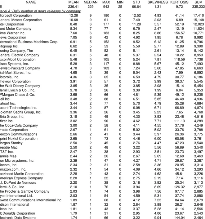
Fields like company, industry and subject deserve to be examined in detail. Table 1, Table 2 and Table 3 provide an extensive overview of what these fields precisely content. They respectively give the Factiva classification of companies, industries and topics. Nevertheless, because of the high number of companies in the sample (458), Table 1 is restricted to the 50 most important companies ranked by their sales in May 2006.

There were initially 500 different companies in the sample (all constituents of the S&P 500 in May 2006). However, only 458 out of these 500 firms will be analyzed in the subsequent GARCH and MSR econometric models, since some of these companies were created, merged, or acquired during the sample period, or present insufficient financial or news data. Figure 5 shows that news releases intensity was the highest for Microsoft (5.19% of all news releases concerned Microsoft in some way), General

Motors (4.52%), Intel (3.59%), Ford (3.53%) and Time Warner (3.21%)9. Contrary to the French market for example, the sample is quite homogeneous: we do not observe one or two firms presenting news intensity levels much above the rest of the market. Concerning industry sectors, they are split into ten general categories and 56 sub-categories. Figure 6 shows that the three sectors with the highest news frequency from May 1998 to December 2003 were Metal, Goods and Engineering (44.98%), Financial and Business Services (36.01%) and Transport and Communication (22.96%).

Subjects have also been divided into 5 general categories and 105 more specific ones, but only the general category “corporate and industrial news” is retained in our sample. From Figure 7 one can observe that the 9 most common news subjects are earnings

projections (22.44%), earnings (17.99%), ownership changes (17.51%), mergers and acquisitions (hereafter M&A, which is in fact a sub-category of ownership changes)

(16.07%), funding/capital (6.65%), capacity/facilities (4.80%), analyst

comment/recommendation (a subcategory of earnings projections) (4.33%),

contracts/orders (4.26%) and regulation/government policy (3.67%). According to Andersen (1996), we expect the impact of various news releases to be different across categories. One of the purposes of the subsequent econometric analysis will be to give some empirical support to such a theoretical prediction.

Table 4 provides an extensive set of summary statistics (mean, min, max, standard deviation, skewness, excess kurtosis and sum), for the whole sample and by company (Panel A), by industry (Panel B), by subject (Panel C) and by timing (Panel D). Note that only the 10 general categories of industries and all subcategories of topics of

corporate/industrial news (CCAT) are considered in Panels B and C. Concerning Panel D, the “timing” classification of a news release depends whether it is published when

9

Percentages do not sum up to 100%, because one news release often concerns more than one company, industry or subject. It follows that categories are not exclusive (but they are exhaustive).

the market is open (trading hours) or not (namely overnight and week-end). Daily news frequency ranges from 25 to 943 news releases a day10, with an average and a standard deviation of respectively 236.41 and 66.64. The skewness and excess kurtosis (moments of order three and four) are moderate and indicate that the total news probability distribution is asymptotically roughly Gaussian, even if it presents some substantial tails.

Panels A, B, C and D are quite interesting since they offer valuable information about possible cross-sectional differences in the news arrival rate. One of the main conclusions that can be drawn from the analysis of Table 4 is the following: the greater the total number of news releases concerning a company (or an industry, or a subject), the higher the standard deviation and the lower the skewness and kurtosis of the distribution of the daily number of news releases. Indeed, the behavior of the discrete random variable “number of news releases” is a priori best described by a Poisson probability distribution, and this distribution is known to converge to a Gaussian distribution as the number of observations increases.

4

Model specification

One of the core intermediate objectives of our work is to obtain adequate estimates of the daily stock volatility. In this aim, we choose to apply two different frameworks: GARCH(1,1) model, as used in Kalev and al. (2004), and Markov switching model that is thought to be more relevant and appropriate than the former.

10

We only consider trading days, i.e. days when the market is open. If a piece of news is released on Saturday, it will be aggregated to the news releases of the next trading day (here, if there is no holiday, Monday).

2 1 , 2 1 , 2 ,t = i + i it− + i it− i

ω

α

ε

β

σ

σ

α

β

ε

σ

ε

4.1

The GARCH model

First of all, we propose to simply replicate the study of Kalev and al. (2004) on our extensive data set. Their article aimed at testing the relation between firm-specific announcements (as a proxy for information flows) and volatility on the Australian Stock Exchange in a GARCH framework. By testing the same relation in the same framework on a richer and more extensive dataset (namely Euronext news), we want to check that we get results consistent with those of Kalev and al. (2004). However, the study we intend to perform is different from theirs in two respects: while Kalev and al. (2004) investigate the volatility behavior on an intraday and daily scale and were mainly interested in the market volatility, we choose to focus on a daily scale on the individual stock volatility.

GARCH model have now become quite common in the modeling of uncertainty in financial asset returns. We will use it as follows11:

(4-1) (4-2) where: Ri,t is the return of stock i at interval t;

Rm,t is the return of market index at interval t;

MM i

α and MM

i

β are the market model parameters for the stock i;

εi,t are the serially uncorrelated errors of stock returns i with mean zero;

and

σ

11

We use a GARCH model of order 1 since we want to rigorously replicate the study of Kalev and al. (2004). The GARCH(1,1) model is predominant in the volatility literature. Hansen and Lunde (2001) establish a forecast comparison of volatility models and conclude that “the best models do not provide a significantly better forecast than the GARCH(1,1) model”.

N

ω

α

ε

β

σ

λ

σ

=

+

+

+

The coefficients αi and βi reflect the dependence of the current volatility of stock i

upon its pasts levels and the sum α_i +β_i indicates the degree of volatility persistence.

According to Lamoureux and Lastrapes (1990) and Kalev and al. (2004)’s results, the time-varying pattern of conditional volatility may be generated by serial correlation in the information arrival process. Information clustering is indeed a well-known phenomena: news releases are not independent and are often concentrated around certain dates. In our data, the daily (resp.weekly) order-one serial correlation of our announcements is 71.09% (resp. 61.41%) and remains high for superior orders. This argument implies that when a proxy for information flows is inserted directly into the conditional variance equation, most of the observed volatility persistence is expected to disappear. Like Kalev and al. (2004), we adopt as a proxy the number of all firm-specific news events announced to the stock market per interval t (Nt), but contrary to them we run the analysis at the individual firm level (Ni,t) rather than at the market level in order to better and more precisely capture the impact of news announcements on the stock volatility. Importantly, Ni,t cannot account for the flow of private information, it does just encompass a major component of the public information set that drives stock prices and volatility. In our first analysis Ni,t is set as an exogenous variable in the conditional variance equation of the GARCH (1,1) specification as follows12:

(4-3)

Two important results follow from the estimation of the above equation. Firstly, the significance of the coefficient λi provides evidence about whether the rate of public

information arrival influences volatility of the stock i in the presence of conditional

12

Notice that variables Ni,t, Ri,t and σi,t are exactly synchronized. Ri,t is the return between the closing price

of today and the previous closing price, and Ni,t is simply the number of press releases that occurred

heteroscedasticity. Secondly, if the presence of GARCH effect is largely induced by the nature of the information flows, we may legitimately anticipate a significant decrease in the persistence of volatility, α_i +β_i . This would suggest that the positive serial correlation in the daily volatilities is partly due to the positive serial correlation in the news arrivals. Since Ni,t does not cover all sources of information, we do not expect volatility persistence to disappear entirely after the inclusion of Ni,t.

After this brief work of “replication”, we will continue our quest for an innovative explicative model of the stock volatility and develop one of the basic pieces of our work: the Markov Switching Regression.

4.2

The two-state market model (TSMM)

We propose a new way to model the stock’s variance behavior that is perfectly in line with the MDH and Roll’s (1987) results. According to Roll, the true return generating process seems to be better described by a mixture of two distributions: one corresponding to a state of information arrival, and the other to the normal return behavior. In order to study the impact of news on volatility at the firm level, our new approach is based on a combination of the well-established market model (Sharpe, 1963) and the more recent Markov Switching Regression models (MSR), largely introduced and developed by Hamilton (1989 and 1994), and significantly extended in Krolzig (1997). Our initial intuition is simple: if the occurrence of firm-specific events may have a significant impact on the variance of the firm’s return generating process, we must capture this perturbation by using a regime switching model.

In this framework, we assume that the error εi,t is state dependent. St denotes our state

2 1 2 1 = + = = + = t t if S ε Xδ Y if S ε Xδ Y

[

]

[

]

σ

ε

ε

σ

ε

ε

(mixture of two distributions with different variances) with a low-variance regime (St = 1) and a high-variance regime (St = 2):

(4-4) with Y the vector of dependent variables and X the vector of explanatory variables. The variance of the residuals for each state is given by:

(4-5)

where 2

1 2

2

σ

σ

We assume that the transition between the two regimes is governed by a Markov chain of order 1, for which the transition matrix is given by:

(4-6) where pij = p(St = i | St-1 = j) corresponds to the probability of going from state j to state

i. The unconditional probability of the regime is given by (Hamilton, 1994, p. 683):

(4-7)

The intuition underpinning our choice is simple: we anticipate that firm-specific events will impact the return variance. We will suppose that the return generating process can be adequately modeled using a two-regime process13, one regime with normal variance and one regime with high variance (firm-specific event regime). Note that, in both

13

We have realized likelihood ratio test (LR test) to compare the two-state market model (TSMM) and the classical one-state market model (MM). Since we are in the presence of nuisance parameters under the alternative hypothesis, we have implemented the procedure advocated by Davies (1977). Our results (available on request) show that the TSMM dominates the MM in all cases (i.e. for each firm) at a confidence level of 5%. Since a three-regime decomposition appears to be justified only in the presence of strong outliers, we conclude that the two-regime model is an adequate representation of the return generating process. (Note also that a two-regime model is closer to the concept of a mixture of two distributions (MDH)).

i,1 i,2 i,2 , 2 , t , 2 , , , i,1 , 1 , t , 1 , , , and ) N(0, ~ with 2 S if ) N(0, ~ with 1 S if

σ

σ

σ

ε

ε

β

α

σ

ε

ε

β

α

regimes, the MM (market model) parameters are assumed to be the same14. Therefore the return generating process is:

(4-8) where Ri,t is the return of stock i, Rm,t is the market return and St is a state variable taking

the value “1” if we are in the low variance regime and the value “2” if we are in the high variance regime. In the sequel, we will refer to equation (8) as the two-state market model (TSMM). The proposed model is a direct and parsimonious extension of the classical MM. As the regime state variable St is not directly observable, we have to specify its statistical properties. The model we propose is therefore based on the estimation of six parameters (α, β, σ1, σ2, p11 and p22) and, while much more flexible than the classical MM model, remains parsimonious.

The estimation of Markov Switching Regression models is fully presented in Hamilton (1994). It is based on a maximum likelihood approach, for which an efficient estimation algorithm has been developed. The estimated probability of being in a specific state at a specific date is one of the interesting by-products of the advocated approach. It allows one to look for the reasons explaining an increase in the variance of stock returns; in our case, to look for the link between information flow and conditional variance.

The use of this Markov Switching Regression model provides numerous interesting features. Beyond the above-quoted possibility of obtaining the estimated probability of being in a specific regime at a specific date, this specification is in line with Roll’s (1987) intuition. In his Presidential Address to the American Finance Association, he clearly highlighted that the true return-generating process seems to be better described

14

This hypothesis is supported by unreported results (available on request). We allow the market model parameters to vary across the two regimes through the estimation of a MSIAH model (Markov Switching Intercept Autoregressive Heteroscedasticity) (see Krolzig (1997)) and we find results very similar to the previous ones, except that the marginal impact of news is slightly stronger by less than one basis point.

by a mixture of two distributions, the first one corresponding to a state of information arrival and the other to the normal return behavior: it’s clearly a good candidate for testing the mixture of distribution hypothesis. Once we have estimated the probability for a firm of being in a high variance regime at a specific date, we can test whether it is linked to the information flow.

The specification has other attractive features:

- the Gaussian conditional distribution of returns could be misleading. While the model imposes a Gaussian assumption for the return distribution in each state, as shown in Hamilton (1994) and Krolzig (1997), it allows to capture skewness and kurtosis in the unconditional distribution;

- the Markov Switching Regression framework also takes conditional

heteroscedasticity into account without imposing a specific form on the conditional dependence of the variance (as in the (G)ARCH framework);

- finally, the estimation process provides us with the estimated variance in each regime, the probability of being in a specific regime at a specific date, and the estimated transition probabilities15.

- in a certain manner, the TSMM, once we have estimated the probability for a firm of being in a high variance regime at a specific date, could be a better framework than the GARCH model (via the estimated

λ

the impact of the public information rate on the stock volatility at the individual firm level. This may also give some additional robustness to the news-volatility relation in the pattern of the daily stock return volatility.

15

All estimations presented in this paper have been realized under the Ox econometric software, using the Krolzig MSVAR package. We thank Professor J. Hamilton for advising the use of this package. It is freely downloadable at: http://www.nuff.ox.ac.uk/Users/Doornik/index.html.

5

The results

5.1

GARCH framework

We begin with the GARCH specification. In a first step, we merely reproduce the methodology commonly used in the literature (see Kalev et al. (2004) and Janssen (2004)). It sums up to insert the number of daily announcements concerning a stock into the equation of its variance in a GARCH (1,1) model. The estimation of the latter after inclusion of the variable NBN (daily number of news releases) converges for 445 stocks. Out of those 445 estimations, the coefficient associated to the NBN variable is significant at the 5% (resp. 10%) level in 161 (resp. 212) cases and its inclusion decreases the persistence (alpha + beta) in 403 cases. It is important to notice that the estimation of a GARCH on such a long period may not be without problems. Therefore, results are probably not totally exempt of methodological biases. Beyond this reserve, it gives a first insight of how the information stream affects the conditional volatility and to which extent it can explain the well-known persistence of the latter. It is unfeasible to give extensively here the results for each of the 458 companies of the sample, but they are available upon request.

5.2

MSR framework: the two-state market model (TSMM).

5.2.1

Panel data analysis with the smooth probability

5.2.1.1

Global analysis

For the many reasons brought up in Section 2.1, an MSR framework is expected to be a more appropriate specification and to fit much better than a GARCH model. As it was thoroughly explained in the same section, such an approach leads us to develop a two-state market model that provides us with the (daily) probabilities of being in a high

volatility regime on a specific day for each stock of the sample. Once these probabilities have been obtained, it is possible to regress them over our explicative and control variables, in a panel framework.

The main advantage of the panel analysis is to work globally and to analyze the combination of time and cross-sectional effects. Modeling in this setting calls for some complex stochastic specification. We therefore use the most common techniques: the fixed effects and random effects approaches.

The fixed effects approach takes the constant model to be a group-specific term in the regression model. The constant is different for any security. It should be noted that the term “fixed” as used here indicates that the constant term does not vary over time. The random effects approach assumes that the residual is a group specific random element. In this model, the constant is the same for all securities included in the sample. The crucial distinction between these two cases is whether the unobserved individual effect embodies elements that are correlated with the regressors in the model, not whether this effect is stochastic or not. In our case, the fixed effects model is probably better specified. Indeed, from the relatively high heterogeneity across stocks observed in the individual regressions, we may think that the fixed effects approach fits better, since it assumes the constant to be different for each stock. Moreover, from a statistical perspective, Hausman’s test (available on request) indicates that the fixed effects model performs much better than the random effects one.

As a regression method, we opt for a General Method of Moments (GMM) regression16 rather than a classical OLS regression because we expect the residuals of our regression

16

Before adopting the GMM framework, we first used an « improved » OLS approach like « weighted least squares »: results are very similar to those obtained by GMM, and even more significant. However, we think that a GMM regression must be preferred to an (even improved) OLS regression since the former is known to be much more robust than the latter to heteroscedasticity and serial correlation problems apparent in our data. Moreover, GMM coefficients are directly interpretable as such, whereas

t i t i t i t i C C Prob, = + +β′x, +ε ,

to present substantial heteroscedasticity and serial correlation problems. The coefficients obtained by this approach are the same as the coefficients delivered by the classical OLS regression, but the GMM procedure provides Student statistics robust to heteroscedasticity and serial correlation of order one. The estimate of the covariance matrix is obtained thanks to the convergent estimator of Newey and West (1987).

We conduct thus the following fixed-effect panel GMM regression in order to measure the impact of the announcements arrivals on the probability to be in the high volatility regime (the “smooth” probability):

(5-1) where Prob_i,t stands for the probability of stock i at time t to be in the high volatility

regime and x_i,t the variables for which we anticipate some kind of association with

t i

Prob_, . The heterogeneity, i.e. the cross-sectional effect between stocks, is modeled by

i

C where Ci is a constant term specific to individuals. We also add a time effect, Ct, in

order to take into account the possible evolution of the intercept through time. Specifically, we code this variable C_t as four annual dummies.

The use of a probability as a dependent variable mainly raises an issue of heteroscedasticity (see Greene (2002)). We solve it by using the Newey-West robust estimator of the covariance matrix.

In our first specification, our proxy for the information flow is a dummy equal to one if there is at least one news release concerning stock i in t and 0 otherwise. The control variables which are not accounted for by the fixed effect, because they are not constant on the selected period, are the conditional volatility of the market and of the sector index (the latter is formed on the basis of the two first digits of the SIC code). Both

“weighted least squares” coefficients are not, since the variables have been logit-transformed because they are proportions.

t i t i t t i i t i C D varmrkt varsect Prob, = +β1 , +β2 +β3 , +ε ,

conditional variances of the market portfolio and of the sector index are estimated via a GARCH (1,1) model.

(5-2)

It follows from Table 5 that after controlling for annual, fixed, market and sectorial effects, the fact to be on a date where at least one Reuters news release has been recorded for a stock increases the probability to be in the high variance regime of about 6.75 points for this stock. Not surprisingly, the coefficients of the market and sector variances appear to be positive and significant, since the stock volatility is known to convey some market component. Such control variables allows us to account (at least partially) for all macroeconomic shocks that affect the stock volatility and that are not covered by our set of firm-specific press releases.

It also appears (from results available on request) that the annual dummies denoted by

Ct are systematically significant when they are introduced, which seems to suggest that

the probability to be in the high variance regime exhibits some pattern through time and cannot be taken as independent of time. Therefore, we will perform our regressions of Section 5.2.1.3 (except in Table 10 in order to be able to compare US results to the French ones) by systematically including this variable Ct in order to control for the time pattern of the probability of being in the high variance regime.

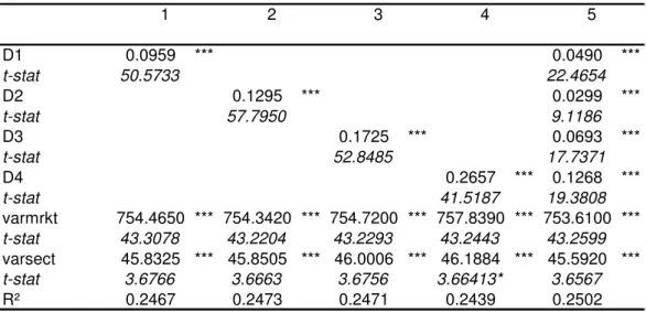
As a next step we wish to measure the impact of the information volume on this latter probability. Our idea is to introduce four dummies Dk,i,t (k=1, …, 4) in order to split the trading days in different categories according to the level of communication observed everyday: D1,i,t (resp. D2,i,t, D3,i,t, D4,i,t) = 1 if the trading day t is in the top 20% (resp. 10%, 5%, 1%) of the days presenting the highest number of news releases concerning stock i, and 0 otherwise.

t i t i t t i k i t i C D varmrkt varsect Prob, = +β1 ,, +β2 +β3 , +ε , t i t i t t i t i i t i C NBN NBN varmrkt varsect Prob_, = +β_{1 ,} +β₂ 2_, +β₃ +β_{4 ,} +ε _, (5-3)

Results of Table 6 show clearly that the probability to be in the high variance regime increases with the volume of announcements: a trading day situated in the top 1% of the most “news-intensive” trading days brings 26.6 extra points to the variance of the concerned stock, which cannot be considered as negligible, both from a statistical and economical points of view.

This new evidence leads us to propose a specification including directly the number of announcements in the regression equation:

(5-4)

t i

NBN_, is the total number of announcements observed for stock i on day t while

2 ,t i

NBN is simply the square of NBN_i,t. This last variable is introduced in order to take

into account the possibility of a marginally decreasing (or increasing) effect of the number of news releases on the probability of high variance regime.

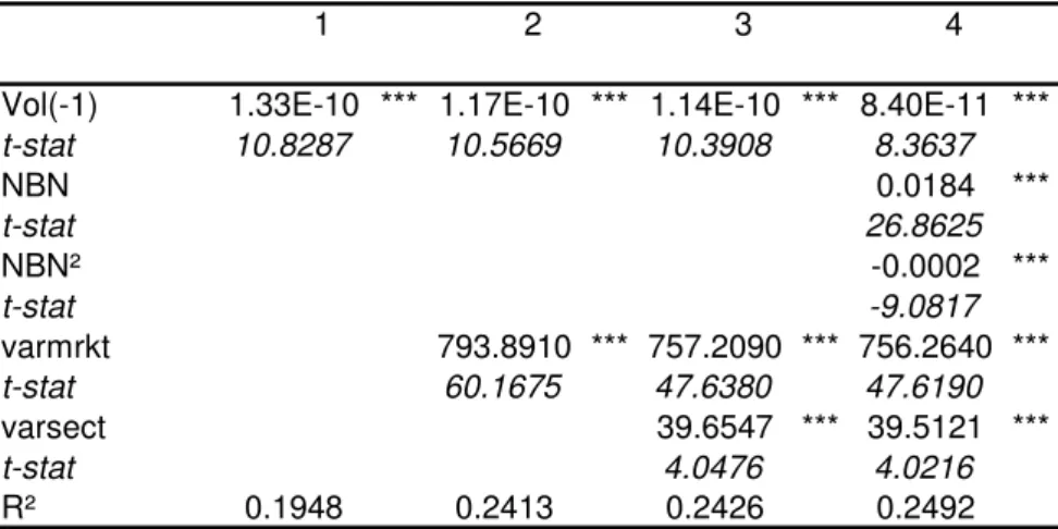
Results of Table 7 demonstrate the positive and significant impact of the volume of specific announcements on the conditional volatility of each stock. The significant negative sign associated to NBN² suggests the existence of a marginally decreasing effect, with maximum situated around 64.5 news releases.

In line with Kalev et al. (2002), p. 1444, we introduce the trading volume in value ($) into the regression equation, “as this variable does, to a limited degree, contain private information not yet reflected in public news. It could also influence volatility in ways that are unrelated to the information arrival”. Indeed, our variable NBN, because it is of public knowledge, does not take into account the private dimension of information. In order to avoid any endogeneity problem, we lag this volume variable by one period:

t i t i t t i t i t i i t

i C NBN NBN Vol varmrkt varsect

Prob_, = +β_{1 ,} +β₂ 2_, +β_{3 ,}−₁+β₄ +β_{5 ,} +ε _, t i t i t t i t i D NBN varmrkt varsect NBN D2002 , 7 2003 , 8 9 , , 6 β β β ε β ⋅ ⋅ + ⋅ ⋅ + + + + (5-5)

According to Table 8, the impact of trading volume on the probability of high variance regime turns out to be positive and significant, which is a well-known result of the literature. We refer the interested reader to Karpoff (1987) for a detailed survey of earlier empirical work, most of which shows evidence that higher volatility is accompanied by higher trading volume. More recent studies such as Jain and Joh (1988), Schwert (1989), Gallant et al. (1992), Richardson and Smith (1994), Foster and Viswanathan (1995), and Andersen (1996) also document a similar relation. Notice that this impact of the volume trading remains significant after the inclusion of our public information proxy (NBN).

5.2.1.2

Introduction of a time effect

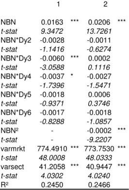
Up to now, we have not considered the possibility that the impact of the announcements frequency on the smooth probability could vary through time. We therefore propose to perform the following panel regression:

t i Prob_, t i t i t i t i t i t i C NBN NBN D NBN D NBN D NBN C + + _{1 ,} + ₂ 2_, + ₃⋅ ₁₉₉₉⋅ _, + ₄ ⋅ ₂₀₀₀⋅ _, + ₅⋅ ₂₀₀₁⋅ _, =

β

β

β

β

β

Ct takes into account as before the possible evolution of the intercept through time,

while the coefficients

β

β

Results of Table 9 show that the link between this probability and our explicative variable does not seem to depend on time. It provides thus some evidence in favor of the stability of the relation between the news flow and the volatility.

5.2.1.3

Analysis by category

5.2.1.3.1

Categorization by topic

Public information is not homogeneous. We must consider the possibility that a news release about merger and acquisition does not affect the stock volatility the same way as an earnings announcement for example. Similarly, information released during trading hours may not have the same impact on the stock volatility as information released during non-trading hours. From a theoretical perspective (see Andersen (1996)), the topic and the timing of each news release matter. We check this point by running the same regression as above on a limited category of news releases. We first retain the seven most common subject categories, that we also used on the French market: Merger and Acquisition (M&A) (Factiva code C181), Earnings (C151), Earnings Projections (C152), Analyst Comments and Recommendations (C1521) which is a subset of the latter, Funding/Capital (C17), Regulation and Government Policy (C13) and, finally,

Contracts/Orders (C33). We also add two more categories that did not appear in our French study: Ownership Changes (C18), which is a little more general than M&A, and in particular Earnings Surprises (C1514), which contained a too weak number of observations to be considered in the French study.

Results for the US market are synthesized in Table 10 and results from our previous study on the French market are reproduced in Table 11 for the sake of comparison. If the regressions are run individually for each category, with the conditional market and sector variances as the usual control variables, all coefficients (for NBN) obtained with

our US data are significant at the 1%-level and are very similar to the ones obtained on the French market.

If we forget about the “Earning surprises” categories for a while, the

Regulation/Government Policy news is still the kind of announcement with the highest

impact on the stock conditional volatility, followed by the Analyst

Comment/Recommendation category. Other categories present coefficients similar on the French and US market, with some only slight variations.

A particular emphasis must put on a newly introduced topic: “Earnings surprises”. The coefficient is impressive: one earning surprise increases (on average) the probability of being in a high volatility regime by about 24 points (=coefficient of NB + coefficient of

NB²). It seems that this kind of news release increases significantly the uncertainty of investors about future prospects of the firm.

We give now the results for three subjects in particular: Regulation / Government Policy

(C13) (Table 12), Ownership Change (C18) (Table 13) and Contracts (C33) (Table 14), and we subdivide these latter general categories into more accurate ones to investigate what kind of news brings more or less volatility to the stock return. Notice also that we now introduce temporal dummies (but we do not report their coefficients) to take into account of a possible time pattern of the conditional volatility.

The more detailed subdivision that we apply here delivers a very interesting fact: the coefficient of the category C183Privatization is significantly negative (-0.0622). If we compare it to the coefficient of C131Regulatory Bodies, which is in contrast the highest one, with 0.1498, we have two extreme types of topics and of effects. While privatization news seems to calm down the investors and to decrease the uncertainty around the stock value, news from the regulator affects the volatility in a completely different way and tends to increase the uncertainty around the prospects of the company.

i i i

i C NBN MV

ProbTrans = +βln( )+δln( )+ε

The fact that investors resent the intervention of the State as more unsafe than the intervention of private investors or companies is maybe not so unexpected, but tells a lot about the current prejudices and judgments of the market…

5.2.1.3.2

Categorization by timing

As in the French case, we can make a distinction between the announcements arriving when the market is open or closed. We thus define two timing categories: news released during Trading Hours and news released during Non-Trading Hours (mainly week-end and overnight). Results are qualitatively similar to the ones obtained on the French market. An announcement occurring during a trading day seems to bring more uncertainty than another arriving during the WE or overnight for example.

5.2.2

Cross-sectional data analysis with the transition probability

A nice characteristic of the MS-var estimation is to offer us the possibility to obtain the transition probabilities from one state (here, one variance regime) to another. Notice that those transition probabilities are not available on a daily basis as the previous smooth probabilities, but only in the cross-sectional dimension. It follows that we have got two transition probabilities (from the high regime to the low one, and vice-versa) for each firm. As a next step in our analysis, we can try to explain these probabilities by some characteristics specific to the firm. Our first attempt is to investigate the link between those transition probabilities and the level of communication prevailing around a given firm. We choose as a first proxy of the latter the log of the daily average number of announcements ln(NBNi) (which is supposed to measure the intensity of the flow of

information for a given stock):

t t t C Rhô NBN

NBN = + ⋅ −1 +ε

where ln(MV_i) is the average market value of the firm on the sample period. We use it as a control variable, because the number of news releases is logically higher for large firms than for smaller ones.

As a second proxy, we choose NBDays-NBN: the percentage of trading days where at least one announcement was observed (which is supposed to measure the regularity of the information flow).

In order to estimate the persistence of the communication of each company, we specify and perform an AR(1) individually for each firm and regress the number of news releases in t on the number of news releases on the previous day t-1:

(5-8) ln(Rhô), our third proxy, measures the persistence of the communication: if ln(Rhô) is high, it implies that a day with a high number of news releases is likely to be followed by another day with a high number of announcements as well.

Table 16 presents results of univariate and multivariate regressions. Notice that the coefficient of the log proxies must be interpreted as elasticities, or semi-elasticities. For example, we deduce from the coefficients of ln(NBN_i) that if a stock has a daily average number of announcements NBN_i 10% higher than another stock, its probability of transition from the high to the low (resp. from the low to the high) variance regime is about 13 (resp. 58) basis points higher. Our proxies of communication characteristics seem to have a higher impact on the probability of transition from the low variance regime to the high variance regime, and thus a stronger effect on the probability to present a more volatile behaviour of stock returns. This seems consistent with our previous results: if the probability of transition L-H increases more than the probability of transition H-L when there are a lot of announcements, it is logical that the probability

of being in the high variance regime is higher as well. The higher and the more regular the communication intensity of a firm, and the faster the volatility of its stock will arrive in the high regime. However, once the volatility is in the high regime, a firm communicating a lot can expect to come back quicker to the low volatility regime than a firm which does not.

Our interpretation must nevertheless remain cautious. We cannot exclude the presence of an endogeneity problem, since the sense of the causation is not straightforward: does a higher communication trigger a change of regime, or, the other way around, does a change of regime that triggers a higher communication about the company? The current results leave the issue open, and we consider the latter as a potentially nice track for future research.

The interested reader will find descriptive statistics about the main variables used in this section in the Appendix.

6

Conclusion

Without a shadow of a doubt, research works aiming at accurately identifying and understanding the link between information diffusion and stock prices are of prime importance and interest, as much for the academic world as for business corporations. In this general context, the main objective of our study is to investigate the impact of the news arrivals intensity on the stock price volatility. We use daily prices and Reuters (and Dow Jones as well) news releases concerning all stocks pertaining to the S&P 500 index over the period ranging from May 13, 1998 to December 31, 2003. We first begin with a partial replication of the Kalev and al. (2004)’s GARCH model and we find, like them, and identically to our previous French study on the topic, that public information explains a large part of the daily volatility persistence. We apply a Markov switching

regression (MSR) model to the data in order to determine the daily probability of the volatility regime to be in a high level state or a low level state. Our developed MSR model presents many interesting features: its structure is more general than the GARCH models’ one, they more often converge towards a stable solution and they implicitly rest on a theoretical argument: the Mixture of Distribution Hypothesis. We find for each stock a positive and (5%-)significant relation between the daily number of news and the daily probability of being in a high volatility state. The panel analysis confirms these results since the above detected positive relation remains highly significant, even when controlling for the volume of trades and the conditional sector and market variances A positive and significant relation between news arrivals intensity and stock prices volatility seems thus to be reasonable and consistent. Hence it follows that news contains some relevant and valuable i