Accepted Manuscript
A fuzzy expected value approach under generalized data envelopment analysis Mohammadreza Ghasemi, Joshua Ignatius, Sebastián Lozano, Ali
Emrouznejad, Adel Hatami-Marbini
PII: S0950-7051(15)00243-9
DOI: http://dx.doi.org/10.1016/j.knosys.2015.06.025
Reference: KNOSYS 3200
To appear in: Knowledge-Based Systems
Received Date: 20 January 2015
Revised Date: 2 June 2015
Accepted Date: 18 June 2015
Please cite this article as: M. Ghasemi, J. Ignatius, S. Lozano, A. Emrouznejad, A. Hatami-Marbini, A fuzzy expected value approach under generalized data envelopment analysis, Knowledge-Based Systems (2015), doi: http:// dx.doi.org/10.1016/j.knosys.2015.06.025
This is a PDF file of an unedited manuscript that has been accepted for publication. As a service to our customers we are providing this early version of the manuscript. The manuscript will undergo copyediting, typesetting, and review of the resulting proof before it is published in its final form. Please note that during the production process errors may be discovered which could affect the content, and all legal disclaimers that apply to the journal pertain.
© 2015, Elsevier. Licensed under the Creative Commons Attribution-NonCommercial-NoDerivatives 4.0 International
A fuzzy expected value approach under generalized data
envelopment analysis
Mohammadreza Ghasemi
School of Mathematical Sciences
Universiti Sains Malaysia
11800 Minden
Penang, Malaysia
Email: [email protected]
Joshua Ignatius
1School of Mathematical Sciences
Universiti Sains Malaysia
11800 Minden
Penang, Malaysia
Tel: +604-6533384
Fax: +604-6570910
Email:[email protected]
Sebastián Lozano
Department of Industrial Management,
University of Seville, Spain
E-mail: [email protected]
Ali Emrouznejad
Aston Business School
Aston University
Brimingham, UK
Email: [email protected]
Adel Hatami-Marbini
Louvain School of Management
Center of Operations Research and Econometrics (CORE)
Université catholique de Louvain,
34 voie du roman pays, L1.03.01 B-1348 Louvain-la-Neuve, Belgium
E-mail: [email protected]
A fuzzy expected value approach under generalized data
envelopment analysis
A B S T R A C T
Fuzzy data envelopment analysis (DEA) models emerge as another class of DEA models to account for imprecise inputs and outputs for decision making units (DMUs). Although several approaches for solving fuzzy DEA models have been developed, there are some drawbacks, ranging from the inability to provide satisfactory discrimination power to simplistic numerical examples that handles only triangular fuzzy numbers or symmetrical fuzzy numbers. To address these drawbacks, this paper proposes using the concept of expected value in generalized DEA (GDEA) model. This allows the unification of three models – fuzzy expected CCR, fuzzy expected BCC, and fuzzy expected FDH models – and the ability of these models to handle both symmetrical and asymmetrical fuzzy numbers. We also explored the role of fuzzy GDEA model as a ranking method and compared it to existing super-efficiency evaluation models. Our proposed model is always feasible, while infeasibility problems remain in certain cases under existing super-efficiency models. In order to illustrate the performance of the proposed method, it is first tested using two established numerical examples and compared with the results obtained from alternative methods. A third example on energy dependency among 23 European Union (EU) member countries is further used to validate and describe the efficacy of our approach under asymmetric fuzzy numbers.
Keywords: Data envelopment analysis; Generalized data envelopment analysis; Fuzzy expected value; Super-efficiency; Symmetric & asymmetric fuzzy numbers
1. Introduction
Data envelopment analysis (DEA) was first proposed by Charnes, Cooper, & Rhodes (1978) and later become known as the CCR model. BCC model (Banker, Charnes, & Cooper, 1984) extends the CCR model by accommodating for variable returns to scale. Concurrently, the Free Disposal Hull (FDH) model (Deprins, Simar, & Tulkens, 1984) was developed as an alternative DEA model which benefits from a mixed integer programming to calculate the relative efficiencies of decision making units (DMUs). In order to treat basic CCR, BCC and FDH models in a unified way, a generalized DEA model (GDEA) was proposed by Yun, Nakayama, & Tanino (2004). Since traditional DEA models do not account for subjective input and output values, another class of DEA models emerged; that is, fuzzy DEA models (Emrouznejad & Tavana, 2014; Hatami-Marbini, Emrouznejad, & Tavana, 2011a).
Several solution approaches have been developed for fuzzy DEA models, which include: 1) the defuzzification approach (Ghasemi, Ignatius, & Davoodi, 2014a; Hasuike, 2011; Wang & Chin, 2011), 2) the α-level based approach (Azadeh, Moghaddam, Asadzadeh, & Negahban, 2011; Azadeh, Sheikhalishahi, & Asadzadeh, 2011; Muren, Ma, & Cui, 2012; Puri & Yadav, 2012; Zerafat Angiz L, Emrouznejad, & Mustafa, 2010), 3) fuzzy ranking (Bagherzadeh valami, 2009; Guo & Tanaka, 2001; Hatami-Marbini, Saati, & Tavana, 2011b; Hatami-Marbini, Tavana, & Ebrahimi, 2011c; Soleimani-damaneh, 2009), 4) the possibility approach (Khodabakhshi, Gholami, & Kheirollahi, 2010; Lertworasirikul, Fang, Joines, & Nuttle, 2003), 5) fuzzy arithmetic (Wang, Greatbanks, & Yang, 2005; Wang, Luo, & Liang, 2009), and 6) the fuzzy random/type-2 fuzzy set (Qin & Liu, 2010; Qin,
Liu, & Liu, 2011; Qin, Liu, Liu, & Wang, 2009). Fuzzy ranking and α-cut approaches are the most popular as outlined in a survey on fuzzy DEA literature (Hatami-Marbini et al., 2011a). However, existing fuzzy DEA models exhibit some drawbacks.
The first major drawback of existing fuzzy DEA in the literature is the significant computational effort in solving the efficiency values. Guo and Tanaka’s fuzzy ranking approach (Guo & Tanaka, 2001) needs two linear programming problems to obtain the efficiency value for any givenDMU. The process involves feeding the optimal solution of the primary linear programming problem as coefficients of some fuzzy constraints into the second linear programming problem. The same computational complexity is also inherent in the fuzzy possibilitic approach proposed by Lertworasirikul et al. (2003), where fuzzy constraints and objective function are defined across different possibility levels or α-cut. In the case ofn DMUs and five levels of possibility, there are 5n+2
linear programming problems to be solved, which remains computationally expensive. This problem also arises in α-level based approaches; it requires solving a sequence of linear programming models, thus leading to an increase in computational effort for obtaining fuzzy efficiencies of DMUs. Since there are different optimal solutions for each α-level, the decision maker (DM) is left to decide on which solution is the best for the scenario under his or her interpretation. In most cases, the decision analyst would decide based on the number of efficiencies that are generated across all α-cuts before deciding on the final ranking solution.
The second limitation in existing fuzzy DEA models is the focus on triangular fuzzy membership functions (see León, Liern, Ruiz, & Sirvent, 2003) or symmetrical triangular fuzzy membership functions (see Guo & Tanaka, 2001). There is much left unexplored for inputs and outputs that are imprecise and do not conform to the said fuzzy membership functions.
The third drawback in existing fuzzy DEA models is its limited scope and much emphasis placed on the CCR model (see Wang & Chin, 2011). The unification of CCR, BCC and FDH comes under the category of GDEA model. Considering imprecision, Jahanshahloo, Hosseinzadeh-Lotfi, Malkhalifeh, & Ahadzadeh-Namin (2009) are among the first authors to formulate the GDEA model with interval data (IGDEA); such that the upper bound efficiency value is obtained considering that the DM is optimistic for theDMU under evaluation (DMUo), while pessimistic with the
remainingDMUs in the evaluation set. Contrastingly, the lower bound efficiency values is obtained by considering that the DM is pessimistic for theDMU under evaluation (DMUo), while optimistic
with the remainingDMUs in the evaluation set. This is achieved by selecting only the extreme points in an interval for the input and output measures. It does not derive information using the form of a particular function, such as one expressed in fuzzy or possibilitic manner. In other words, the mid-values as appear in a fuzzy numbered dataset are effectively ignored and the results of efficiency covers a range comprising of an interval made up off overly optimistic and pessimistic in the
computational effort than competing models. We further propose a ranking method for efficient DMUs by adapting the FEGDEA and illustrate that our approach does not suffer from infeasibility issues as may be the case for existing methods.
In order to tackle the existing drawbacks in the fuzzy DEA literature, we propose the use of expected value approach for unifying all three models – fuzzy CCR, fuzzy BCC and fuzzy FDH models. In particular, our research process entails the following objectives. First, we investigate the performance of our method with existing method that handles symmetrical data. Second, we show that integrating the fuzzy expected value approach into the GDEA model outperforms integrating the fuzzy expected value in classical DEA models. Third, when efficient cases are to be ranked such as in super-efficiency analysis, the use of Andersen and Petersen (1993) approach in FEGDEA model removes the issue of infeasibility, which occurs when it is applied to classical DEA models in certain cases. Fourth, we further show that having addressed all the above objectives, our proposed model is able to generate results under the CCR, BCC and FDH forms including ranking efficient units for both symmetrical and asymmetrical data.
The rest of the paper is structured as follows. Section 2 provides the preliminaries on the pertinent mathematical concepts on fuzzy DEA. Section 3 gives a brief description of the basic DEA models and GDEA model. Section 4 outlines the development of the proposed model. Section 5 illustrates a ranking method for the proposed model and suggests ways to discriminate those efficient DMUs. Section 6 describes the proposed method with two established numerical examples and a third example on an energy dependency case among 23 European Union (EU) member countries. The performance of our proposed model is compared to other existing methods for performance validation. Section 7 concludes the study.
2. Preliminary concepts
Definition 1. IfX is a collection of objects denoted byx, called the universe, then a fuzzy set A% inX is a set of ordered pairs:
(
)
{
, A}
A%= x m% xÎX ,
in which mA%( )x is called the membership function ofx in A% that ( ) :
[ ]
0,1A x X
m% ® .
Definition 2.The α-level (or α-cut) set of a fuzzy set A% is a crisp subset ofX and is denoted by:
{
}
( ) A( )
Aa = xÎX m% x ³a .
Definition 3.A fuzzy set A% of setX is convex if
(
)
(
1 1 2)
min{
( ),1 ( ) ,1}
A x x A x A x
Definition 4.A fuzzy number A% is a convex normalized fuzzy set A% of real line ¡, in which there exists at least one xoΡ, with mA%(xo)=1 and mA%( )x is piecewise continuous. A fuzzy number
(
l, m1, m2, u)
A%= a a a a is a trapezoidal fuzzy number if
1 1 1 2 2 2 , , 1, , ( ) , , 0, . l m l m l m m A u m u m u x a a x a a a a x a x a x a x a a a otherwise m ì - £ < ï -ï ï £ £ ï = í -ï < £ ï -ï ïî %
The α-level set of the trapezoidal fuzzy number A% can be denoted as an interval, éëfl( ),a fu( )a ùû, in which fl( )a =al +a(am1 -al) and fu( )a =au -a(au -am2) where aÎ
[ ]
0,1 .Remark 1. By assuming am =am1 =am2 in a trapezoidal fuzzy number A% =
(
a al, m1,am2,au)
weobtain a triangular fuzzy number as A%¢ =
(
a al, m,au)
. If we assume am1 -al =au -am2 in thetrapezoidal fuzzy number A% and am-al =au-am in the triangular fuzzy number A%¢ we have symmetrical trapezoidal and triangular fuzzy numbers, respectively.
Definition 5 (Heilpern, 1992). The expected interval (EI) and the expected value (EV) of a fuzzy number A% are defined as follows:
( )
1 1 1 , 2 0 ( ) , 0 ( ) A A l u EI A =ëéE E û êù=é f a ad f a ad ùú ëò
ò
û % ;( )
1 2 2 A A E E EV A% = + . If we assume that A%=(
a al, m1,am2,au)
is a trapezoidal fuzzy number then( )
1 2 , 2 2 m m l u a a a a EI A = êé + + ùú ë û % ;( )
1 2 4 m m l u a a a a EV A% = + + + .If we further assume that is a triangular fuzzy number then
( )
, 2 2 l m m u a a a a EI A = êé + + ùú ë û % ;( )
2 4 l m u a a a EV A% = + + . 3. BackgroundConsider we are interested in evaluating the relative efficiency of n DMUs which use m inputs to produce s outputs. The m-input-s-output data can be expressed as xij
(
i=1,..., ,m j=1,...,n)
and(
1,..., , 1,...,)
rj
3.1. Basic DEA models
The envelopment form and dual (multiplier) form of input-oriented BCC model can be formulated in a linear programming framework as follows (Cooper, Seiford, & Tone, 2007):
The envelopment form of BCC model: The dual (multiplier) form of BCC model:
o minq 1 s o r ro o r maxq u y c = =
å
-s.t. 1 , 1,..., , n j ij o io j x x i m l q = £ =å
s.t. 1 1, m i io i v x = =å
1 , 1,..., , n j rj ro j y y r s l = ³ =å
(1) 1 1 0, 1,..., , s m r rj i ij o r i u y v x c j n = = - - £ =å
å
(2) 1 1, n j j l = =å
ur ³0, r=1,..., ,s 0, 1,..., , i v ³ i= m 0, 1,..., , j j n l ³ = co free in sign,whereλ1, …,λnare non-negative variables in model (1), andur(r = 1,…, s) andvi(i = 1,…, m) are the
input and output weights assigned to input i and output r, respectively in model (2). The input-oriented CCR model can be easily obtained by removing the condition
å
jlj =1 in model (1) and by assumingco= 0 in model (2). FDH model is derived when condition ljÎ{ }
0,1 is added to the BCCmodel (1).
Definition 6(Cooper et al., 2007). DMUois efficient if the optimal value of the objective function (qo*
) is equal to 1, and is considered inefficient if qo*<1. However,DMUo is fully (or Pareto-Koopmans)
efficient if qo*=1 and there exists at least one optimal solution (u*,v*), withu*> 0 &v*> 0, where *
o
q
and (u*, v*) are the optimal value of the objective function and values with non-negative constraints
given in model (1), respectively. By considering model (2), the values of the input excesses (si-) and the outputs shortfalls (sr+) for anyi &r can be defined as follows:
( )
1 n i o io j ij j s- q x l x i = = -å
" &( )
1 n r j rj ro j s+ l y y r = =å
- " ,where si-(i= 1,…,m) and sr+ (r = 1,…,s) are identified as slack variables for any feasible solution (θ,λ) of model (1). ThenDMUo is fully (or Pareto-Koopmans) efficient if qo*=1 and all optimal slack
values are zero.
All efficient DMUs register efficiency values of 1. In order to discriminate between efficient DMUs, Andersen & Petersen (1993) proposed the super efficiency method. The technique enables an extreme efficientDMUo to achieve an efficiency value greater than one by excluding theDMUo from
the reference set in the DEA model.
o minq s.t. 1, , 1,..., , n j ij o io j o x x i m l q = ¹ £ =
å
1, , 1,..., , n j rj ro j o y y r s l = ¹ ³ =å
(3) 1, 1, n j j o l = ¹ =å
0, 1,..., , j j n l ³ =3.2. Generalized DEA (GDEA) model
The GDEA model proposed by Yun et al. (2004) unifies the CCR, BCC, and FDH models, which can be formulated as follows: maxD s.t.
(
)
(
)
1 1 , 1,..., , s m j r ro rj i io ij r i d a u y y v x x j n = = é ù D £ + ê - - - + ú = ëå
å
û 1 1 1, s m r i r i u v = = - =å
å
0, 0, 1,..., , 1,..., , r i u ³ v ³ i= m r= s (4)where a >0 is the user-specified value and appropriately given according to the specified problems
(see definition 6) and
{
(
) (
)
}
,
max ,
j r ro rj i io ij
i r
d = u y -y v -x +x and the optimal value of objective function ( *) are always non-positive.
Definition 7 (Yun et al., 2004). For a given positive α value, DMUo is said to be α-efficient if and
only if the optimal value of GDEA model (4) is equal to zero, otherwise it is defined as α-inefficient. It was also proved by Yun et al. (2004) that
(i)DMUo is FDH-efficient ifDMUo is α-efficient for some sufficiently small positive value of α.
(ii)DMUo is BCC-efficient ifDMUo is α-efficient for some sufficiently large positive value of α.
(iii) DMUo is CCR-efficient if DMUo is α-efficient for some sufficiently large positive value of α
when the condition,
1 1 0 s m r ro i io r i u y v x = = - =
å
å
, is added to model (4).4. Fuzzy GDEA Model Using Fuzzy Expected Value
Suppose there aren DMUs to be evaluated, which use m inputs to produce s outputs. According to definition 4, assume that data of inputs and outputs are uncertain and can be expressed by fuzzy trapezoidal numbers with bounded support
(
l, m1, m2, u)
ij ij ij ij ij
x% = x x x x , i = 1,…,m, j = 1,…,n,
(
l , m1, m2, u)
rj rj rj rj rj
We use the GDEA model (4) to evaluate the relative efficiencies of a set of DMUs. The GDEA model can be transformed into the following LP form of the fuzzy expected value model.
maxD s.t. ( ) 1
(
)
1(
)
, 1,..., , s m j r ro rj i io ij r i E d aE u y y v x x j n = = æ ö D £ + ç - - - + ÷ = èå
å
ø % % % % % 1 1 1, s m r i r i u v = = - =å
å
0, 0, 1,..., , 1,..., , r i u ³ v ³ i= m r= s (5)where a >0 is defined as in the model (4) and
{
(
(
)
)
(
(
)
)
}
,
max ,
j r ro rj i io ij
i r
d% = E u y% -y% E v -x% +x% . In GDEA model (4), for any given positive α value, we use the optimal value of the objective function to estimate whether DMUo is α-efficient or α-inefficient. Similarly, in the proposed model
(5), the value of α is applied to characterizeDMUo as α-efficient or α-inefficient. If * = 0, we consider
DMUo as α-expected-efficient; otherwise, it is mentioned as α-expected-inefficient.
The above fuzzy expected LP problem is able to transform into its crisp equivalent form. Let us continue by considering the following proposition:
Proposition 1(Liu & Liu, 2003).Letλ andγ be fuzzy numbers. Then for any non-negative numbersa andb, we have
(
)
( )
( )
E al+bg =aE l +bE g .
According to definition 5 and proposition 1, the FEGDEA model (5) can be transformed as follows: maxD s.t.
(
1 2 1 2)
1 1 4 s m m m m l u l u j r ro ro ro ro ro rj rj rj r d a u y y y y y y y y = ì D £ + í + + + - - - -îå
%(
1 2 1 2)
1 1 , 1,..., , 4 m m m m m l u l u i io io io io ij ij ij ij i v x x x x x x x x j n = ü - - - + + + + ý = þå
1 1 1, s m r i r i u v = = - =å
å
0, 0, 1,..., , 1,..., , r i u ³ v ³ i= m r= s (6)wherea >0 is appropriately assigned to the problem and
(
1 2 1 2)
, max , 4 m m m m l u l u r j ro ro ro ro ro rj rj rj i r u d = ìí y +y +y +y -y -y -y -y î %(
1 2 1 2)
4 m m m m l u l u i io io io io ij ij ij ij v x x x x x x x x ü - - - - + + + + ý þ.Definition 8. Similar to the GDEA model (4), the above model (6) exhibits the following properties: (i)DMUo is fuzzy FDH-expected-efficient ifDMUois
α
-efficient for some sufficiently small positivevalue of α.
(i)DMUo is fuzzy BCC-expected-efficient ifDMUo is α-efficient for some sufficiently large positive
(ii)DMUo is fuzzy CCR-expected-efficient ifDMUo is α-efficient for some sufficiently large positive
value of αwhen the following conditionis added to model (6).
(
1 2)
(
1 2)
1 1 0 s m m m m m l u l u r ro ro ro ro i io io io io r i u y y y y v x x x x = = + + + - + + + =å
å
.In the same manner, the basic DEA models (1) and (2) can be adapted to the fuzzy expected LP form. This means that the fuzzy expected LP form can be transformed into its crisp equivalent, while preserving the fuzzy values. Interested readers are referred to Wang and Chin’s method (Wang & Chin, 2011). Hence, the BCC-DEA model (1) can be transformed as follows:
o minq s.t.
(
1 2) (
1 2)
1 , 1,..., , n m m m m l u l u j ij ij ij ij o io io io io j x x x x x x x x i m l q = + + + £ + + + =å
(
1 2)
1 2 1 , 1,..., , n m m m m l u l u j rj rj rj rj ro ro ro ro j y y y y y y y y r s l = + + + ³ + + + =å
1 1, n j j l = =å
0, 1,..., j j n l ³ = . (7)By removing the condition
1 1 n j j l = =
å
in model (7), the above fuzzy expected BCC model can be converted to the fuzzy expected CCR model.Definition 9. DMUo is fuzzy expected-efficient in the above model (7) if the optimal value of the
objective function (qo*) is equal to 1, and is considered fuzzy expected-inefficient if qo*<1.
5. Proposed Ranking Method for Fuzzy Expected GDEA
In the standard DEA models, inefficientDMUs have scores less than one. However, efficient DMUs are identified by an efficiency score equal to 1, so theseDMUs cannot be ranked. One problem that has been discussed frequently in the literature is the lack of discrimination in DEA weights and efficiency values. To overcome the discrimination power problems, a procedure for ranking efficient units; that is, the super-efficiency model is first proposed by Andersen and Petersen (1993), hereon referred to as the AP model. The method enables an extreme efficient DMUo to achieve an efficiency
value greater than one by excluding the DMUo under evaluation from the reference set in the DEA
models (i.e. model 3). However, by considering the super-efficiency DEA model (AP model) under the variable return-to-scale (VRS), the infeasibility of the related linear program is very likely to occur. More details on this infeasibility problem can be found in the following literature (Chen, 2005; Cook, Liang, Zha, & Zhu, 2008; Lee, Chu, & Zhu, 2011).
adapted the approach by Andersen and Petersen (1993). The AP method excludes the DMUo under
evaluation from the reference set when ranking efficient DMUs. The AP model can be applied to the GDEA model (4) as follows:
maxD s.t.
(
)
(
)
1 1 , 1,..., , , s m j r ro rj i io ij r i d a u y y v x x j n j o = = é ù D £ + ê - - - + ú = ¹ ëå
å
û 1 1 1, s m r i r i u v = = - =å
å
0, 0, 1,..., , 1,..., , r i u ³ v ³ i= m r= s (8)where
α
and is defined as in model (4) and{
(
) (
)
}
,
max , ,
j r ro rj i io ij
i r
d = u y -y v -x +x j¹o.
Proposition 2. The above model (8), in which the AP technique is applied to GDEA model (4) is always feasible.
Proof. Let u1=1, ur = "0 ( r r, ¹1), and vi = "0 ( i) in model (8). The values of x yij, rj, and α are determinate; therefore, the right hand side of the following constraint would be a determinate value for any amount of j j( =1,..., ,n j¹o),
(
)
(
)
1 1 s m j r ro rj i io ij r i d a u y y v x x = = é ù D £ + ê - - - + ú ëå
å
û. By choosing,(
)
(
)
1 1 min s m j r ro rj i io ij j d a r= u y y i= v x x ì é ùü D = í + ê - - - + úý= ë û îå
å
þ minj{
dj+a(
y1o-y1j)
}
,(j¹o),a feasible solution can be obtained for the model, which proves Proposition 2.
In order to highlight the essential difference between model (8) and model (3), we show in Appendix A, an analytical example of 5DMUs with single input and single output.
There is also a need to discriminate efficient DMUs in FEGDEA (6). We adapted the AP approach (Andersen & Petersen, 1993) for the FEGDEA (6). Therefore, by excluding the DMUo
under evaluation from the reference set of efficientDMUo in model (6), the model can be represented
as the following LP problem. maxD s.t.
(
1 2 1 2)
1 1 4 s m m m m l u l u j r ro ro ro ro ro rj rj rj r d a u y y y y y y y y = ì D £ + í + + + - - - -îå
%(
1 2 1 2)
1 1 , 1,..., , , 4 m m m m m l u l u i io io io io ij ij ij ij i v x x x x x x x x j n j o = ü - - - + + + + ý = ¹ þå
1 1 1, s m r i r i u v = = - =å
å
0, 0, 1,..., , 1,..., , r i u ³ v ³ i= m r= s (9)(
1 2 1 2)
( ) , max , 4 m m m m l u l u r j j o ro ro ro ro ro rj rj rj i r u d ¹ = ìí y +y +y +y -y -y -y -y î %(
1 2 1 2)
4 m m m m l u l u i io io io io ij ij ij ij v x x x x x x x x ü - - - - + + + + ý þ.Proposition 3. The above model (9), when applying the AP approach to FEGDEA model (6) is always feasible.
Proof.Analogous to the proof of proposition 2.
According to proposition 3, the related fuzzy linear program (i.e. model 9) when subjected to the AP approach is always feasible for the FEGDEA model.
In the same manner, the super-efficiency model for an efficient DMUo in model (7) can also be
formulated as o minq s.t.
(
) (
)
1 2 1 2 1, , 1,..., , n m m m m l u l u j ij ij ij ij o io io io io j o x x x x x x x x i m l q = ¹ + + + £ + + + =å
(
1 2)
1 2 1, , 1,..., , n m m m m l u l u j rj rj rj rj ro ro ro ro j o y y y y y y y y r s l = ¹ + + + ³ + + + =å
1, 1, n j j o l = ¹ =å
0, 1,..., , j j n j o l ³ = ¹ . (10)6. Illustration and validations: three numerical examples
In this section, three numerical examples are presented to describe the proposed models. The purpose is to test out conclusively the performance of our proposed model against similar methods that have been used in two established examples. We later provide a third example on an energy dependency case among 23 EU-member countries to demonstrate the applicability of the proposed method under asymmetrical fuzzy numbers, which has yet to be addressed in present literature.
6.1.The validity of the proposed model under symmetrical fuzzy numbers
The first example is taken from Guo & Tanaka (2001) (see Table 1). The data of the example consists of two fuzzy inputs and two fuzzy outputs. In this example, symmetrical triangular fuzzy inputs and outputs are used, although it can be extended to any form of fuzzy number.
Table 1
DMUs with two fuzzy inputs and two fuzzy outputs
DMU Inputs Outputs
x1 x2 y1 y2
1 (3.5, 4.0, 4.5) (1.9, 2.1, 2.3) (2.4, 2.6, 2.8) (3.8, 4.1, 4.4)
2 (2.9, 2.9, 2.9) (1.4, 1.5, 1.6) (2.2, 2.2, 2.2) (3.3, 3.5, 3.7)
3 (4.4, 4.9, 5.4) (2.2, 2.6, 3.0) (2.7, 3.2, 3.7) (4.3, 5.1, 5.9)
From Table 1, let us compute the fuzzy expected-efficiencies and super-efficiencies based on models 6, 7, 9 and 10 for theDMUs. The results for the expected-efficiencies and super-efficiencies of the fiveDMUs are provided in Table 2 and Table 3.
The results can be described in the following way. From Table 2, the fuzzy expected-efficiencies of DMU 1 andDMU 3 are 0.855 and 0.861 in the basic DEA-CCR form and 0.889 and 0.935 in the basic DEA-BCC form, respectively. This means that DMU 1 andDMU 3 according to definition 9, are fuzzy expected-inefficient in both basic DEA-CCR and DEA-BCC forms. On the other hand, the values of DMU 2, DMU 4 and DMU 5 are 1, thus they are fuzzy expected-efficient in basic DEA-CCR and DEA-BCC forms. The relationship between DEA-CCR and BCC is such that if DMUo was found
to be efficient in the former, it will also be efficient in the latter (Ahn, Charnes, & Cooper, 1988); thus one expects the same for the relationship between fuzzy expected CCR and fuzzy expected BCC models because they have been transformed into their crisp equivalent forms. The expected-efficiencies in basic DEA-CCR and DEA-BCC forms validate this claim (see Table 2). The adapted fuzzy expected model (10) by the super-efficiency approach is further used to rank efficientDMUs in model (7) for both CCR and BCC techniques. However, the infeasibility of the related linear program occurs for DMU 5 under the BCC technique (see Table 2), which is the drawback of using the AP super-efficiency ranking method for fuzzy basic DEA models.
Table 2
Results of efficiency in fuzzy expected basic DEA model (7)
DMU CCR form BCC form
Eff. Super-Eff. Rank Eff. Super-Eff.
1 0.855 ̶ 5 0.889 ̶
2 1 1.163 1 1 1.400
3 0.861 ̶ 4 0.935 ̶
4 1 1.152 2 1 1.290
5 1 1.034 3 1 infeasible
Let us continue by exploring the results of efficiency and super-efficiency values using FEGDEA models (6) and (9), which are listed in Table 3. By considering definition 8 and adding the constraint, ( l m1 m2 u) r ro ro ro ro ru y +y +y +y
-å
(
l m1 m2 u)
i ro ro ro ro iv x +x +x +xå
= 0 to model (6), theα
-efficiencies ofDMU 1 andDMU 3 are obtained as -1.532 and -1.502, respectively when solving for
α
= 10 (see Table 3). This meansDMU 1 andDMU 3 are expected-inefficient under FEGDEA (6) in the CCR form. Contrastingly, theα
-efficiencies ofDMU 2,DMU 4 andDMU 5 are 0, and therefore they are considered expected-efficient in the FEGDEA model (6) of the CCR form. In the same manner, by settingα
= 10 in model (6), DMU 1 andDMU 3 are determined to be fuzzy expected-inefficient and DMU 2,DMU 4 andDMU 5 are determined to be expected-efficient for the BCC form. Subsequently, model (9) was utilized to rank those DMUs which are efficient, as shown in Table 3. According to proposition 3, the proposed ranking model (9) is always feasible and this is the advantage of the proposed model (9) over the super-efficiency DEA model.Table 3
Results of efficiency and super-efficiency in FEGDEA model
DMU (α = 10) in CCR form (α = 10) in BCC form
Eff. Super-Eff. Rank Eff. Super-Eff. Rank
1 -1.532 ̶ 5 -1.219 ̶ 5
2 0 1.918 2 0 12.096 2
3 -1.502 ̶ 4 -0.832 ̶ 4
4 0 3.144 1 0 5.462 3
5 0 0.569 3 0 21.419 1
Note: The results of FDH are not shown here as the DMUs are all efficient when applying the FEGDEA model (6). The ability of the proposed model to run all three forms (i.e. CCR, BCC and FDH) is best demonstrated in the third numerical example in Table 10.
If we were to compare the efficiency values of the proposed model (see Table 3) against the efficiency values derived from Guo and Tanaka’s (2001) model (see Table 4), it can be noted that DMUs 2, 4 and 5 are found to be efficient in both models.
Table 4
The fuzzy efficiencies by Guo & Tanaka's model
α DMU1 DMU2 DMU3 DMU4 DMU5
0 (0.66, 0.81, 0.99) (0.88, 0.89, 1.09) (0.60, 0.82, 1.12) (0.71, 0.93, 1.25) (0.61, 0.79, 1.02) 0.5 (0.75, 0.83, 0.92) (0.94, 0.97, 1.00) (0.71, 0.83, 0.97) (0.85, 0.97, 1.12) (0.72, 0.82, 0.93) 0.75 (0.80, 0.84, 0.88) (0.96, 0.99, 1.02) (0.77, 0.83, 0.90) (0.92, 0.98, 1.05) (0.78, 0.83, 0.89)
1 (0.85, 0.85, 0.85) (1.00, 1.00, 1.00) (0.86, 0.86, 0.86) (1.00, 1.00, 1.00) (1.00, 1.00, 1.00)
6.2. The advantage of fuzzy expected value approach in GDEA vs. fuzzy expected value in classical DEA models
In the following example of ranking 12 flexible manufacturing systems adapted from Wang & Chin (2011)., we illustrate that our proposed model of fuzzy expected value approach performs better when applied to GDEA as compared to when the former is applied to classical DEA models. In addition, our proposed model can break ties in rankingDMUs, do not face infeasibility problems when applied to super efficiency methods for ranking, and able to handle asymmetric triangular fuzzy numbers
The description of the inputs and 4 outputs of are provided in Table 5 and the corresponding data from Wang & Chin (2011) is shown in Table 6.
Table 5
Description of the variables
Variable Name Unit Data type
x1 Capital & operating cost $100,000 Triangular fuzzy number
x2 Floor space requirement Thousand ft2 Crisp value
y1 Qualitative benefits % Crisp value
y2 Work-in-process 10 Triangular fuzzy number
y3 Average number of tardiness % Triangular fuzzy number
Table 6
12 flexible manufacturing systems dataset
DMU Inputs Outputs
x1 x2 y1 y2 y3 y4 1 (16.17, 17.02, 17.87) 5 42 (43, 45.3, 47.6) (13.5, 14.2, 14.9) (28.6, 30.1, 31.6) 2 (15.64, 16.46, 17.28) 4.5 39 (38.1, 40.1, 42.1) (12.4, 13, 13.7) (28.3, 29.8, 31.3) 3 (11.17, 11.76, 12.35) 6 26 (37.6, 39.6, 41.6) (13.1, 13.8, 14.5) (23.3, 24.5, 25.7) 4 (9.99, 10.52, 11.05) 4 22 (34.2, 36, 37.8) (10.7, 11.3, 11.9) (23.8, 25, 26.3) 5 (9.03, 9.5, 9.98) 3.8 21 (32.5, 34.2, 35.9) (11.4, 12, 12.6) (19.4, 20.4, 21.4) 6 (4.55, 4.79, 5.03) 5.4 10 (19.1, 20.1, 21.1) (4.8, 5, 5.3) (15.7, 16.5, 17.3) 7 (5.9, 6.21, 6.52) 6.2 14 (25.2, 26.5, 27.8) (6.7, 7, 7.4) (18.7, 19.7, 20.7) 8 (10.56, 11.12, 11.68) 6 25 (34.1, 35.9, 37.7) (8.6, 9, 9.5) (23.5, 24.7, 25.9) 9 (3.49, 3.67, 3.85) 8 4 (16.5, 17.4, 18.3) (0.1, 0.1, 0.1) (17.2, 18.1, 19) 10 (8.48, 8.93, 9.38) 7 16 (32.6, 34.3, 36) (6.2, 6.5, 6.8) (19.6, 20.6, 21.6) 11 (16.85, 17.74, 18.63) 7.1 43 (43.3, 45.6, 47.9) (13.3, 14, 14.7) (29.5, 31.1, 32.7) 12 (14.11, 14.85, 15.59) 6.2 27 (36.8, 38.7, 40.6) (13.1, 13.8, 14.5) (24.1, 25.4, 26.7)
By using the dataset in Table6 and employing the fuzzy expected basic DEA model (7) in CCR and BCC forms, the results of the fuzzy expected-efficiency values are obtained (see Table 7). The fuzzy expected-efficiency values of DMU 3, DMU 8, DMU 10, DMU 11, and DMU 12 are 0.983, 0.961, 0.954, 0.983, and 0.801 respectively and the fuzzy expected-efficiencies of the remaining DMUs; DMU 1, DMU 2, DMU 4, DMU 5, DMU 6, DMU 7 and DMU 9 are 1 in basic DEA-CCR form. This means DMUs 1, 2, 4, 5, 6, 7 and 9 are expected-efficient and the rest of DMUs are expected-inefficient in basic DEA-CCR form. With the exception of DMU 8 (0.990) andDMU 12 (0.893), the other DMUs are considered to be fuzzy expected-efficient in the basic DEA-BCC (see Table 7).
When we compared the results of fuzzy expected-efficiency in different CCR and BCC forms in Table 7, we found that the fuzzy expected basic DEA-BCC form has three additional efficient DMUs as compared to the DEA-CCR form. It seems reasonable because fundamentally, it is expected that a fuzzy DEA model based on CCR model to have lesser number of efficient DMUs as compared to a BCC derived model. This is because the relationship between classical CCR and BCC is such that if DMUo was found to be efficient in the former, it will also be efficient in the latter (see Ahn, Charnes,
& Cooper, 1988). Additionally, in the case of the fuzzy expected CCR and BCC models, they have been transformed into their crisp equivalent forms. The ranking results using the adapted fuzzy expected model (10) by the super-efficiency approach for evaluating the efficient DMUs are also presented in Table 7, which revealed 2 infeasible solutions for DMU 1 andDMU 11 (see Table 7). This highlights the drawback of using the AP super-efficiency ranking method for fuzzy basic DEA models.
Table 7
Efficiency results of the 12 flexible manufacturing systems in fuzzy expected basic DEA model (6)
DMU CCR form BCC form
Eff. Super-Eff. Rank Eff. Super-Eff.
1 1 1.046 6 1 infeasible 2 1 1.093 4 1 1.098 3 0.983 ̶ 8 1 1.276 4 1 1.136 3 1 1.175 5 1 1.159 2 1 1.178 6 1 1.028 7 1 1.204 7 1 1.060 5 1 1.122 8 0.961 ̶ 10 0.989 ̶ 9 1 1.432 1 1 1.499 10 0.954 ̶ 11 1 1.066 11 0.983 ̶ 9 1 infeasible 12 0.801 ̶ 12 0.893 ̶
Let us continue by using the dataset in Table 6 to obtain the fuzzy expected-efficiencies and super-efficiencies based on the FEGDEA models 6 and 9. The results for the expected-efficiencies and super-efficiencies of the 12 DMUs are provided in Table 8. By adding the constraint
1 2 ( l m m u ) r ro ro ro ro ru y +y +y +y
-å
(
l m1 m2 u)
i ro ro ro ro iv x +x +x +xå
= 0 to model (6) and assuming thatα
=
25in this model, the
α
-efficiencies ofDMU 3,DMU 8,DMU 10, DMU 11 andDMU 12 are obtained as follows: -2.590, -4.579, -5.357, -4.561, and -27.030, respectively (see Table 8). This means DMU 3, DMU 8, DMU 10, DMU 11 and DMU 12 are expected-inefficient under the FEGDEA model (6) in the CCR form. Contrastingly, theα
-efficiency ofDMU 1,DMU 2,DMU 4,DMU 5,DMU 6,DMU 7, andDMU 9 are 0, and therefore they are expected-efficient under the FEGDEA model (6) in the CCR form. Also, by setting,α
= 25 in the FEGDEA model (6) in the BCC form,DMU 8 andDMU 12 are determined to be fuzzy inefficient, while the rest are determined to be fuzzy expected-efficient (see Table 8).The results of the fuzzy expected CCR and BCC models (in Table 7) can be compared with the proposed fuzzy expected GDEA models in the equivalent CCR and BCC forms (in Table 8). The sameDMUs that are efficient in the fuzzy expected CCR and BCC models are also efficient in the proposed FEGDEA model in CCR and BCC forms, and the latter possess an added advantage –DMU 1 and DMU 11 are still feasible under the proposed ranking model (9) in the BCC form. Thus, the adapted GDEA model (8) and FEGDEA model (9) using the AP super-efficiency technique are always feasible as compared to using the AP super-efficiency ranking method for basic DEA models (specifically VRS model).
Table 8
Efficiency and super-efficiency results of the 12 flexible manufacturing systems in FEGDEA model
DMU (α = 25) in CCR form (α = 25) in BCC form
Eff. Super-Eff. Rank Eff. Super-Eff. Rank
1 0 11.924 4 0 34.726 1 2 0 8.958 5 0 9.191 10 3 -2.590 ̶ 8 0 23.219 6 4 0 14.730 3 0 23.894 5 5 0 18.200 2 0 19.287 7 6 0 3.418 7 0 26.761 3 7 0 5.980 6 0 14.661 8 8 -4.579 ̶ 10 -0.380 ̶ 11 9 0 30.239 1 0 32.267 2 10 -5.357 ̶ 11 0 11.223 9 11 -4.561 ̶ 9 0 25.983 4 12 -27.030 ̶ 12 -5.411 ̶ 12
Note: The results of FDH are not shown here as the DMUs are all efficient when applying the FEGDEA model (6). The ability of the proposed model to run all three forms (i.e. CCR, BCC and FDH) is best demonstrated in the third numerical example in Table 10.
Using Wang and Chin’s (2011) model, the optimistic and pessimistic efficiencies of DMUs are measured and the two efficiencies are then geometrically averaged for ranking the DMUs (see Table 9). Wang and Chin’s optimistic efficiency results in Table 9 is based on a fuzzy expected approach as applied to the CCR model. Thus, the same number of DMUs in their model will be present in our proposed FEGDEA model when discussing CCR form ( Table 8). This is where the similarity ends given that Wang and Chin (2011) did not extend their method for BCC and FDH techniques. Our proposed model provides the fuzzy expected-efficiency values and the ranking of DMUs not only in CCR form but also in the BCC ( Table 8) and FDH forms.
In Wang and Chin’s (2011) model, for optimistic point of view they suggested to run the fuzzy expected approach for the CCR model. This means that the optimistic and pessimistic efficiency of each DMU is achieved by maximizing the range of the constraint of less than or equal to one and minimizing the range of the constraint of greater than or equal to one, respectively. This poses a slight problem which can be observed from Table 9 as there can be more than 1 DMUs sharing the same ranking position. For example, DMU 2 andDMU 9 are efficient in the optimistic point of view and the efficiency values of these twoDMUs are also equal to 1 in the pessimistic point of view. Thus, the geometric average efficiency ofDMU 2 andDMU 9 is 1 and bothDMUs are ranked as number 8 (see Table 9). Therefore, Wang and Chin’s proposed method is unable to discriminate between these two DMUs. Furthermore, DMU 3 andDMU 8 are both inefficient in the optimistic point of view but they are assigned a final better rank than DMU 2 and DMU 9 which are both efficient in the optimistic point of view (which is essentially the same as the CCR model) (see Table 9). Hence, it can be noted that the proposed ranking method by Wang & Chin (2011) suffers from some difficulties in obtaining a better ranking results. Based on our proposed method of fuzzy expected approach, we were able to discriminate theDMUs and provide a more reasonable ranking result (see Table 7).
Table 9
Efficiency results of the 12 flexible manufacturing systems using Wang and Chin's model
DMU Optimistic efficiency Pessimistic efficiency Geometric average efficiency Rank
1 1.000 1.015 1.007 7 2 1.000 1.000 1.000 8 3 0.983 1.119 1.049 5 4 1.000 1.192 1.092 2 5 1.000 1.222 1.106 1 6 1.000 1.152 1.073 4 7 1.000 1.159 1.076 3 8 0.961 1.076 1.017 6 9 1.000 1.000 1.000 8 10 0.954 1.000 0.977 11 11 0.983 1.000 0.992 10 12 0.801 1.000 0.895 12
6.3. The applicability of the proposed method under asymmetrical fuzzy numbers
Next, the third example of an energy dependency case is also used to validate our proposed model, given that it is a real application of energy dependency among EU member countries (except Bulgaria, Luxembourg, Malta and Romania). The 2-input-3-output dataset comprising 23 EU member countries is presented in Appendix B. Data were based on the EU Emissions Trading Scheme of more than 10,000 installations that generate an excess of 20MW each within the country. This is believed to
capture about half of the CO2 emissions within EU. Researchers have focused on some techniques to
assess the efficiency level of carbon emissions associated with higher productivity. However, curbing carbon emissions will result in productivity reduction, and this will not be fair when one evaluates developing country. Hence, our model (named as the energy dependency model) avoids this problem as the choices of inputs are based on a set of resources that generate carbon emissions and the output will be the extent of those resources in limiting the carbon effects.
The operational definition of the 3 inputs and 2 outputs are as follows:
x1 Allocated carbon allowances (it is an allowance distributed each year for free to installations
according to the national allocation plan, measured in tonnes of carbon dioxide equivalent). x2 Gross inland energy consumption (GIC is the quantity of energy, expressed in oil equivalents,
consumed within the borders of a country. It is calculated as total domestic energy production plus energy imports and changes in stocks minus energy exports.
y1 Electricity generated from renewable sources (Percentage of gross electricity consumed from
year 2006 - 2009).
y2 Verified emissions (The average annual emissions per emitting installation).
y3 Share of renewable energy in gross final energy consumption (the degree to which conventional
fuels have been substituted by biofuels in transportation, 2009).
The simpler energy dependency model using only crisp data can be found in Ghasemi, Ignatius, & Emrouznejad (2014b).
Input variables (x1and x2) and output variables (y1and y2) are estimated as asymmetrical fuzzy
triangular form for the period 2005-2008 and 2006-2009 respectively, whereas output variabley3is a
crisp number taken for year 2009. The left and right side of the 4 variables (i.e. x1, x2, y1, y2) are the
lower and upper bound forming the asymmetrical fuzzy triangular numbers. The middle values for the fuzzy triangular numbers are averaged vakyes within the chosen data interval. We provided a year lag between the input and output data in order to account for the necessary time gap needed for realising the effect.
The results of our analysis are provided in Table 10. The 3-step procedure to our analysis is as follows: First, by adding the condition, ( l m1 m2 u)
r ro ro ro ro ru y +y +y +y
-å
(
l m1 m2 u)
i ro ro ro ro iv x +x +x +xå
= 0, tomodel (6) and assuming that
α
= 10, the FEGDEA model in CCR form determines that countries Germany, Latvia, and Sweden are expected-efficient in terms of energy dependency. Second, by settingα
= 10 in model (6), the FEGDEA model in BCC form determines that countries Austria, France, Germany, Italy, Latvia, Poland, Sweden, and UK are expected-efficient in terms of energy dependency. Third, we move to the FEGDEA model in FDH form by settingα
= 0.01 in model (6). The countries Austria, Finland, France, Germany, Greece, Hungary, Italy, Latvia, Lithuania, Poland, Portugal, Spain, Sweden, and UK are characterized as expected-efficient in terms of energy dependency (see Table 10). In each step, the super-efficiency values are also provided by using model (9) and these are reported in Table 10.Table 10
Efficiency and super-efficiency results of 23 EU member countries in FEGDEA model
Countries (α = 10) in CCR form (α = 10) in BCC form (α = 0.01) in FDH form Eff. Super-Eff. Rank Eff. Super-Eff. Rank Eff. Super-Eff. Rank Austria -2.599 ̶ 6 0 10.953 4 9.627 9.627 1 Belgium -36.432 ̶ 23 -18.001 ̶ 23 -0.033 ̶ 21 Cyprus -35.254 ̶ 22 -4.238 ̶ 12 -0.007 ̶ 15 Czech Republic -26.644 ̶ 19 -14.114 ̶ 21 -0.062 ̶ 23 Denmark -14.651 ̶ 12 -9.154 ̶ 16 -0.013 ̶ 16 Estonia -15.871 ̶ 14 -9.2334 ̶ 17 -0.058 ̶ 22 Finland -17.910 ̶ 15 -8.084 ̶ 15 0.123 0.123 12 France -2.770 ̶ 7 0 1.479 7 0.293 0.293 8 Germany 0 6.485 2 0 23.827 1 1.214 1.214 4 Greece -18.530 ̶ 16 -5.003 ̶ 14 0.144 0.144 11 Hungary -24.482 ̶ 18 -4.136 ̶ 11 0.071 0.071 13 Ireland -32.364 ̶ 21 -11.347 ̶ 20 -0.016 ̶ 18 Italy -1.971 ̶ 5 0 0.754 8 0.310 0.310 7 Latvia 0 15.952 1 0 14.015 3 1.688 1.688 3 Lithuania -13.042 ̶ 11 -4.485 ̶ 13 0.026 0.026 14 Netherlands -31.274 ̶ 20 -15.038 ̶ 22 -0.026 ̶ 20 Poland -3.022 ̶ 8 0 3.755 5 0.341 0.341 6 Portugal -5.026 ̶ 10 -2.714 ̶ 10 0.205 0.205 10 Slovakia -22.030 ̶ 17 -9.803 ̶ 19 -0.025 ̶ 19 Slovenia -14.964 ̶ 13 -9.739 ̶ 18 -0.016 ̶ 17 Spain -4.690 ̶ 9 -2.456 ̶ 9 0.473 0.473 5 Sweden 0 0.620 3 0 14.291 2 8.698 8.698 2 United Kingdom -1.096 ̶ 4 0 2.154 6 0.287 0.287 9
Using Wang and Chin’s method (Wang & Chin, 2011), the countries (DMUs) Germany, Latvia, and Sweden are determined to be efficient in the optimistic point of view. They remain the same as those countries that were determined efficient using the CCR form of the FEGDEA model (6) as seen in Table 10. Also, the efficiencies of Belgium, Cyprus, Estonia, Latvia, Netherlands, and UK are equal to one in the pessimistic point of view (see Table 11). The country Latvia is efficient in the optimistic point of view (or classical DEA form) but is ranked lower than Denmark and Poland which are both inefficient in the classical DEA form (or optimistic of view) (see Table 11). In Wang & Chin’s method, the two efficiencies (optimistic and pessimistic efficiency values) are geometrically averaged for ranking the DMUs. It can be concluded that their proposed ranking method would be invalid in certain cases and it has a drawback in terms of discrimination power.
Table 11
Efficiency results of 23 EU member countries using Wang and Chin's model
Countries Optimistic efficiency Pessimistic efficiency Geometric average efficiency Rank
Austria 0.761 3.557 1.646 4 Belgium 0.147 1.000 0.383 22 Cyprus 0.121 1.000 0.349 23 Czech Republic 0.251 1.096 0.525 19 Denmark 0.385 3.050 1.083 9 Estonia 0.333 1.000 0.577 18 Finland 0.300 2.474 0.861 12 France 0.833 3.118 1.613 5 Germany 1.000 2.073 1.440 6 Greece 0.359 1.576 0.752 13 Hungary 0.238 1.971 0.685 15 Ireland 0.183 1.005 0.429 21 Italy 0.894 3.228 1.698 3 Latvia 1.000 1.000 1.000 10 Lithuania 0.395 1.118 0.665 17 Netherlands 0.234 1.000 0.484 20 Poland 0.832 1.725 1.198 8 Portugal 0.681 5.574 1.948 1 Slovakia 0.287 1.893 0.737 14 Slovenia 0.385 1.160 0.668 16 Spain 0.752 4.455 1.830 2 Sweden 1.000 1.756 1.325 7 United Kingdom 0.916 1.000 0.957 11
When we compared the results in Table 10 and Table 11, we found that our model has some extra abilities as compared to Wang and Chin’s model. The proposed model is able to provide the expected-efficiency values and the ranking of DMUs not only in the CCR form but also in the BCC and FDH forms. In addition, according to proposition 3, our proposed FEGDEA model when incorporated with the super-efficiency technique is always feasible. In addition, the proposed ranking method avoids DMUs being pushed higher in the ranking position due to the geometric averaging procedure used in Wang and Chin’s model. For example, in Wang and Chin’s method, the optimistic efficiency value of Latvia (i.e. in CCR form) is equal to 1. This means that Latvia is efficient in the
geometric average with the pessimistic efficiency values. This is despite the fact that Denmark and Poland are found to be inefficient in the initial optimistic efficiency evaluation (see Table 11).
Since the dataset in this example consists of asymmetrical fuzzy triangular numbers (see Appendix B) and the data structure in Guo and Tanaka’s fuzzy ranking approach (Guo & Tanaka, 2001) is only limited to symmetrical fuzzy triangular numbers, the proposed method in Guo & Tanaka (2001) is not able to provide the efficiency values of DMUs (countries) in the current example. Besides, the proposed model is able to provide the efficiency scores for not only the fuzzy CCR model but also the fuzzy BCC and fuzzy FDH models by only using one linear programming problem.
If one were to observe the proposed FEGDEA model across the forms, the CCR form registers the lowest number of efficientDMUs, followed by the BCC and FDH forms (see Table 10). This has its policy implications and depending on the level of scrutiny given to the model based on certain impetus, such as a budgeting constraint, the DM may choose the appropriate form for his implementation. The results across all forms can also be interpreted as a range of pessimistic to optimistic, with CCR being the former followed by FDH in the other extreme of optimism.
Furthermore, the proposed ranking method based on the proposed FEGDEA model provides the super-efficiency values for thoseDMUs (countries) that they are efficient in each step and the adapted FEGDEA model (9) using super-efficiency method is always feasible. These are the abilities of the proposed method vs. Guo and Tanaka’s model (Guo & Tanaka, 2001).
7. Conclusion
In this paper, we show that it is more reasonable to integrate fuzzy expected value approach into the GDEA as compared to integrating the fuzzy expected value in classical DEA models. The results of our validation and model comparisons showed that the proposed model is able to handle asymmetric fuzzy numbers, discriminate efficient DMUs better and avoid infeasibility problems when combined with the super-efficiency method. In addition, our fuzzy expected GDEA model requires solving only one linear programming problem, which would generate results for fuzzy expected CCR, fuzzy expected BCC, and fuzzy expected FDH models in a unified way. Two numerical examples were used to demonstrate the ability of the proposed model under both symmetrical and asymmetrical fuzzy numbers. A third example on an energy dependency case was also used to demonstrate the applicability of the proposed method under asymmetrical triangular fuzzy numbers. In short, it can be concluded that the proposed method performs better than the other methods in terms of ease in formulation, requiring less computational effort and sensibility in its discriminant and ranking performance.
Acknowledgements
The first author would like to express his gratitude for the Post-Doctoral Fellowship received from Universiti Sains Malaysia. The second author would like to acknowledge the research university funding received under grant no. 1001/PMATHS/811261 which made this research possible.
Appendix A. The applicability of super efficiency technique in the adapted GDEA model as compared to the DEA-BCC model
We intend to show in the following example that the efficient DMUs from GDEA models can be discriminated better with the super-efficiency method as compared to if the later was applied to the DEA-BCC model.
The super efficiency method in DEA-BCC model
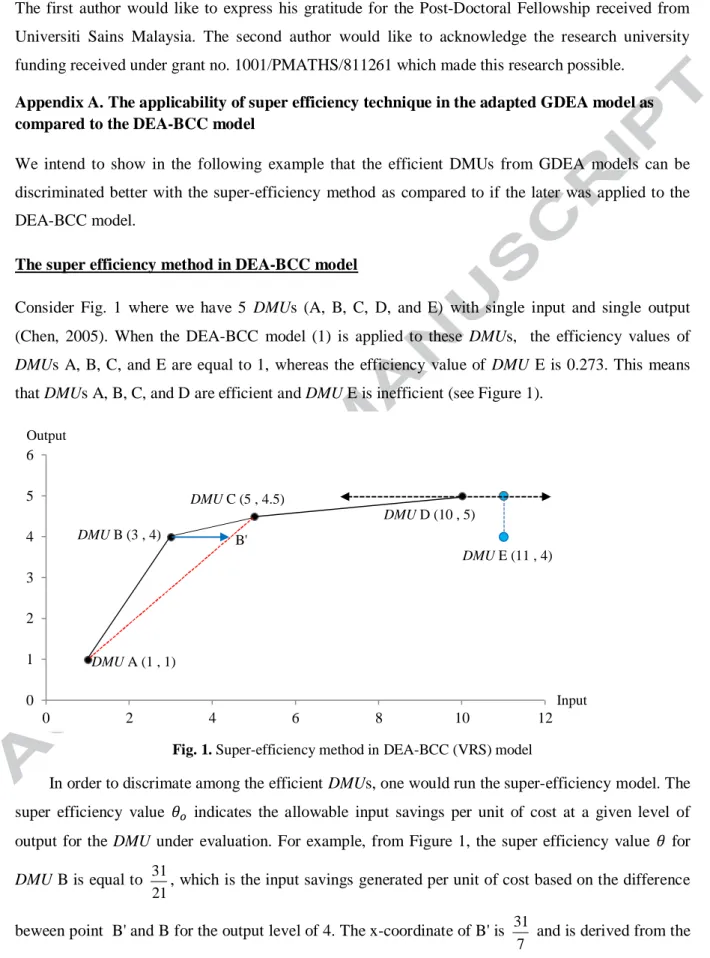
Consider Fig. 1 where we have 5 DMUs (A, B, C, D, and E) with single input and single output (Chen, 2005). When the DEA-BCC model (1) is applied to these DMUs, the efficiency values of DMUs A, B, C, and E are equal to 1, whereas the efficiency value of DMU E is 0.273. This means thatDMUs A, B, C, and D are efficient andDMU E is inefficient (see Figure 1).
Fig. 1. Super-efficiency method in DEA-BCC (VRS) model
In order to discrimate among the efficient DMUs, one would run the super-efficiency model. The super efficiency value indicates the allowable input savings per unit of cost at a given level of output for theDMU under evaluation. For example, from Figure 1, the super efficiency value for DMU B is equal to 31
21, which is the input savings generated per unit of cost based on the difference
beween point B' and B for the output level of 4. The x-coordinate of B' is 31
7 and is derived from the 0 1 2 3 4 5 6 0 2 4 6 8 10 12 DMUA (1 , 1) DMUB (3 , 4) DMUC (5 , 4.5) DMUD (10 , 5) DMUE (11 , 4) B' Input Output
convex combination of A and C indicating that the input ofDMU B has an allowable increase from 3 to 31
7 , while remaining feasible.
The higher the value of , the higher position of that DMU in the set of efficientDMUs. The super-efficiency scores ofDMUs A, B, and C are 3, 31
21, and 13
10 respectively, but there is no feasible solution for the super efficiency model (3) when evaluating DMU D. As such, could not be computed for any potential cost savings. In addition, since DMU E is inefficient, there is no possibility for a convex combination to be formed to utilize more input for output level 5.
The super efficiency technique in the adapted GDEA model
The results of super-efficiency values for the proposed GDEA model (8) ofDMUs A, B, C, and D are 14, 5.16, 1.62, and 3.5 respectively when solving for
α
= 6. Unlike the previous case of BCC-DEA (model 3), model (8) is still feasible for DMU D. This is because solving model (8) for a particular DMU does not depend on the input values of thatDMU.The problem of Figure 1 can be formulated as follow in model (8) when evaluating the super efficiency ofDMU D: maxD
(
)
. . A 6 4 9 s t D £d + u+ v ,(
)
6 7 B d u v D £ + + ,(
)
6 0.5 5 C d u v D £ + + ,(
)
6 E d u v D £ + - , 1 u- =v , , 0 u v³ ,where dA =max 4 ,9
{
u v}
, dB =max{
u, 7v}
, dC =max 0.5 , 5{
u v}
and dE =max{ }
u v, .By considering constraint u- =v 1, it can be concluded that v= -u 1. Therefore the above LP problem can be rewritten as follows:
maxD . . A 78 54 s t D £d + u- , 48 42 B d u D £ + - , 33 30 C d u D £ + - , 6 E d D £ + , 0 u³ ,
where dA =max 4 ,9
{
u u-9}
, dB =max{
u,7u-7}
, dC =max 0.5 ,5{
u u-5}
and dE =max{
u, u 1-}
.It is obvious that the above problem has a feasible solution. By solving the problem, we obtain the following solution:
1
u= and D =3.5.
It is worth noting that there are no input values of DMU D used in the above formulation. Constrastingly, model (3) is dependent on the input of the DMU under evaluation to compute the super efficiency score, which causes infeasibility problems when there are no close efficient points to form a convex combination. This is the ability of model (8) against model (3).
Appendix B.
Dataset of 23 European Union (EU) member countries (except Bulgaria, Luxembourg, Malta and Romania)
Countries Inputs Outputs
x1(thousand ton) CO2 equivalent x2 quantity of energy y1 gross electricity (%) y2( hundred million )
average annual emissions
y3 substituted fuel (%) Austria (3.853, 3.859, 4.088) (4.105, 4.130, 4.143) (59.038, 61.363, 64.980) (0.3043, 0.3088, 0.3426) 29.7 Belgium (5.482, 5.570, 5.931) (5.501, 5.567, 5.719) (3.960, 4.359, 5.391) (0.5091, 0.5231, 0.5885) 4.6 Cyprus (5.129, 5.168, 5.931) (2.503, 2.544, 2.615) (0.080, 0.105, 0.241) (0.0530, 0.0540, 0.0555) 4.6 Czech Republic (9.118, 9.143, 9.958) (4.384, 4.445, 4.545) (5.278, 5.400, 6.535) (0.7843, 0.8141, 0.8609) 8.5 Denmark (4.127, 5.369, 5.892) (3.575, 3.742, 3.828) (24.109, 26.276, 26.757) (0.2551, 0.2890, 0.2967) 9.9 Estonia (11.869, 12.645, 17.731) (4.195, 4.263, 4.361) (2.744, 2.770, 5.642) (0.1054, 0.1282, 0.1510) 22.8 Finland (8.043, 8.074, 9.179) (6.531, 6.934, 7.151) (25.214, 26.613, 30.189) (0.3793, 0.3940, 0.4073) 30.3 France (2.339, 2.355, 2.595) (4.396, 4.450, 4.468) (12.655, 13.210, 13.641) (1.2194, 1.2219, 1.3136) 12.3 Germany (5.663, 5.681, 6.609) (4.148, 4.173, 4.201) (12.144, 14.079, 15.187) (4.6013, 4.6655, 4.9795) 9.8 Greece (6.153, 6.167, 6.650) (2.807, 2.812, 2.821) (6.221, 9.788, 12.606) (0.6710, 0.6905, 0.7343) 8.2 Hungary (2.867, 2.872, 3.226) (2.698, 2.709, 2.716) (4.447, 5.026, 6.174) (0.2480, 0.2552, 0.2895) 7.7 Ireland (4.510, 4.562, 4.636) (3.664, 3.671, 3.719) (10.202, 10.817, 12.493) (0.1981, 0.2014, 0.2238) 5.0 Italy (3.377, 3.528, 3.618) (3.082, 3.114, 3.162) (15.417, 16.020, 19.090) (2.1412, 2.1485, 2.4016) 8.9 Latvia (1.646, 1.649, 1.985) (1.967, 2.018, 2.063) (40.230, 41.122, 46.793) (0.0269, 0.0276, 0.0293) 34.3 Lithuania (2.495, 3.088, 3.667) (2.594, 2.622, 2.635) (3.890, 4.590, 5.196) (0.0574, 0.0610, 0.0633) 17.0 Netherlands (5.102, 5.122, 5.552) (4.949, 5.065, 5.164) (7.060, 7.440, 8.455) (0.7804, 0.8028, 0.8203) 4.1 Poland (5.981, 5.982, 6.661) (2.449, 2.534, 2.564) (3.632, 4.112, 5.195) (2.0363, 2.0363, 2.1277) 8.9 Portugal (3.326, 3.334, 3.766) (2.349, 2.469, 2.544) (28.999, 29.543, 34.383) (0.2931, 0.3063, 0.3181) 24.5 Slovakia (5.691, 5.694, 5.904) (3.399, 3.424, 3.485) (16.570, 16.609, 18.308) (0.2352, 0.2425, 0.2689) 10.3 Slovenia (4.101, 4.266, 4.285) (3.693, 3.697, 3.836) (26.492, 28.110, 33.534) (0.0856, 0.0870, 0.0927) 16.9 Spain (3.548, 3.683, 3.805) (3.230, 3.260, 3.356) (19.523, 20.841, 24.492) (1.6183, 1.6667, 1.8543) 13.3 Sweden (2.418, 2.421, 2.594) (5.417, 5.544, 5.597) (49.794, 52.610, 53.601) (0.1852, 0.1912, 0.2095) 47.3 United Kingdom (3.453, 3.467, 3.501) (3.671, 3.724, 3.764) (5.063, 5.356, 6.250) (2.4735, 2.5119, 2.7460) 2.9
Note:Data from x1, y2 are gathered from Carbonmarketdata.com, whereas European commission’s Eurostat is the source for variables x2, y1 and y3. The data has been scaled for the population size of each country gathered from the United Nations Department of Economic and Social Affairs. Intelligent Insights International provide a compilation of sources to validate the above variables.
References
Ahn, T., Charnes, A., & Cooper, W. W. (1988). Efficiency characterizations in different DEA models. Socio-Economic Planning Sciences, 22(6), 253-257.
Andersen, P., & Petersen, N. C. (1993). A procedure for ranking efficient units in data envelopment analysis.Management Science, 39(10), 1261-1264.
Azadeh, A., Moghaddam, M., Asadzadeh, S. M., & Negahban, A. (2011). An integrated fuzzy simulation-fuzzy data envelopment analysis algorithm for job-shop layout optimization: The case of injection process with ambiguous data.European Journal of Operational Research, 214(3), 768-779.
Azadeh, A., Sheikhalishahi, M., & Asadzadeh, S. M. (2011). A flexible neural network-fuzzy data envelopment analysis approach for location optimization of solar plants with uncertainty and complexity. Renewable Energy, 36(12), 3394-3401.
Bagherzadeh valami, H. (2009). Cost efficiency with triangular fuzzy number input prices: An application of DEA.Chaos, Solitons & Fractals, 42(3), 1631-1637.
Banker, R. D., Charnes, A., & Cooper, W. W. (1984). Some models for estimating technical and scale inefficiencies in data envelopment analysis.Management Science, 30(9), 1078-1092.
Charnes, A., Cooper, W. W., & Rhodes, E. (1978). Measuring the efficiency of decision making units.European Journal of Operational Research, 2(6), 429-444.
Chen, Y. (2005). Measuring super-efficiency in DEA in the presence of infeasibility. European Journal of Operational Research, 161(1), 447-468.
Cook, W. D., Liang, L., Zha, Y., & Zhu, J. (2008). A modified super-efficiency DEA model for infeasibility.Journal of the Operational Research Society, 60(2), 276-281.
Cooper, W. W., Seiford, L. M., & Tone, K. (2007). Data envelopment analysis: A comprehensive text with models, applications, references and DEA-Solver Software. Second editions.Springer, ISBN, 387452818, 490.
Deprins, D., Simar, L., & Tulkens, H. (1984).Measuring labor-efficiency in post offices (M. Marchand, P. Pestieau, H. Tulkens ed.). North-Holland, Amsterdam: The Performance of Public Enterprises: Concepts and Measurment Emrouznejad, A. & M. Tavana (2014). Performance Measurement with Fuzzy Data Envelopment Analysis. In the series of
“Studies in Fuzziness and Soft Computing”, Springer-Verlag, ISBN 978-3-642-41371-1.
Ghasemi, M. R., Ignatius, J., & Davoodi, S. M. (2014a). Ranking of Fuzzy Efficiency Measures via Satisfaction Degree. In Performance Measurement with Fuzzy Data Envelopment Analysis (pp. 157-165). Springer Berlin Heidelberg. Ghasemi, M. R., Ignatius, J., & Emrouznejad, A. (2014b). A bi-objective weighted model for improving the discrimination
power in MCDEA.European Journal of Operational Research,233(3), 640-650.
Guo, P., & Tanaka, H. (2001). Fu