Modeling model uncertainty

(1)

WORKING PAPER NO. 169

MODELING

MODEL UNCERTAINTY

BY ALEXEI ONATSKI

AND NOAH WILLIAMS

E U R O P E A N C E N T R A L B A N K

WORKING PAPER SERIES

INTERNA TIONAL SEMINAR ON MA CR_OECONOMICS

(2)

WORKING PAPER NO. 169

MODELING

MODEL UNCERTAINTY

BY ALEXEI ONATSKI

*

AND NOAH WILLIAMS

**

August 2002

E U R O P E A N C E N T R A L B A N K

WORKING PAPER SERIES

INTERNA TIONAL SEMINAR ON MA CR_OECONOMICS

(3)

Address Kaiserstrasse 29

D-60311 Frankfurt am Main Germany

Postal address Postfach 16 03 19

D-60066 Frankfurt am Main Germany Telephone +49 69 1344 0 Internet http://www.ecb.int Fax +49 69 1344 6000 Telex 411 144 ecb d

Reproduction for educational and non-commercial purposes is permitted provided that the source is acknowledged. The views expressed in this paper are those of the authors and do not necessarily reflect those of the European Central Bank.

(4)

Recently there has been much interest in studying monetary policy under model uncertainty. We develop methods to analyze different sources of uncertainty in one coherent structure useful for policy decisions. We show how to estimate the size of the uncertainty based on time series data, and incorporate this uncertainty in policy optimization. We propose two different approaches to modeling model uncertainty. The first is model error modeling, which imposes additional structure on the errors of an estimated model, and builds a statistical description of the uncertainty around a model. The second is set membership identification, which uses a deterministic approach to find a set of models consistent with data and prior assumptions. The center of this set becomes a benchmark model, and the radius measures model uncertainty. Using both approaches, we compute the robust monetary policy under different model uncertainty specifications in a small model of the US economy.

JEL Classiﬁcations: E52, C32, D81.

(6)

Non-technical Summary

Uncertainty is pervasive in economics, and this uncertainty must be faced continually by policy makers. In this paper we propose empirical methods to specify and measure uncer-tainty associated with economic models, and we study the effects of unceruncer-tainty on monetary policy decisions. Recently there has been a great deal of research activity on monetary policy making under uncertainty. We add to this literature by developing new, coherent methods to quantify uncertainty and to tailor decisions to the empirically relevant sources of uncertainty. In particular, we will be concerned with four types of uncertainty: first, uncertainty about parameters of a reference model (including uncertainty about the model’s order); second, un-certainty about the spectral characteristics of noise; third, unun-certainty about data quality; and fourth, uncertainty about the reference model itself. We use a simple, empirically-based macroeconomic model in order to analyze the implications of uncertainty for economic policy. A common intuitive view is that the introduction of uncertainty should make policy makers cautious. However, uncertainty need not result in cautiousness. Further, different assumptions about the structure of uncertainty have drastically different implications for policy activism. In our view, the most important message of the fragility of the robust rules found in the literature is that to design a robust policy rule in practice, it is necessary to combine different sources of uncertainty in a coherent structure and carefully estimate or calibrate the size of the uncertainty. Further, the description and analysis of uncertainty should reflect the use of the model for policy purposes. For these reasons, it is necessary to

model the model uncertainty.

In this paper we consider two particular ways to structure and estimate the model uncer-tainty. First, we consider the Model Error Modeling (MEM) approach as in Ljung (1999). The main idea of the approach is as follows. First, estimate a reference or nominal model. Then take the reference model’s errors and try to ﬁt them with a general set of explana-tory variables (including some variables omitted from the original model). Finally, build the model uncertainty set around the reference model which is consistent with all regressions for the errors not rejected by formal statistical procedures.

The second approach exploits recent advances in the Set Membership (SM) identification literature, due to Milanese and Taragna (2001). Set membership theory takes a deterministic approach to model uncertainty. The uncertainty corresponds to an infinite number of linear constraints on the model’s parameters and shocks. The model uncertainty set is represented by those models that are not falsified by the data and the above linear restrictions. The SM approach makes very few a priori assumptions about the model’s shocks and parameters. While this generality is a benefit of the approach, it implies that the resulting uncertainty set may be very large and complicated. To make it operational, it is modeled (approximated) by a ball in the model space that covers the uncertainty set and has minimal radius among all such balls. The center of this ball serves as the nominal model. Thus this approach provides both an estimate of a nominal model and a description of the model uncertainty, based entirely on the specified assumptions and the observed data.

After a model of the model uncertainty is built (under either approach), the robust policy is formulated so that it works well for all models described by this model uncertainty

(7)

model. In order to guarantee theuniform performance across the different models, following much of the recent literature, we use a minimax approach to formulating robust policies. The general message of our results is that there is substantial uncertainty in a class of simple models used for monetary policy. Further, different ways of modeling uncertainty can lead to quite different outcomes. In the MEM approach we find that, of the different sources of uncertainty, model uncertainty has the largest effect on losses, the real-time data uncertainty is less dangerous for policy making, whereas the effects of pure shock uncertainty are relatively mild. While the full estimated model of uncertainty is too large to guarantee finite losses for any Taylor-type rules, we are able to find the rules optimally robust against specific blocks of the uncertainty model taken separately. We find that almost all computed robust rules are relatively more aggressive than the optimal rule under no uncertainty.

Under the SM approach, we develop an estimation procedure that minimizes a measure of model uncertainty. We analyze two sets ofa priori assumptions, and find that the estimates and the evaluation of uncertainty differ dramatically. In all cases, the amount of uncertainty we estimate is substantial, and tends to be concentrated at high frequencies. Further, the models we estimate imply substantially different inflation dynamics than a conventional OLS estimate. We find that the resulting robust Taylor rules respond more aggressively to both inflation and the output gap relative to the optimal Taylor rules under no uncertainty.

Under both of our approaches the most damaging perturbations of the reference model result from very low frequency movements. Since we impose a vertical long run Phillips curve, increases in the output gap lead to very persistent increases in inﬂation under relatively non-aggressive interest rate rules. The size of this persistent component is poorly measured, but has a huge impact on the losses sustained by the policy maker. We believe that for practical purposes, it is prudent to downweight the importance of the low frequency movements. The baseline model that we use, is essentially an aggregate demand-aggregate supply model. Such models are not designed to capture long-run phenomena, but are instead most appropriately viewed as short-run models of ﬂuctuations.

To tailor our uncertainty description to more relevant worst scenarios, we reconsider our results when restricting our attention to business cycle frequencies. For both MEM and SM approaches, our aggressiveness result becomes reversed. Now, almost all optimally robust Taylor rules are less aggressive than the optimal Taylor rules under no uncertainty. The worst case scenarios across all frequencies correspond to cases when inflation gradually grows out of control. Therefore the robust rules respond aggressively to any signs of inflation in order to fight off this possibility. However when we introduce model uncertainty at business cycle frequencies only, then the worst case scenarios occur at these frequencies, and the policy is very responsive to these frequencies. This comes at the cost of downweighting low frequency movements. Instead of fighting off any incipient inflation, policy becomes less aggressive, and focuses more on counter-cyclical stabilization policy. This contrasts with policymakers worried about low frequency perturbations, who would be very reluctant to try to stimulate the economy in a recession.

(8)

1 Introduction

Uncertainty is pervasive in economics, and this uncertainty must be faced continually by policy makers. In this paper we propose empirical methods to specify and measure uncer-tainty associated with economic models, and we study the effects of unceruncer-tainty on monetary policy decisions. Recently there has been a great deal of research activity on monetary policy making under uncertainty. We add to this literature by developing new, coherent methods to quantify uncertainty and to tailor decisions to the empirically relevant sources of uncertainty. In particular, we will be concerned with four types of uncertainty: first, uncertainty about parameters of a reference model (including uncertainty about the model’s order); second, un-certainty about the spectral characteristics of noise; third, unun-certainty about data quality; and fourth, uncertainty about the reference model itself. We use a simple, empirically-based macroeconomic model in order to analyze the implications of uncertainty for economic policy. A common intuitive view is that the introduction of uncertainty should make policy makers cautious. This view reflects the results of Brainard (1967), which Blinder (1997) summarizes as “Brainard’s conservatism principle: estimate what you should do, and then do less.” However, as was argued by Chow (1975) from the theoretical point of view, uncer-tainty need not result in cautiousness.1 Even the notion of aggressiveness of policy depends on the policy instrument. An aggressive interest rate rule is compatible with an attenu-ated money growth rule, and vice versa. However most recent studies on the robustness of monetary policy under uncertainty have focused on interest rate rules, and have typically found aggressive policy rules. The idea is that some types of uncertainty mean that policy instruments may turn out to have weaker effects than expected, which can in turn lead to large potential losses. In these cases, it is optimal to react more aggressively with uncer-tainty than without. Despite these exceptions, the conservatism principle appeals to many, perhaps not least because empirically estimated interest rate rules are typically found to be less aggressive than theoretically optimal rules.

Different assumptions about the structure of uncertainty have drastically different impli-cations for policy activism. For example, introduction of an extreme shock uncertainty into the Ball (1999) model, so that the serial correlation structure of the shocks is not restricted in any way (see Sargent (1999)), implies an aggressive robust Taylor rule.2 On the contrary, Rudebusch (2001) shows that focusing on the real time data uncertainty in a conceptually similar Rudebusch and Svensson (1999) model leads to attenuation of the parameters of the optimal Taylor rule. Further, Craine (1979) and Söderström (2002) show that uncer-tainty about the dynamics of inflation leads to aggressive policy rules. Finally, Onatski and Stock (2002) find that uncertainty about the lag structure of the Rudebusch-Svensson model requires a cautious reaction to inflation but an aggressive reaction to the output gap.

The fact that the robust policy rules are so fragile with respect to diﬀerent assumptions

1_{Although the conservatism result is better known, Brainard (1967) also notes that a large enough} co-variance between the shocks and (random) parameters can lead policy to be more aggressive.

2_{The robust rule is deﬁned as the policy rule that minimizes losses under the worst possible scenario} consistent with the uncertainty description.

(9)

about the structure of uncertainty is not surprising by itself. In fact, fragility is a general feature of optimizing models. As Carlson and Doyle (2002) state, “They are ‘robust, yet fragile’, that is, robust to what is common or anticipated but potentially fragile to what is rare or unanticipated.” Standard stochastic control methods are robust to realizations of shocks, as long as the shocks come from the assumed distributions and feed through the model in the specified way. But the optimal rules may perform poorly when faced with a different shock distribution, or slight variation in the model. The Taylor policy rules discussed above are each designed to be robust to a particular type of uncertainty, but may perform poorly when faced with uncertainty of a different nature.

In our view, the most important message of the fragility of the robust rules found in the literature is that to design a robust policy rule in practice, it is necessary to combine different sources of uncertainty in a coherent structure and carefully estimate or calibrate the size of the uncertainty. Further, the description and analysis of uncertainty should reflect the use of the model for policy purposes. Model selection and evaluation should not be based only on the statistical fit or predictive ability of the model, but should be tied to the ultimate policy design objectives. For these reasons, it is necessary to model the model uncertainty.

It is sometimes argued that model uncertainty can be adequately represented by suitable restrictions on the joint distribution of shocks only. We argue that, if the model uncertainty is used to formulate a robust policy rule, the distinction between restrictions on the vector of model parameters and the distribution of shocks may be crucial. In particular, we develop an example showing that the Hansen and Sargent (2002) approach to formulating model uncertainty may lead to the design of robust policy rules that can be destabilized by small parametric perturbations. This potential inconsistency between the robustness to shock uncertainty and the robustness to parametric uncertainty results from the fact that the magnitude of the shock uncertainty relevant for policy evaluation cannot be judgedex ante, but depends on the policy being analyzed. For example, uncertainty about the slope of the IS curve is equivalent to larger shocks under more aggressive interest rate rules.

In this paper we consider two particular ways to structure and estimate the model uncer-tainty. Both draw upon the recent advances in the control system identiﬁcation literature. First, we consider the Model Error Modeling (MEM) approach as in Ljung (1999). The main idea of the approach is as follows. First, estimate a reference or nominal model. Then take the reference model’s errors and try to ﬁt them with a general set of explanatory variables (including some variables omitted from the original model). Finally, build the model uncer-tainty set around the reference model which is consistent with all regressions for the errors not rejected by formal statistical procedures.

The second approach exploits recent advances in the Set Membership (SM) identification literature, due to Milanese and Taragna (2001). Set membership theory takes a deterministic approach to model uncertainty. The uncertainty corresponds to an infinite number of linear constraints on the model’s parameters and shocks. Typically, shocks are required to be bounded in absolute value by a given positive number and the model impulse responses are required to decay at a given exponential rate. The model uncertainty set is represented by those models that are not falsified by the data and the above linear restrictions. The SM

(10)

approach makes very few a priori assumptions about the model’s shocks and parameters. While this generality is a beneﬁt of the approach, it implies that the resulting uncertainty set may be very large and complicated. To make it operational, it is modeled (approximated) by a ball in the model space that covers the uncertainty set and has minimal radius among all such balls. The center of this ball serves as the nominal model. Thus this approach provides both an estimate of a nominal model and a description of the model uncertainty, based entirely on the speciﬁed assumptions and the observed data.

After a model of the model uncertainty is built (under either approach), the robust policy is formulated so that it works well for all models described by this model uncertainty model. In order to guarantee theuniform performance across the diﬀerent models, following much of the recent literature, we use a minimax approach to formulating robust policies. Although an alternative Bayesian approach has strong theoretical foundations, it is less tractable computationally. Further, minimax policies have alternative theoretical foundations and they are naturally related to some of our estimation methods.3 An interesting extension of our results would be use our measures of model uncertainty as a basis for Bayesian optimal control, and to compare Bayes and minimax policy rules.

Under both the model error modeling and set membership approaches, a certain level of subjectivity exists at the stage of formulating the model of model uncertainty. In the MEM approach, one has to choose a set of explanatory variables for the model of errors and the level of statistical tests rejecting those models inconsistent with the data. In the SM approach, it is necessary to specify a priori a bound on absolute value of the shocks and the rate of exponential decay of the impulse responses. There are no clear guidelines in making these subjective choices. If one wants to decrease subjectivity, one is forced to consider more and more general models of the model errors or, in the set membership case, less and less restrictive assumptions on the rate of decay and the shock bound. However, an eﬀect of such vagueness may be an enormous increase in the size of the uncertainty.

One possible way to judge the specification of model uncertainty models is to do some ex-post analysis and examination. The end results of our procedures are robust Taylor-type rules and guaranteed upper bounds on a quadratic loss function. One procedure for assessing the specification of model uncertainty models would be to see if the bounds on the loss function or the robust rules themselves satisfy some criterion of “reasonability.” Another procedure which Sims (2001) suggests would be to examine in more detail the implied worst-case model which results from the policy optimization, to see if it implies plausible prior beliefs. By doing this ex-post analysis, the specifications could be tailored or the results from different specifications could be weighted. Our results should prepare the reader to carry out this task by incorporating his own subjective beliefs.

The general message of our results is that there is substantial uncertainty in a class of simple models used for monetary policy. Further, diﬀerent ways of modeling uncertainty can lead to quite diﬀerent outcomes. As an illustration of our methods, we analyze the uncertainty in the Rudebusch and Svensson (1999) model. This provides an empirically

3_{Gilboa and Schmeidler (1989) provide an axiomatic foundation for max-min expected utility. While we} share a similar approach, their setting diﬀers from ours.

(11)

relevant, but technically simple laboratory to illustrate the important features of our analysis. Further, we impose relatively few restrictions on the form of the model uncertainty. Much more could be done to extend the baseline model we use (for example to consider forward-looking behavior) and to use prior beliefs to further restrict the classes of models we consider (for example by imposing sign restrictions on impulse responses). This paper is only a first step in the analysis, but even by focusing on a simple case we find some interesting results. We first assess the different sources of uncertainty in the Rudebusch and Svensson (1999) model under our Model Error Modeling approach. We find that the famous Taylor (1993) rule leads to extremely large losses for very small perturbations. Of the different sources of uncertainty, model uncertainty has the largest effect on losses, the real-time data uncer-tainty is less dangerous for policy making, whereas the effects of pure shock unceruncer-tainty are relatively mild. While the full estimated model of uncertainty is too large to guarantee finite losses for any Taylor-type rules, we are able to find the rules optimally robust against specific blocks of the uncertainty model taken separately. We find that almost all computed robust rules are relatively more aggressive than the optimal rule under no uncertainty. An exception to this aggressiveness result is the rule robust to the real-time data uncertainty about the output gap. This rule is substantially less aggressive than the optimal rule under no uncertainty, which accords with results of Rudebusch (2001).

Under the Set Membership approach, we assess the uncertainty of different parametric models, and develop an estimation procedure that minimizes a measure of model uncertainty. We analyze two sets ofa priori assumptions, and find that the estimates and the evaluation of uncertainty differ dramatically. In all cases, the amount of uncertainty we estimate is substantial, and tends to be concentrated at high frequencies. Further, the models we estimate imply substantially different inflation dynamics than a conventional OLS estimate. In order to obtain reasonable policy rules, for some specifications we must scale down the model uncertainty in the different estimates. We find that the resulting robust Taylor rules respond more aggressively to both inflation and the output gap relative to the optimal Taylor rules under no uncertainty.4

Under both of our approaches the most damaging perturbations of the reference model result from very low frequency movements. Since we impose a vertical long run Phillips curve, increases in the output gap lead to very persistent increases in inﬂation under rel-atively non-aggressive interest rate rules. The size of this persistent component is poorly measured, but has a huge impact on the losses sustained by the policy maker. We believe that for practical purposes, it is prudent to downweight the importance of the low frequency movements. The baseline model that we use, due to Rudebusch and Svensson (1999), is essentially an aggregate demand-aggregate supply model. Such models are not designed to capture long-run phenomena, but are instead most appropriately viewed as short-run models of ﬂuctuations. By asking such a simple model to accommodate very low frequency pertur-bations, we feel that we are pushing the model too far. A more fully developed model is

4_{Due to technical constraints spelled out in the paper, we analyze only uncertainty about the Phillips} curve under the SM approach. Neither the real-time data uncertainty, nor uncertainty about the IS curve are considered.

(12)

necessary to capture low frequency behavior.

To tailor our uncertainty description to more relevant worst scenarios, we reconsider our results when restricting our attention to business cycle frequencies (corresponding to periods from 6 to 32 quarters). For both MEM and SM approaches, our aggressiveness result becomes reversed. Now, almost all optimally robust Taylor rules are less aggressive than the optimal Taylor rules under no uncertainty. For the MEM approach, the least aggressive robust rule corresponds to the uncertainty about the slope of the IS curve and not to the real-time data uncertainty about the output gap. The full estimated uncertainty model is still too big to allow for finite worst possible losses under any Taylor-type rule, however, when we scale the size of all uncertainty downwards, the optimally robust Taylor rule has a coefficient on inflation of 1.4 and a coefficient on the output gap of 0.7, which is surprisingly close to the Taylor (1993) rule! For the SM approach, our estimated model can handle the full estimated uncertainty, and it also leads to a relatively less aggressive policy rule.

These results can be interpreted as follows. Under no model uncertainty, the optimal Taylor-type rules balance the performance of policy at all frequencies. When we introduce model uncertainty which enters at all frequencies, the most damaging perturbations come at low frequencies. Thus the robust optimal rules pay a lot of attention to these frequencies, at the cost of paying less attention to other frequencies. The worst case scenarios correspond to cases when inflation gradually grows out of control. Therefore the robust rules respond aggressively to any signs of inflation in order to fight off this possibility. However when we introduce model uncertainty at business cycle frequencies only, then the worst case scenarios occur at these frequencies, and the policy is very responsive to these frequencies. This comes at the cost of downweighting low frequency movements, even relative to the no uncertainty case. Instead of fighting off any incipient inflation, policy becomes less aggressive, and focuses more on counter-cyclical stabilization policy. This contrasts with policymakers worried about low frequency perturbations, who would be very reluctant to try to stimulate the economy in a recession.

Two recent studies are particularly relevant for the Model Error Modeling part of our paper. Rudebusch (2001) analyzes optimal policy rules under different changes in specifica-tion of the Rudebusch-Svensson model. In this paper, we find minimax, not Bayes optimal, policy rules corresponding to different specifications of uncertainty. Further, the uncertainty we consider is more general than in Rudebusch (2001). Onatski and Stock (2002) analyze stability robustness of Taylor-type policy rules in the Rudebusch-Svensson model. Here we extend their analysis in a number of important ways. First, we study robust performance of the policy rules. We compute optimally robust policy rules and not just sets of the rules not destabilizing the economy that were computed in Onatski and Stock. Moreover, our more precise analysis makes it possible to study combined model, real-time data, and shock uncertainty in one structure. Second, we carefully calibrate the magnitude of the uncertainty about the Rudebusch-Svensson model using Bayesian estimation techniques.

To our knowledge, there are no previous attempts to estimate economic models with a goal of minimizing model ambiguity. This is essentially what we do in the part of the paper concerned with the Set Membership identiﬁcation. Chamberlain (2000) uses max-min

(13)

expected utility theory in estimation, but considers parametric estimation with a given set of possible models. In contrast, a main task of our analysis is to construct an empirically plausible model set. Other broadly related papers use the theory of information based com-plexity, which is a general theory from which SM is derived. Information based complexity theory has been used and extended in economics by Rust (1997) and Rust, Traub, and Wozniakowski (2002) to study the numerical solution of dynamic programming problems.

In the next section of the paper we describe formulations of models of model uncertainty at a formal level, and show that parametric and shock uncertainty must be considered separately. Section 3 applies the Model Error Modeling approach to analyze robust monetary policies under uncertainty about Rudebusch-Svensson model. Section 4 models the Phillips curve and uncertainty associated with it using the Set Membership identiﬁcation approach. Section 5 concludes.

2 Consequences of Diﬀerent Uncertainty Models

2.1 Overview

The general issue that we consider in this paper is decision making under uncertainty. In particular, we focus on the policy-relevant problem of choosing interest rate rules when the true model of the economy is unknown and may be subject to diﬀerent sources of uncertainty. The goal of the paper is to provide characterizations of the empirically relevant sources of uncertainty, and to design policy rules which account for that uncertainty.

As we noted in the introduction, we distinguish between diﬀerent sources of uncertainty, each of which can lead to diﬀerent implications for policy rules. To be concrete, it helps to introduce a standard state-space model:

xt+1 = Axt+Bit+Cεt+1 (1)

y_t = Dx_t+Gi_t+F η_t z_t = Hx_t+Ki_t

Herex_t is a vector state variables,i_t is a vector of controls, ε_t is a driving shock vector,y_tis a vector of observations, η_t is an observation noise and z_t is a vector of target variables. In the standard full information case, F = 0. By model uncertainty we mean uncertainty both about the parameters of the model and the model specification. In (1) this means variations in the A and B matrices (parametric uncertainty) as well as the makeup of the x_t vector (perhaps it omits relevant variables). By shock uncertainty we mean uncertainty about the serial correlation properties of the noise ε_t. By data uncertainty we mean uncertainty about the real-time data generating process. We capture this uncertainty by allowing variation in matrices D and G and specifying a range of possible spectral characteristics of η_t. Each of these sources of uncertainty enters the model (1) in a different way and can therefore lead to different outcomes.

One approach to model uncertainty which has been widely used was developed by Hansen and Sargent (2002). They absorb all sources of uncertainty into an additional shock to the

(14)

system, and therefore collapse all uncertainty into shock uncertainty. Focusing on the full information case, they suppose that the ﬁrst line of (1) is replaced by:

x_t₊₁ = Ax_t+Bi_t+C(ε_t₊₁+w_t₊₁). (2) The decision maker then designs a control strategy that will be insensitive to sequences of w_t of a reasonable size (described in more detail below). While this approach seems quite general and unrestrictive, in the next section we develop a simple example which shows that the other sources of uncertainty cannot be collapsed to shock uncertainty.

To gain some intuition for the results, suppose that the decision maker uses a feedback control rulei_t=kx_t, and for simplicity assume C is the identity matrix. Then (2) becomes:

x_t₊₁ = (A+Bk)x_t+ε_t₊₁+w_t₊₁.

Next, suppose that the true data generating process was a purely parametric perturbation of (1), so that Ais replaced by A+ Â, andB byB+ ˆB. In this case we have that the model uncertainty perturbation is w_t₊₁ = ( Â+ ˆBk)x_t, which clearly varies with the control rulek. Therefore in this setting it is impossible to evaluate the model uncertainty in the absence of the control rule. Different control rules will lead to different magnitudes of uncertainty, which cannot be judged ex-ante. This intuition is made more precise in the following section.

2.2 A Simple Example

In this section we build an example showing that two reasonable views of model uncertainty in a small macroeconometric model of the US economy may lead to drastically diﬀerent policy implications. We consider a two-equation purely backward-looking model of the economy proposed and estimated by Rudebusch and Svensson (1999). This model, henceforth referred to as RS, will be the benchmark for the rest of the paper as well, and is given by:

π_t₊₁ = .70

(.08)πt−(..1010)πt−1+(..2810)πt−2+(..1208)πt−3+(..1403)yt+επ,t+1 (3)

y_t₊₁ = 1.16

(.08)yt−(..2508)yt−1−(..1003)(¯ıt−π¯t) +εy,t+1

The standard errors of the parameter estimates are given in parentheses. Here the variable y stands for the gap between output and potential output,π is inﬂation andi is the federal funds rate. All the variables are quarterly, measured in percentage points at an annual rate and demeaned prior to estimation, so there are no constants in the equations. Variables π and i stand for four-quarter averages of inﬂation and federal funds rate respectively.

The first equation is a simple version of the Phillips curve. The coefficients on the lags of inflation in the right hand side of the equation sum to one, so that the Phillips curve is vertical in the long run. The second equation is a variant of the IS curve. A policy maker can control the federal funds rate and wants to do so in order to keep yand π close to their target values (zero in this case).

(15)

In general, the policy maker’s control may take the form of a contingency plan for her future settings of the federal funds rate. We, however, will restrict attention to the Taylor-type rules for the interest rate. As emphasized by McCallum (1988) and Taylor (1993), simple rules have the advantage of being easy for policymakers to follow and also of being easy to interpret. In this section, we will assume that the policy maker would like to choose among the following rules:

i_t =g_ππ¯_t₋₁+g_yy_t₋₂ (4) Here, the interest rate reacts to both inﬂation and the output gap with delay. The delay in the reaction to the output gap is longer than that in the reaction to the inﬂation because it takes more time to accurately estimate the gap.

Following Rudebusch and Svensson, we assume that a policy maker has the quadratic loss:5

L_t = ¯π_t2+y_t2+1

2(it−it−1)

2_. ₍₅₎

Had the policy maker been sure that the model is correctly specified, she could have used standard frequency-domain methods to estimate expected loss for any given policy rule (4). Then she could find the optimal rule numerically. We will however assume that the policy maker has some doubts about the model. She wants therefore to design her control so that it works well for reasonable deviations from the original specification.

One of the most straightforward ways to represent her doubts is to assume that the model parameters may deviate from their point estimates as, for example, is assumed in Brainard (1967). It is also likely, that the policy maker would not rule out misspeciﬁcations of the model’s lag structure. As Blinder (1997) states, “Failure to take proper account of lags is, I believe, one of the main sources of central bank error.”

For the sake of illustration, we will assume that the policy maker is willing to contemplate a possibility that one extra lag of the output gap in the Phillips curve and IS equations and one extra lag of the real interest rate in the IS equation were wrongfully omitted in the original model. She therefore re-estimates the RS model with the additional lags. The re-estimated model has the following form:

πt+1 = .70

(.08)πt−(..1010)πt−1+(..2810)πt−2+(..1209)πt−3 +(..1410)yt+(..0010)yt−1+επ,t+1 (6)

y_t₊₁ = 1.13

(.08)yt−(..0812)yt−1−(..1408)yt−2−(..3214)(¯ıt−π¯t) +(..2414)(¯ıt−1−π¯t−1) +εy,t+1

Then she obtains the covariance matrix of the above point estimates and tries to design her control so that it works well for reasonable deviations of the parameters from the point estimates. For example, she may consider all parameter values inside the 90% conﬁdence ellipsoid around the point estimates.6

5_{Inclusion of the term (}_i

t−it−1)2 in the loss function is somewhat controversial. Our results will not depend on whether this term is included in the loss function or not.

6_{In the later sections of the paper we will discuss a more systematic way of representing and estimating} the model uncertainty.

(16)

Technically, the above control design problem may be hard (because of the large num-ber of parameters), but conceptually, it is straightforward. We will soon return to this problem, but for now let us assume that the policy maker considers a diﬀerent, more manageable, representation of the model uncertainty. Therefore she applies the Hansen and Sargent (2002) approach described above. For our example, the elements of (1) are x_t = (π_t, π_t₋₁, π_t₋₂, π_t₋₃, y_t, y_t₋₁, i_t₋₁, i_t₋₂, i_t₋₃), y_t = x_t (the state of the economy is per-fectly observable), ε_t = επt √ V arεπt, εyt √ V arεyt , and z_t = π_t, y_t,it−√it−1 2 .

As we note above, under this approach the policy maker wants to choose rules which are insensitive to the distortion w_t in (2). More precisely, the policy maker solves the following problem: min F max{wt} E ∞ t=0 βtz_tz_t s.t. (2) and E ∞ t=0 βtw_tw_t< η. (7) The minimum is taken over all policies from the admissible set F (set of policy rules (4) in our example), the parameter η regulates the size of the model uncertainty, and β is a discount factor. Here we consider the case β →1.

Problem (7) can be stated in an equivalent form min F max{wt} E ∞ t=0 βtz_tzt−θβtwtwt s.t. (2), (8)

whereθ is the Lagrange multiplier on the constraint in (7). A smaller value ofθ corresponds to stronger preference for robustness as described in Hansen and Sargent (2002). Giordani and S¨oderlind (2002) explain how to solve this problem numerically for any given value ofθ. Anderson, Hansen, and Sargent (2000) propose to discipline the choice ofθby computing the Bayesian probability of error in distinguishing between the reference model (1) and the distorted model (2), both controlled by the robust rule corresponding to θ. If the detection error probability is large, say larger than 0.1, the models are diﬃcult to statistically distin-guish from each other and the robustness parameter θ is said to correspond to a reasonable degree of model uncertainty. We will not calibrate θ using the detection error probabilities, but instead takeθ to be the smallest robustness parameter such that there exists a rule from

F corresponding to a ﬁnite value of problem (8). In other words, we ﬁnd a Taylor-type policy rule that “works best” when the size of the model uncertainty, η, increases.

It can be shown that the robust policy rule corresponding to the “smallest possible” θ minimizes the so-called H_∞ norm of the closed loop system transforming the noise ε into the target variables z (see Hansen and Sargent (2002)). It is therefore easy to ﬁnd such an “extremely robust” rule numerically using, for example, commercially available Matlab codes to compute the H_∞ norm. Our computations give the following rule:

i_t = 3.10¯π_t₋₁+ 1.41y_t₋₂. (9) Now let us return to our initial formulation of the problem. Recall that originally we wanted to ﬁnd a policy rule that works well for all deviations of the parameters of the re-estimated model (6) inside a 90% conﬁdence ellipsoid around the point estimates. Somewhat

(17)

surprisingly, the above “extremely robust” rule does not satisfy our original criterion for robustness. In fact, it destabilizes the economy for deviations from the parameters’ point estimates inside as small as a 20% conﬁdence ellipsoid. More precisely, policy rule (9) results in inﬁnite expected loss for the following perturbation of the RS model:

π_t₊₁ = .68π_t−.13π_t₋₁ +.35π_t₋₂+.10π_t₋₃+.30y_t−.15y_t₋₁+ε_π,t₊₁ (10) y_t₊₁ = 1.15y_t−.07y_t₋₁ −.18y_t₋₂−.51 (¯ı_t−π¯_t) +.41 (¯ı_t₋₁−π¯_t₋₁) +ε_y,t₊₁.

Let us denote the independent coeﬃcients7 of the above model, the re-estimated the RS model (6), and the original RS model as c, c₁, and c₀ respectively.8 Denote the covariance matrix of the coeﬃcients in the re-estimated model (6) as V. Then we have:

(c−c₁)V−1(c−c₁) = 6.15 (c₀−c₁)V−1(c₀−c₁) = 5.34.

Both numbers are smaller than the 20% critical value of the chi-squared distribution with 10 degrees of freedom. This may be interpreted as saying that both the original Rudebusch-Svensson model and the perturbed model are statistically close to the encompassing re-estimated model.

Why does our “extremely robust” rule perform so poorly? It is not because other rules work even worse. For example, we numerically checked that the famous Taylor rule i_t = 1.5¯π_t₋₁ + 0.5y_t₋₂ guarantees stability of the economy at least for all deviations inside a 60% confidence ellipsoid. Rule (9) works so bad simply because it was not designed to work well in such a situation. To see this, note that our original description of the model uncertainty allowed deviations of the slope of the IS curve from its point estimate. Therefore our ignorance about this parameter will be particularly influential if we were to use a very aggressive control rule. It may even be consistent with instability under such an aggressive rule. No effects of this kind are allowed under the Hansen and Sargent (2002) description of the model uncertainty. Under this description, ignorance is equally influential for any policy rules. The specific interaction between the aggressiveness of policy rules and uncertainty about the slope of the IS curve is not taken into account. This lack of structure in the uncertainty description turns out to be dangerous because the resulting robust rule happens to be quite aggressive.

The example just considered should not be interpreted in favor of a particular description of uncertainty. Its message should rather be understood as follows. When designing robust policy rules we must carefully specify and thoroughly understand the model uncertainty that we are trying to deal with. Robust policy rules may be fragile with respect to reasonable changes in the model uncertainty specification. In the next sections therefore we try to rigorously approach the specification of the model uncertainty. We first use an approach

7_{Recall that the sum of coefficients on inflation in the Phillips curve is restricted to be equal to 1. We} therefore exclude the coefficient on the first lag of inflation from the vector of independent coefficients.

8_That _is, _c ₌ ₍_−.₁₃_{, .}₃₅_{, .}₁₀_{, .}₃₀_,_−.₁₅_,₁_.₁₅_,_−.₀₇_,_−.₁₈_,_−.₅₁_{, .}₄₁₎_, _c₁ ₌

(18)

based on model error modeling to estimate the uncertainty about the Rudebusch-Svensson model introduced above. Later we consider a set membership approach to joint model estimation and uncertainty evaluation.

3 Bayesian Model Error Modeling

Looking ahead, we will use frequency domain methods to evaluate the robustness of policy rules, so it is useful to reformulate our general setting of Section 2 using the language of lag polynomials. Suppose that a reference model of the economy has the following ARX form:

x_t=A₀(L)x_t₋₁+B₀(L)i_t+ε_t (11) where x_t is a vector of economic variables, i_t is a policy instrument, ε_t are white noise shocks, and the coefficients of matrix lag polynomials A₀(L) and B₀(L) satisfy a number of constraints reflecting specific features of the reference model. Note that the majority of purely backward-looking models of the economy can be represented in the above reduced form. In particular, the Rudebusch-Svensson model that we work with in the numerical part of this section can be viewed as a constrained ARX. An important question of how to choose a reference model of the economy is not considered until the next section of the paper.

Suppose further that a reference model of the observable economic data, y_t,has the form of the following noisy linear ﬁlter of the process x_t:

y_t =D₀(L)x_t+η_t.

For example, the reference model of the observable data may describe the real time data as n-period lagged actual data, that is y_t = x_t₋_n. In this case the white noise η_t has zero variance. We assume that policy makers use observed data to form a policy rule from an admissible class:

i_t =f(y_t, y_t₋₁, ..., i_t₋₁, i_t₋₂, ...).

For example, a possible class of admissible rules may consist of all linear rules i_t =ky_t. Model (11) can be estimated using, say, OLS. The obtained estimate can then be used to formulate the optimal policy rule from the admissible class, where the criterion of optimality is based on a quadratic loss function. The quality of the policy rule obtained in this way will depend on the accuracy of the reference models for the economic dynamics and the observable data. In general, these models will not be completely accurate. We assume that the true models of the economy and the real time data encompass the reference models as follows:

x_t = (A₀(L) +A(L))x_t₋₁+ (B₀(L) +B(L))i_t+ (1 +C(L))ε_t (12) y_t = (D₀(L) +D(L))x_t+ (1 +F(L))η_t (13) HereA, B, C, D, and F are relatively unconstrained matrix lag polynomials.

(19)

Let us assume that the central bank wants to design a policy rule that works well not only for the reference models but also for statistically plausible deviations from the reference models having the form (12) and (13). The set of deviations will be deﬁned by a set of restrictions on the matrix lag polynomialsA, B, C, D, and F.The restrictions on A(L) and B(L) will describe the economic model uncertainty. This uncertainty includes econometric uncertainty about point estimates of A₀(L) and B₀(L), and uncertainty about restrictions on the coeﬃcients of A₀(L) and B₀(L) introduced by the reference model. The restrictions onC(L) will describe economic shock uncertainty. Models with non-zero C(L) characterize economic shock processes as non-white stochastic processes. Finally, the restrictions onD(L) and F(L) will describe uncertainty about the real time data generating process.

We deﬁne the restrictions on A, B, C, D, and F as follows. For the i, j-th entry of the matrix polynomial A(L) let:

A_ij(L)∈W_A_ij(L)∆_A_ij(L) : ∆_A_ij(L) _∞≤1

where W_A_ij(L) is a scalar lag polynomial weight and ∆_A_ij(L) is an uncertain scalar linear ﬁlter with gain less than or equal to unity. For the polynomialsB, C, D,andF the restrictions are deﬁned similarly, that is, for example:

B_ij(L)∈W_B_ij(L)∆_B_ij(L) : ∆_B_ij(L) _∞≤1.

If all weights W₍_·₎_ij(L) are zero, then the set of plausible deviations from the reference models is empty and the central bank pays attention only to the reference models. In general, the spectral characteristics of the weighting lag polynomials may be chosen so that the resulting set of models includes relatively more plausible deviations from the reference models. The question of how to choose the weights in practice will be discussed below.

Our final goal is to find a policy rule to minimize the loss for the worst possible model (12) and (13) subject to restrictions defined above. As explained in Onatski (2001), it is possible to find an upper bound on such a worst possible loss numerically. We will therefore look for the policy rules that minimize the upper bound on the worst possible loss. Unfortunately, there are no theoretical guarantees that the upper bound is tight. However, the bound has an appealing interpretation of the exact worst possible loss under slowly time-varying uncertainty (see Paganini (1996)). Some of our numerical calculations suggest that the bound may be very tight for relatively simple dynamic models and uncertainty characterizations.

3.1 Bayesian Calibration of Uncertainty

How should we choose weightsW₍_·₎_ij(L) so that the corresponding restrictions onA, B, C, D, and F describe a statistically plausible model uncertainty set? In this section we approach this question using the Model Error Modeling (MEM) methodology recently developed in the system identiﬁcation literature (see Ljung (1999)).

(20)

time data as et and edt.From (12) and (13) we have:

e_t = A(L)x_t₋₁+B(L)i_t+ (1 +C(L))ε_t (14) ed_t = D(L)x_t+ (1 +F(L))η_t. (15) That is, the true models for the real time data and the economic dynamics imply the above models for the errors of the reference models. Knowing the reference model parameters A₀(L), B₀(L), and D₀(L), we can obtain the data on e_t, ed

t from the real time data yt and the (ﬁnal) data on x_t and i_t. Then we can estimate model error models (14) and (15). As we mentioned before, the matrix lag polynomials in the true model should be relatively unrestricted. However, some restrictions may still be plausible a priori. For example, we might want to see the coeﬃcients of the lag polynomials A, B, C, D and F exponentially decaying because we believe that the described economic and real-time data generating processes have relatively short memory.

To incorporate somea priori restrictions on the parameters of the model error models, we will estimate the models using Bayesian methods. After the estimation the whole posterior distribution of the parameters will be available. In particular, we will obtain the posterior distribution of the coeﬃcients of A_ij(L), B_ij(L), ..., F_ij(L). Therefore, we will know the posterior distribution of the ﬁlter gains|A_ij(eiω₎|_,|_B

ij(eiω)|, ...,|Fij(eiω)|at each frequency

ω. Let us deﬁnea_ij(ω), b_ij(ω), ..., f_ij(ω) so that

Pr A_ij(eiω) ≤a_ij(ω)|data = 95% ... Pr F_ij(eiω) ≤f_ij(ω)|data = 95%

We can then choose an ARMA weight W_A_ij(L) so that its gain W_A_ij(eiω₎ _approximates

a_ij(ω) well at each frequency point. We can choose the other weightsW₍_·₎_ij(L) similarly. Our procedure of choosing weights still leaves a possibility that some statistically im-plausible models will be included in the model uncertainty set. This happens because we define the weights frequency-by-frequency so that the weights are essentially a 95% envelope of gains of different filters drawn from posterior distribution for A_ij(L), B_ij(L), ..., F_ij(L). Such an envelope may be very different from the sampled gain functions.

3.2 A Numerical Example

In this section we analyze the robustness of Taylor-type policy rules for model, data, and shock uncertainty about the RS model given in (3) above, with the same quadratic loss (5). The real-time data on the output gap and inﬂation was kindly provided to us by Athana-sios Orphanides from his 2001 paper. The data is relatively short, starting at 1987:1 and ending at 1993:04. In this sample, the lagged data turns out to be a better predictor of the real time data than the current actual (ﬁnal) data. We therefore use as our reference model for the real-time generating process the following:

(21)

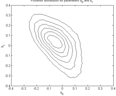
Figure 1: Posterior distribution for the parameters b₀ andb₁.

That is, our reference assumption is that the real time data on inﬂation and the output gap are equal to the lagged data on inﬂation and the output gap.

Using the Rudebusch and Svensson (1999) data set kindly provided to us by Glenn Rudebusch, we compute the errors of the RS Phillips curve,eπ

t+1,and the IS curve, eyt+1. We

then compute the errors of our reference model for the real time data on inﬂation, eπ,data_t , and the output gap ey,data_t .We model the reference models’ errors as follows:9

eπ_t₊₁ = 4 i=0 a_iLi(π_t−π_t₋₁) + 4 i=0 b_iLiy_t+ 1 + 4 i=1 c_iLi επ_t₊₁ ey_t₊₁ = 4 i=0 d_iLiy_t+ 4 i=0 f_iLi(i_t−π_t) + 1 + 4 i=1 g_iLi εy_t₊₁ eπ,data_t = 3 i=0 h_iLiπ_t+ 1 + 2 i=1 k_iLi ηπ_t ey,data_t = 3 i=0 l_iLiy_t+ 1 + 2 i=1 m_iLi ηy_t

Note that this allows for rich dynamics in the omitted variables and rich serial correlation in the shocks. An interesting extension of our analysis would be to include additional omitted variables in the model errors, reﬂecting other variables policymakers may consider.

9_{Our model for the real-time data errors has fewer lags than that for the RS model errors because our} sample of the real-time data is much shorter than our sample of the ﬁnal data

(22)

Assuming diffuse priors for all parameters, we sampled from the posterior distributions of the coefficientsa, b, c, ..., mand the posterior distributions of the shock variances using the algorithm of Chib and Greenberg (1994) based on Markov Chain Monte Carlo simulations. We obtained six thousand draws from the distribution, dropping the first thousand draws to ensure convergence. In Figure 1 we provide a contour plot of the estimate of the joint posterior density of the parametersb₀andb₁.These parameters can roughly be interpreted as measuring the error of the RS model’s estimates of the effect of the output gap on inflation. The picture demonstrates that the RS model does a fairly good job in assessing the size of the effect of a one time change in the output gap on inflation. However, there exist some chances that the effect is either more spread out over the time or, vice versa, that the initial response of inflation overshoots its long run level.

Using our sample of the posterior distribution for the parameters a, b, . . . , m we simu-lated posterior distributions of 4_t₌₀a_teitω_,4

t=0bteitω, ldots,1 +

₂

t=1mteitω on a grid over the unit circle in the complex plain. For each frequency in the grid, we found thresholds a(ω), b(ω), . . . , m(ω) such that 95% of the draws from the above posterior distribution had absolute value less than the thresholds.10 We then define weights W_a(L), W_b(L), ..., and W_m(L) as rational functions of L with numerators and denominators of fifth degree whose absolute values approximate a(ω), b(ω), ..., m(ω) well in the sense of maximizing the least squares fit on our grid in the frequency domain.

In Figure 2 we plot the thresholds b(ω), f(ω), h(ω), and l(ω) together with the absolute values of the corresponding weights. For the three out of the four reported thresholds more uncertainty is concentrated at high frequencies. However, for f(ω) which corresponds to uncertainty about eﬀect of the real interest rate on the output gap, there exists a lot of uncertainty at low frequencies.

We then tried to compute an upper bound on the worst possible loss of the Taylor rule: i_t = 1.5¯π∗_t + 0.5y_t∗

where ¯π_t∗ is a four quarter average of the real-time data on inﬂation and y∗_t is the real time data on the output gap. However this policy rule resulted in inﬁnite loss. Our description of uncertainty turns out to include some models that are unstable under the Taylor rule.

We then analyzed smaller perturbations to the reference model. We redefinea(ω), ..., m(ω) as the envelopes for the posterior distribution of uncertain gains corresponding to lower than 95% confidence level. The graph of the upper bound on the worst possible loss for the Taylor rule for different confidence levels is shown in Figure 3. We see that the worst possible loss becomes ten times higher than the loss under no uncertainty for the confidence levels as small as 1%! This roughly means that even among the 50 draws from the posterior distri-bution which are closest to zero (out of 5000 draws) we can find such parametersa, b, ..., m

10_{We deﬁne}_k₍_ω_{) and}_m₍_ω_{) as the numbers such that 95% of the draws from the posterior for 1+}2

t=1kteitω and 1 +2_t₌₁m_teitω lie closer to the posterior mean of 1 +2_t₌₁k_teitω and 1 +2_t₌₁m_teitω thank(ω) and m(ω) respectively. As Orphanides (2001) notes, the noise in real time data may be highly serially correlated. By centering the real time data uncertainty description around the posterior mean fork andm(instead of zero) we essentially improve our reference model for the real time data generating process.

(23)

Figure 2: 95% envelopes of the sampled gains of diﬀerent uncertainty channels. Dotted lines correspond to rational approximations to the envelopes.

(24)

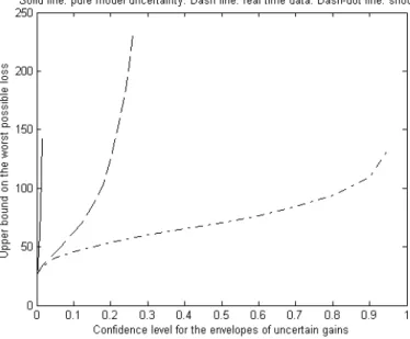
Figure 4: Upper bound on the worst possible loss. The solid line corresponds to pure model uncertainty, the dashed line corresponds to real time data uncertainty, and the dash-dot line corresponds to pure shock uncertainty.

that correspond to an economic disaster if the Taylor rule were mechanically followed by the central bank.

Recall that according to our classification, the posterior distributions for a, b, d, and f describe pure model uncertainty, the posterior distributions for c and g describe shock uncertainty, and the posterior distribution for the rest of the parameters describe real time data uncertainty. How do different kinds of uncertainty contribute to the miserable worst scenario performance of the Taylor rule? To answer this question, we increased the size of the specific uncertainty, keeping the coefficients corresponding to all other sources of uncertainty equal to the values closest to zero that were ever drawn in our simulations. The graph with contributions of different forms of uncertainty to the worst possible loss is given in Figure 4. We see that the pure model uncertainty has a huge input into the worst possible sce-nario for the Taylor rule. This result supports the common belief that under the existing amount of model uncertainty, mechanically following any Taylor-type rule specification is an extremely dangerous adventure. Alternatively, it may be indicating that policy makers have strong priors about the parameters of the true model. The pure shock uncertainty is the least important source of uncertainty. Clearly, changing the spectral characteristics of the shock process cannot make the model unstable under the Taylor rule. Even for very broad confidence regions for the spectrum of the shock processes, the worst possible loss is only about 5 times larger than the loss under no uncertainty. The real time data uncertainty significantly contributes to the worst possible scenario for the Taylor rule. It is possible to design a linear filter procedure for generating real-time data from the actual data that will mimic the historical relationship between the real time data and the final data quite well

(25)

Figure 5: Optimally robust Taylor-type rules under diﬀerent levels of prior informativeness. Labels on the graph show the worst possible losses corresponding to the robust rules. Solid line: pure model uncertainty. Dash line: pure real time data uncertainty. Dash-dot line: pure shock uncertainty.

and will lead to instability under the Taylor rule.

As we mentioned above, the poor performance of the Taylor rule under the uncertainty may be caused by our assumption of diﬀuse priors for the parameters of the true model. It may turn out that, contrary to our assumption, policy makers’ priors are very informative. To see how informativeness of the priors aﬀects the optimally robust Taylor-type rule, we do the following exercise. We start from a very informative prior which puts a lot of weight on very small values of the model error parameters. The optimally robust Taylor rule for such an extremely informative prior is essentially the optimal Taylor-type rule under no uncertainty. Then we decrease the informativeness of priors monotonically. We do this separately for the pure model, real data, and shock uncertainty parameters. We plot the corresponding optimally robust Taylor-type rules in Figure 5.

When the informativeness of the prior on the model uncertainty parameters falls, the optimally robust Taylor-type rules become less active in the inflation response and somewhat more active in the response to the output gap. This is in accordance with the results of Onatski and Stock (2002). Contrary to our expectations, when the informativeness of the prior for the real time data uncertainty falls, the optimally robust rule become more aggressive both in its response to the output and in its response to inflation. This result is caused by the fact that we allow a possibility that the real-time data on inflation is systematically underestimating the actual inflation. In such a case, an active reaction on both changes in the real-time inflation data and changes in the real-time output gap data

(26)

Figure 6: Worst possible loss for Taylor-type rules under model uncertainty only. Informative prior cali-brated so that the worst possible loss under the Taylor rule is about 80.

are needed to prevent inﬂation from permanently going out of control. Finally, the Taylor-type rules optimally robust against pure shock uncertainty are very close to the optimal Taylor-type rule under no uncertainty.

The level of the optimal worst possible loss (given on the graph) rises when the infor-mativeness of priors falls. This happens because the size of the corresponding uncertainty increases. These levels supply a potentially useful piece of information on the plausibil-ity of the corresponding prior. In our view, the levels of the worst possible loss less than about 80 correspond to plausible model uncertainty sets, and therefore to plausible priors on uncertainty parameters. Our computations show that the loss under no uncertainty for the benchmark Taylor rule is about 20. Therefore, a loss equal to 80 roughly corresponds to standard deviations for inﬂation and the output gap twice as large as those historically observed. Hence, it is not unreasonable to assume that the worst possible models implying such losses must be considered seriously by policy makers.

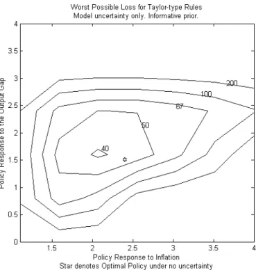
Figure 6 shows a contour plot of the worst possible losses for a broad range of the Taylor-type rules computed under an informative prior for pure model uncertainty. The level of informativeness of the prior was calibrated so that the worst possible loss under the Taylor rule was about 80. The optimally robust rule under such a prior is not very diﬀerent from the optimal policy rule under no model uncertainty (denoted by a star at the graph). The level of robustness deteriorates quickly when one deviates from the optimally robust rule. We obtained qualitatively similar results, which we do not report here, for the real time data

(27)

Uncertainty Coefficient Coefficient Worst Possible Channel on Inflation on Output Gap Loss

No uncertainty 2.4 1.5 13.1

Own dynamics of π 2.3 1.6 20.3

Eﬀect ofy on π 2.9 2.6 76.0

Own dynamics of y 2.2 2.0 29.6

Eﬀect ofr ony 2.1 1.7 146.1

News in the real-time 2.0 1.1 22.1 output gap error

Noise in the real-time 2.3 1.4 16.1 output gap error

News in the real-time 3.4 2.7 46.8 inﬂation error

Noise in the real-time 2.3 1.5 16.2 inﬂation error

Table 1: The coefficients of the robust optimal Taylor rules and corresponding worst possible losses for diffuse priors on different uncertainty channels.

uncertainty and pure shock uncertainty.

So far, we combined uncertainty about the own dynamics of inflation in the Phillips curve, uncertainty about the dynamic effect of the output gap on inflation, uncertainty about the own dynamics of the output gap in the IS curve, and uncertainty about the dynamic effect of the real interest rate on the output gap into what we called the model uncertainty. Similarly, we combined uncertainty about news and noise in the error of the real-time data on the output gap and uncertainty about news and noise in the error of the real-time data on inflation into what we called the real-time data uncertainty.11

To gain insight on the relative importance of the different blocks of model uncertainty and the real-time data uncertainty, we computed the optimally robust Taylor-type rules corresponding to a very informative (zero) prior on all channels of uncertainty except one, such as for example, uncertainty about the own dynamics of inflation in the Phillips curve. For each channel of uncertainty we consider a relatively uninformative prior so that only this specific channel matters for the robust decision maker. Our results are reported in Table 1. We see that the most dangerous block is represented by the uncertainty about the slope of the IS curve. The worst possible loss for the optimally robust rule corresponding to such uncertainty is an order of magnitude larger than the optimal loss under no uncertainty whatsoever. The least dangerous among uncertainty blocks representing model uncertainty is the uncertainty about the own dynamics of inflation. This result, however, is an artifact of

11_{Uncertainty about the coefficients}_li _{can be thought of as uncertainty about news in the error of the} real-time data on the output gap. It is because the part of the real-time data error described with the help ofl_i is correlated with the final data on the output gap. Similarly, uncertainty about the coefficientsm_i can be thought of as uncertainty about noise in the error of the real-time data on the output gap.

(28)

Uncertainty Coefficient Coefficient Worst Possible Channel on Inflation on Output Gap Loss

No uncertainty 2.4 1.5 13.1

Own dynamics of π 2.3 1.5 17.2

Eﬀect of y onπ 2.2 1.6 20.8

Own dynamics of y 2.2 1.6 20.7

Eﬀect of r ony 1.9 1.0 24.4

News in the real-time 2.1 1.2 17.8 output gap error

Noise in the real-time 2.4 1.4 15.3 output gap error

News in the real-time 2.4 1.8 21.2 inﬂation error

Noise in the real-time 2.3 1.5 15.4 inﬂation error

Table 2: The coefficients of the robust optimal Taylor rules and corresponding worst possible losses for diffuse priors on different uncertainty channels. Business cycle frequencies only.

our maintaining a vertical long-run Phillips curve. Had we allowed for a non-vertical Phillips curve in the long-run, the importance of uncertainty about the own dynamics of inﬂation would have been much higher.

Among all optimally robust rules reported in Table 1, only the rules corresponding to uncertainty about real-time data on the output gap are less aggressive than the optimal rule under no uncertainty. In fact, for the uncertainty about the coefficients l_i (which we interpret as uncertainty about news in the error of the real-time data on the output gap), the optimally robust Taylor-type rule has the coefficient on inflation 2, and the coefficient on the output gap 1.1. This is not far from the Taylor-type rule that best matches the Fed’s historical behavior (see Rudebusch (2001)). On the contrary, the optimally robust rule corresponding to the uncertainty about news in the error of the real-time data on inflation is extremely aggressive. This finding supports our explanation (given above) of the fact that the combined real-time data uncertainty implies aggressive robust policy.

We can further improve our analysis by focusing on specific frequency bands of the uncertainty. For example, we may be most interested in the uncertain effects of business cycle frequency movements in inflation and the output gap on the economy. Table 2 reports the coefficients of the optimally robust Taylor-type rules for different uncertainty blocks truncated so that the uncertainty is concentrated at frequencies corresponding to cycles with periods from 6 quarters to 32 quarters.12 In contrast to Table 1, Table 2 does not contain very aggressive robust policy rules. Now most of the robust policy rules reported are less aggressive than the optimal rule under no uncertainty. As before, the most dangerous

12_{Technically, we multiply thresholds} _a₍_ω₎_{, b}₍_ω₎_{, ..., m}₍_ω_{) by zero for frequencies outside the range} [2π/32,2π/6].