VISA: Visual Subspace Clustering Analysis
Ira Assent
Ralph Krieger
Emmanuel M ¨uller
Thomas Seidl
Data management and data exploration group, RWTH Aachen University, Germany
{assent,krieger,mueller,seidl
}@cs.rwth-aachen.de
ABSTRACT
To gain insight into today’s large data resources, data min-ing extracts interestmin-ing patterns. To generate knowledge from patterns and benefit from human cognitive abilities, meaningful visualization of patterns are crucial. Cluster-ing is a data minCluster-ing technique that aims at groupCluster-ing data to patterns based on mutual (dis-)similarity. For high di-mensional data, subspace clustering searches patterns in any subspace of the attributes as patterns are typically obscured by many irrelevant attributes in the full space. For visual analysis of subspace clusters, their comparability has to be ensured. Existing subspace clustering approaches, however, lack interactive visualization and show bias with respect to the dimensionality of subspaces.
In this work, dimensionality unbiased subspace clustering and a novel distance function for subspace clusters are pro-posed. We suggest two visualization techniques that allow users to browse the entire subspace clustering, to zoom into individual objects, and to analyze subspace cluster charac-teristics in-depth. Bracketing of different parameter settings enable users to immediately see the effect of parameters on their data and hence to choose the best clustering result for further analysis. Usage of user analysis for feedback to the subspace clustering algorithm directly improves the subspace clustering. We demonstrate our visualization tech-niques on real world data and confirm results through addi-tional accuracy measurements and comparison with existing subspace clustering algorithms.
1.
INTRODUCTION
Increasingly large data resources in life sciences, mobile in-formation and communication, e-commerce, and other appli-cation domains require computer-based techniques for gain-ing knowledge. More and more data are produced by sensor networks, technical or financial monitoring systems, scien-tific experiments, or telecommunication networks. Scien-tists developing new drugs, system administrators monitor-ing complex technical processes, and decision makers bemonitor-ing responsible for complex social or technical systems require an overview and even a deeper understanding of their mon-itored systems. Moreover, yet unknown dependencies in the observed measurements are crucial for development of new models that detect and explain causalities.
While computers efficiently support statistical and associa-tive analysis of large amounts of data, they do not reach
the high cognitive abilities of human users. Human experts are able to quickly identify both correlations and irregular-ities if data or results are appropriately visualized [13]. As “visual animals”, humans excel at expressing and analyz-ing visual entities [19]. Tasks that are inherently difficult for computers such as parametrization, or are subjective by their very nature such as redundancy or relevance to a given task, can be effectively supported by human computer in-teraction. Visualization plays a key role in interaction as it build an interface between an automated output and the human user. Visual data analysis allows to combine the ef-ficiency of computers with the cognitive strength of human users [13]. For data analysis or mining tasks, visualization is the central step from patterns to knowledge in the knowl-edge discovery process [11].
Clustering is one of the major knowledge discovery tasks. It aims at summarizing data base objects such that simi-lar objects are grouped together while dissimisimi-lar ones are separated [11]. In noisy data or data with many attributes, clusters are often hidden in subspaces of the attributes and do not show up when clustering over the full attribute space. A global reduction to relevant attributes is often infeasible, as relevance of attributes is not necessarily a globally uni-form property in the data [1; 12; 3]. Subspace clustering thus aims at identifying clusters in any possible attribute combination. As the number of possible subspace is expo-nential in the number of dimensions, this is a challenging task both with respect to efficient runtimes of the algorithm as well as to the typically enormous number of (redundant) output clusters.
For full-space clustering, different visualization techniques exist [8; 25; 9; 16; 14]. In all these approaches the same fixed set of dimensions is encoded in the visual model. These methods are thus as limited as full-space clustering: clusters are detected only if visible in the chosen mappings. As typ-ically clusters are hidden in different subspace dimensions they cannot be detected by globally defined projections and encodings.
Meaningful subspace cluster visualization requires aggrega-tion of similar results and occlusion of redundant informa-tion. Users need compact representation of different sub-space clusterings for visual analysis of relevant aspects and feedback to the algorithm. Visualization thus requires a measure of similarity for the output, as well as techniques to reduce the overwhelming number of (redundant) results common in subspace clustering. Exploiting user feedback, subspace clustering algorithms may be focused to relevant parts or subspaces of the data through explicit guidance.
In this paper, we propose a novel distance measure for sub-space clusters that reflects their inherent connections or dif-ferences, respectively. Based on subspace clustering distance models, VISA (visual subspace clustering analysis) is able to produce expressive visual diagrams that allow for meaning-ful user interaction.
For traditional full-space clustering, density-based approaches have shown to successfully mine clusters even in the pres-ence of noise [7]. The idea is to define clusters as dense areas separated by sparsely populated areas. Density-based clustering has been extended to subspace clustering in pre-vious works [12; 17]. As dimensionality is ignored in these approaches, density in subspaces of different dimensionali-ties is not comparable. Existing approaches which do not take this effect into consideration hence check incompara-ble values against the same threshold. Our density-based subspace clustering approach DUSC (dimensionality unbi-ased subspace clustering) bunbi-ased on statistical foundations takes the dimensionality into account. This method elimi-nates dimensionality bias and leads to comparable clustering results between different subspaces. This allows for mean-ingful analysis of visualized subspace clusters following our novel VISA method.
In this work, we propose visualization techniques for sub-space clustering. Our contributions include
• unbiased, comparable results based on a statistically sound subspace clustering model
• powerful yet compact visualization capable of dealing with clusters in many different projections
• meaningful ranking of the most “interesting” results to guide analysis of the output
• user interaction for parameter setting, exploration and feedback
• handling of redundant output
This paper is structured as follows: we review related work on both subspace clustering and visualization techniques in the following section. In Section 3 we formalize unbiased density-based subspace clustering. Novel visualization tech-niques for subspace clustering results, including discussion of how to rate (dis-)similarity and redundancy of the output, are presented in Section 4, before we conclude our paper.
2.
RELATED WORK
Clustering generates groups of similar objects while assign-ing dissimilar objects to different clusters [11]. In density-based clustering, clusters are dense areas separated by sparsely populated areas as in DBSCAN [7]. It has shown to be capa-ble of detecting arbitrarily shaped clusters even in noisy set-tings. Traditional clustering does not scale to high-dimensio-nal spaces. As clusters do not show across all attributes, they are hidden by irrelevant attributes [4]. Global dimen-sionality reduction techniques such as principal component analysis are typically not appropriate, as relevance is not globally uniform [5].
To detect locally relevant attributes, subspace clustering searches for clusters in any possible subset of the attributes [21]. As the number of subspaces is exponential in the number of dimensions, this is a challenging task. CLIQUE
discretizes the data using grids to reduce computational complexity, yet misses clusters which spread across several grid cells [1]. SCHISM extends CLIQUE using a variable threshold to cope with different dimensionalities, yet relies on heuristics and grid-based discretization for pruning [23]. Consequently, completeness is lost as in all grid-based ap-proaches. Specialized algorithms for categorical data or se-quences [26; 2] require discretization as well. SUBCLU ex-tends non-discretized density-based clustering to subspaces [12]. Its result, however, is biased with respect to sionality, i.e. while expected density changes with dimen-sionality, fixed density thresholds are used for pruning. Visual data analysis techniques benefit from human cogni-tive abilities in data mining through user interaction. For traditional clustering in general, various visualization tech-niques have been proposed [8; 25; 9; 16; 14]. In all these cases, the same dimensions of the data space are encoded by the same projections or parameters in the visual model. The methods thus behave as limited as full-space clustering does: Clusters are only detected if they are visible in the re-spective chosen mappings. As typically clusters are hidden in different subspace dimensions they cannot be detected by globally defined projections and encodings.
Additionally, subspace clustering visualization has to deal with the exponential number of subspace projections and the typically enormous redundancy of the result. As different projections contain different clusters, visualization should provide an overall overview as well as means for in-depth analysis and interaction. Special cases like mosaic encodings in gene-expression analysis [6] order clusters by biological properties like position of a gene on the chromosomes. This underlying ordering does not extend to other application do-mains. As there is no inherent ordering in general subspace clustering applications, lack of (dis-)similarity measures and poor comparability of results are major hindrances for visu-alization.
3.
SUBSPACE CLUSTERING
Our VISA (visual subspace clustering analysis) approach vi-sualizes subspace clustering for user interaction. As men-tioned above, this requires comparable clustering results in any subspace. Existing subspace clustering approaches do not take changing expected density values for different di-mensionalities into account. Consequently, these approaches suffer from an effect we calldimensionality biasthat hinders meaningful comparison of results.
We formalize density estimation and our notion of dimen-sionality bias, before proposing an unbiased density estima-tor that leads to comparable subspace clustering results. LetU= [0,v] be a universal domain for all dimensions,D=
{1, . . . , d}be an index set, andDB⊆UD a d-dimensional data base with n objects. A subspace US is the projec-tion of UD to ther dimensions specified by the index set S = {s1, . . . , sr} ⊆D. Analogously, letDBD denote the
original data base and DBS its projection to the dimen-sions inS. For ease of notation, we refer to a subspaceUS
by its index setS. The definition of density-based subspace clusters extends standard notions in density-based clustering [7]. Let k.kS
denote the restriction of normk.k:UD → R
to the dimensions in subspace S. The area of influence is the neighborhood in subspaceS:
NS
an objectois determined by simply counting the number of objects in a fixedε-rangeNS
ε(o). We generalize this idea by
assigning weights to each object contained inNS
ε(o).
Definition 1. Density Measure
Let W be an arbitrary weighting function W : R → R. Based on W, a generalized density measure ϕS(o) for an objectoin subspace Sis defined as:
ϕS(o) = X
p∈NS
ε(o)
Wko−pkS
Thus, an objectoin subspaceSis calleddenseif the weighted distances to objects in its area of influence sum up to more than a given density thresholdϕS(o)≥τ.
3.1
Dimensionality Bias
Incomparable density values pose the following problem: the high discrepancy in density scales of low-dimensional or high-dimensional subspaces makes it impossible to find a suitable parameter for a fixed density thresholdτ. If on the one handτ is parametrized such that high-dimensional clusters with low expected density are detected then numer-ous excess pseudo-clusters are generated in low-dimensional spaces where expected density is high. On the other hand, a parametrization ofτ which separates clusters from noise in low-dimensional spaces loses clusters in high-dimensional spaces. We assume thatτ is fixed as dimensionality depen-dent thresholds can also be incorporated into the density measure.
To obtain comparable density values, unbiased density mea-sures have to be independent of the dimensionality of the subspace. Statistically speaking, this corresponds to the same expected density value regardless of the dimensionality of the subspace.
Definition 2. Dimensionality Unbiased Density Mea-sure
A density measureϕS is dimensionality unbiased if its
ex-pected density is the same for any two subspaces S1 and
S2⊆D:
∀S1,S2: EhϕS1i=EhϕS2i
We now show how dimensionality bias can be eliminated for any density estimator. As the expected density should be the same for any two subspaces, we normalize density esti-mators with their expected density. For any density measure
ϕS, the normalized measure 1
E[ϕS]ϕ S
is dimensionality un-biased. With linearity property of the expectation, this is straightforward: E[E[1ϕS]ϕ
S
] = E[1ϕS]E[ϕ S
] = 1 for all sub-spaces. Thus, for any two subspaces, normalizing the den-sity measure by the expected value of the subspace yields comparable density values for any two subspacesS1andS2. Comparable density values yields consistent results. This is important both for the mining process as well as for visual-izing coherent views.
The computation of an unbiased density measure is given in [3] for the Epanechnikov kernel as density measure [24]. Similarly, normalization of any other density measure with respect to dimensionality can be performed.
3.2
The unbiased DUSC approach
Intuitive density threshold. The density threshold is a core parameter since it sets the dividing line between dense objects and noise. As this parameter has to be set by the user it is important for users to have an intuitive under-standing of this parameter. Commonly, users do not know density distribution apriori, which makes the choice of a den-sity value difficult. We exploit the fact that in our approach density is measured with respect to the expected density as discussed before. Consequently, users do not need to specify absolute density thresholds, but only a factor by which the expected density has to be exceeded. Following the defini-tion in the previous secdefini-tion, an objectois dense in subspace
Saccording to the expected densityα(S) iff: 1
α(S)ϕ
S
(o)≥F
whereFdenotes the density threshold. As the density factor
Fis independent of the dimensionality and data set size, it is much easier to specify and its setting can additionally be supported by an overall visualization of the clustering result.
Empty space problem. With increasing dimensionality the expected density and hence the expected number of objects contained in an area of influence drops exponentially [4]. This effect is termed “empty space problem” in statistics [24]. Compared to the expected density, an object may be determined as dense even if the area of influence is nearly devoid of observations, resulting in pseudo-dense single ob-jects. To remove pseudo-dense objects, we introduce a spe-cific density constraint on the expected density ofηobjects in the area of influence. The expected density value of an object o which contains η objects in the area of influence
Eη h
1
α(S)ϕ S
(o)ican be computed from the expected density of the density measure. Details for the Epanechnikov kernel can be found in [3].
To guarantee that objects are not considered dense if theε
sphere is virtually empty, a very small value for η is suffi-cient (generally two or three). Users typically do not need to change this value. Our new density-based subspace clus-tering model below combines the density constraintsαand
ω[3]. αandωcombined ensure an unbiased density notion without defining objects in nearly empty regions as dense.
Redundancy. Since the number of possible subspace pro-jections is exponential in the number of dimensions, sub-space clustering algorithms often produce numerous redun-dant subspace clusters. To avoid excessive cluster outputs which contain essentially the same information repeated in different dimensionalities, we check if a clusterCin subspace
Sis redundant. We define a cluster as redundant if (most of) the objects contained in the cluster are also contained in another cluster in a higher dimensional subspaceS0⊃S. We use a parameter Rto specify the degree of redundancy acceptable to the user. To restrict the output to a reason-able size a strict redundancy parameter is often appropriate and can be chosen from suitable visual representations. So far, we have studied the density of individual objects. Subspace clusters, following density-based clustering paradigm, are connected sets of dense objects. To ensure that clusters reflect the inherent structure of the data, they should con-tain a cercon-tain minimum number of objects. This constraint
minSizeis typically about 1% of the data base size. The resulting subspace cluster model taking these
conclu-Figure 1: Subspace clustering overview: the diameter de-picts the number of objects in the cluster, the color denotes the dimensionality (the darker, the more dimensions)
sions into account is formalized in the following.
Definition 3. DUSC Subspace Cluster
A set of objectsC ⊆DBin subspaceS⊆D is a subspace cluster if:
• objects inC areS-connected:
∀o, p∈C: ∃k: ∀i= 1, . . . , k−1 : ∃qi∈C:
kqi−qi+1kS≤ε∧q1=o, qk=p
• more dense than expected and not pseudo-dense:
∀o∈C: ϕS(o)≥max{F·α(S), η·ω(S)}
• C ismaximal, i.e. contains allS-connected objects
∀o, p∈DB,o, pS-connected⇒(o∈C⇔p∈C)
• minimum cluster size: |C| ≥minSize • not redundant: ¬∃(C0,S0)subspace cluster with
C0⊆C∧S⊂S0∧ |C0| ≥ R · |C|
The DUSC subspace clustering model extends existing density-based notions of maximality and connectedness with statis-tically sound density computation via normalized Epanech-nikov kernel and expected density. Clusters contain a sig-nificant part of the data, and are not redundant.
Evaluating the cluster model for all possible subspaces is in-feasible as their number is exponential with respect to the dimensionality. In our subspace clustering algorithm we thus avoid excess subspace cluster evaluation through (1) a filter-and-refine architecture using the weakest density threshold of all subspaces as filter pruning, (2) a depth first compu-tation on a specialized index structure, and (3) redundancy pruning.
4.
VISA
The DUSC algorithm from the previous section is used to mine subspace clusters. The resulting patterns have to be
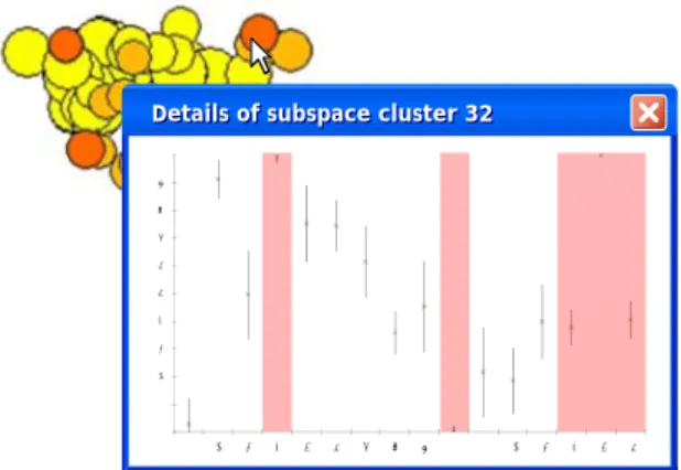
Details of subspace cluster 32
Details of subspace cluster 32
0 10 20 30 40 50 60 70 80 90 100 1 2 3 4 5 6 7 8 9 10 11 12 13 14 15 16
Figure 2: Detailed view for one subspace cluster: mean and variance for each dimension of the subspace cluster
analyzed by users for knowledge generation. This analysis is still challenging as there are many different subspace projec-tions and possibly redundant subspace clusters. We define the set of subspace clusters that have to be analyzed:
Definition 4. Subspace Clustering
A subspace clustering is a set of clusters in their correspond-ing subspaces {(C1,S1), . . . ,(Cn,Sn)}, where Ci is a
sub-space cluster in subsub-spaceSi as specified in Definition 3.
For user benefit, it is necessary to visualize subspace clus-terings such that the entire output can be browsed even for clusters in different subspace projections, and that detailed views into individual subspace clusters are possible. More-over, feedback for subsequent guiding of subspace clustering runs should be provided. This requires visual support for analysis of parameter settings as well as a focus on the most “interesting” results.
We therefore define a set of criteria that should be included in visualization:
Definition 5. Visual analysis criteria
A subspace clustering visualization should represent the fol-lowing subspace clustering properties:
• space overlap, i.e. the number of common subspaces for any two cluster subspacesSiandSj: S =|Si∩Sj|
• object overlap, i.e. the number of common objects in any two subspace clustersCi andCj: O=|Ci∩Cj|
• interestingness, i.e. the factor I by which the ex-pected density is exceeded on average for any subspace clusterCi in subspaceSi: I(Ci,Si) = P o∈Ciϕ Si(o) |Ci| ·α(Si)
The above aspects are crucial for our VISA approach, since they are necessary for in-depth analysis of subspace cluster-ings, where large result sizes easily occlude the most inter-esting, novel patterns. Next, we show how compact repre-sentation and detail information on subspace clusters can be combined for browsing. After this, we focus on bracketing and in-depth analysis.
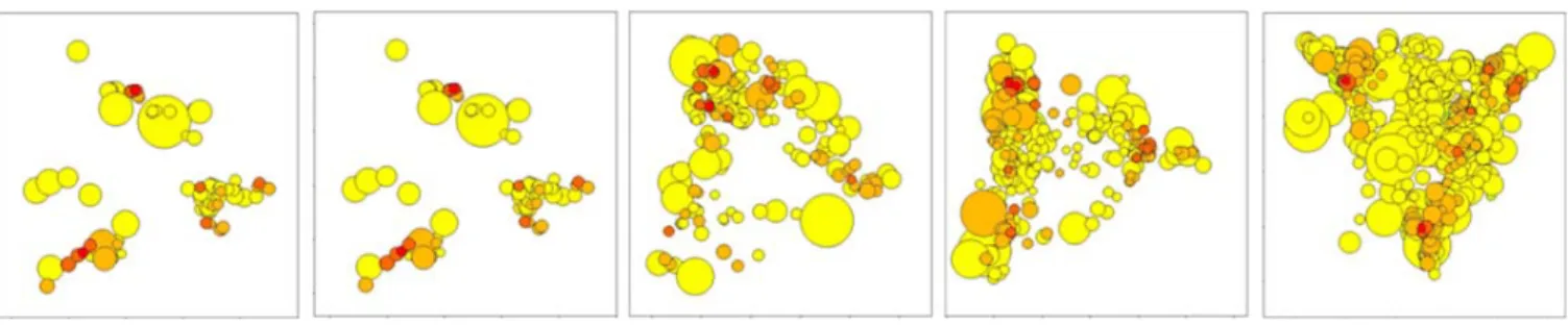
Figure 3: Bracketing Redundancy in MDS images (from left to rightR= 0%,2%,5%,7%,10%): for each parameter setting, the output is illustrated, allowing users to pick appropriate settings from the series of images easily
4.1
Browsing subspace clusterings
To give a general overview over the entire subspace cluster-ing, basic structural information of subspace clusters should be compactly represented. Interactively, details should be provided for individual clusters during browsing.
The major challenge for any overview visualization of sub-space clusterings lies in the comparability of subsub-space clus-ters. As subspace clustering algorithms may identify pat-terns in completely different or overlapping subspaces, we have to define (dis-)similarity of subspace clusters on a gen-eral scale. We propose a distance function for comparing any two subspace clusters that takes both the subspace overlap and the object overlap into account. It is defined as a con-vex sum of the difference in subspaces and the difference in cluster objects:
Definition 6. Subspace Cluster Distance
The distance between two subspace clusters Ci,Cj in
sub-spacesSi,Sj, respectively, is defined as the convex sum of
subspace distance and object distance:
β 1−|Si∩Sj| |Si∪Sj| + (1−β) 1− |Ci∩Cj| min{|Ci|,|Cj|}
This distance function thus allows comparing subspace clus-ters for a general overview. Independent of any application specific properties of the data, similarity can be measured by incorporating the criteria presented in Definition 5. Normalization of both subspace and object distance is to a range of zero to one, respectively. We use two different normalizations for object and subspace distances.
1.) Object distance: a fully redundant subspace cluster is a lower dimensional projection of an interesting subspace clus-ter (object overlap). For visualization, inclus-teresting subspace clusters should be stacked upon their redundant counter-parts, i.e. the distance should be zero. This is achieved by normalizing object distance by minimum cluster size. For redundant subspace clusters, the minimum in the denomi-nator is the same as the intersection in the numerator, and object distance is indeed zero.
2.) For subspace distances, clusters in subsets of dimensions may very well differ in all objects. They share subspace projections, yet do not actually overlap. Their subspace distance should therefore still reflect the difference in the remaining dimensions, and not be zero. To this end, nor-malization is by the union of subspaces. For visualization, this means that sub-projections are located close to each other.
Object overlap can be further favored by choosingβsmaller than 0.5 to give more weight to object distance.
An overview over the distances of all subspace clusters can be achieved by multidimensional scaling (MDS) [18]. Simply put, it allows for nonlinear projection of objects from their original distance space to a 2D or 3D visualization space, preserving mutual distances as much as possible. In our MDS image of the subspace clustering result, the distance information is enriched by information on the size and the dimensionality of a subspace clusters. For a general overview size and dimensionality of subspace clusters can be visual-ized by the radius of the circles and their color, respectively (see Figure 1). Consequently, browsing the entire output is possible. However, this enriched MDS image by itself does not provide sufficient information for user analysis. To get a better understanding of why subspace clusters are similar or different and for browsing the actual objects in subspace clusters, detailed information should be available upon click on subspace cluster representations. As individual objects in subspace clusters are typically more than two-dimensional, we represent the distribution of objects in a subspace cluster by a mean and variance plot for all dimensions. Addition-ally, we highlight those dimensions that are relevant for the subspace cluster (see Figure 2).
4.2
Bracketing
Bracketing refers to a technique originally from photogra-phy. Several different camera settings are used to take a series of pictures of the same subject. Photographers then pick the best setting among the resulting pictures. It has been discussed in human computer interaction in [22]. We propose bracketing for subspace clustering visualization as a useful technique that demonstrates the effects of parametriza-tion. It provides not just a single subspace clustering output, but a series to choose from. This allows users to analyze the effect of different parameters at a single view.
As we have seen already in Figure 1, the clustering shows groups of subspace clusters. In their center we have the desired high-dimensional (red) subspace clusters containing few objects (small circle). These high-dimensional clusters in lower projections again form clusters, which are depicted as large yellow circles. This effect can be reduced by our redundancy parameter R, as we can see in Figure 3. The overwhelming result forR = 10%, i.e. redundancy of 10% is permitted, gives us evidence of poor cluster quality as in large low-dimensional clusters not only hidden clusters are found but also noise. As we will see later in accuracy anal-ysis, removing such redundant clusters leads to a significant quality improvement of the overall clustering result.
G2
G3
Dimension
G1
2 3 4 5 6 7 8 9 10
Figure 4: Matrix of subspace clusters groups. Rows represent the cluster and columns the dimensions, groups are separated by white lines (see right part). Color map HSV: hues represent the value in each dimension of the subspace cluster; saturation and value represent the factorIof interestingness.
4.3
In-depth analysis
As illustrated in Section 4.1, subspace clusterings visualized in MDS images typically form groups of similar subspace clusters. For in-depth analysis, visualizing characteristics of each of these groups of subspace clusters in a compact way is important. Characteristics are joint and distinct properties of groups of subspace clusters. Properties of importance are the interestingness I of a subspace cluster as well as the subspace and object overlap. Visualizing these properties is necessary for in-depth analysis of the overall subspace clustering.
Subspace clusters are grouped if they share dimensions or if they have objects in common, as defined by our subspace cluster distance function. To visualize these groupings such that similarities show up as clear visual patterns, we pro-pose to plot all groups of subspace clusters and the objects contained in each group. Each group is defined as the set of all subspace clusters similar to a subspace cluster of high interest (see Def. 5). We call the most interesting subspace cluster of a group theanchor of the group. Agroup is then defined as all subspace clusters of at mostϑdistance to the anchor.
To visualize a group of subspace clusters we use a matrix representation. We start with the subspace cluster having the highest interest. Hence this cluster is the anchor of the first group. Starting with the anchor each subspace clus-ter of a group is represented by its objects. Each object is depicted by one row whereas the columns illustrate the dimensions of the object. To allow an in-depth analysis we use different color codes to visualize all characteristics of an object, that is its interestingness as well as the values in each dimension. If a dimension is not part of a cluster the column is black.
To highlight subspace clusters of high interestingness we use the factorIas saturation and value in HSV color space [10]. Hence interesting subspace clusters can be easily identified
as the active dimensions are represented by bright and in-tensive colors. To represent the value for each dimension we use the hue value according to the HSV space. By using all possible hue values the complete color range is used to encode the value of an object but other mappings can be used as well. Further on, objects are ordered with descend-ing interest. Redundant objects that are already visualized
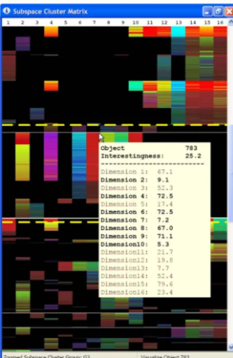
Figure 5: User Interface for a Subspace Clusters Matrix: By pointing on individual objects additional information about the cluster is visualized
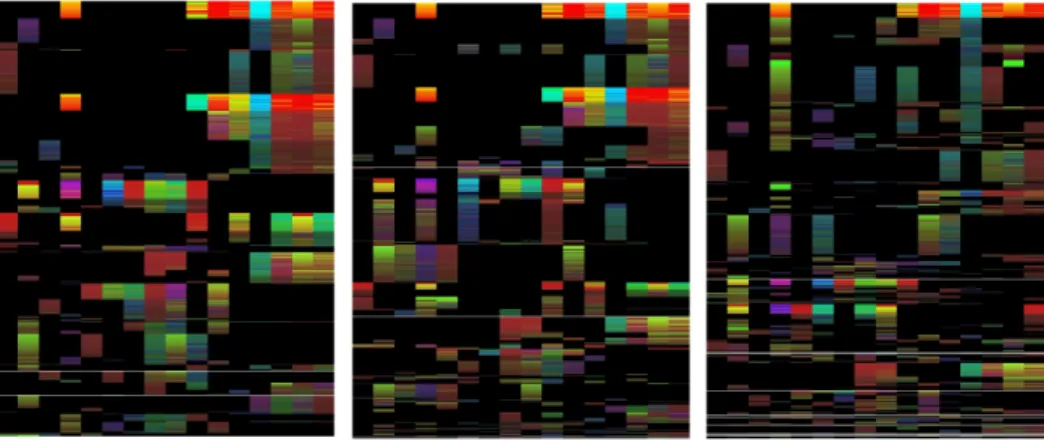
Figure 6: Bracketing Matrix forR= 0%,5%,10%: for each parameter setting, the output is illustrated, allowing users to pick appropriate settings from the series of images easily
in other clusters are omitted in order to obtain a compact and descriptive representation of the complete clustering. Once all objects of a subspace cluster have been presented the next subspace cluster with respect to the next anchor is displayed.
Figure 4 illustrates the subspace cluster groups for the Pendig-its data set usingR= 0%. As discussed, a group of subspace clusters typically has some dimensions in common (thecore dimension of a group). Our proposed subspace clustering matrix allows for visual recognition of core dimensions. Con-sider the groupG3 zoomed in on the right side of Figure 4, dimensions 2, 4 and 6 to 10 can be easily identified as core dimensions. By comparing the different groups illustrated in Figure 4 we can see that many subspace clusters identi-fied correlations in dimension 12 to 16 (e.g. G1,G2, etc.), while some other groups also have a core containing the di-mensions 6 to 10 (e.g.G3). Further on, a density connected fullspace cluster (a cluster considering all dimensions) is not found (no completely colored row contained in Figure 4). Additionally, detailed information about an object can be obtained by moving the mouse over the object. Figure 5 illustrates a user interface for visualizing a subspace clus-ter matrix. Information about the inclus-tersestingness and the values of an object can be presented in a tool tip. Hence, details about thecenter of a group(i.e. the objects of high-est interhigh-est) can be easily obtained by the user by moving the mouse over the first objects of a group. For precise se-lection of individual objects the scroll bar can be used for an interactive zoom of specific areas of the subspace cluster-ing matrix (illustrated in Figure 5 by the area surrounded by the yellow lines). The area above and below the yellow lines shows the original compact representation as depicted in Figure 4. In-between the lines, rows are enlarged by a specified factor. Scrolling up or down, the zoom area can be varied.
Bracketing as shown in Figure 6 illustrates the subspace cluster groups for different redundancy setting (left part
R = 0%, middleR = 5% and right part R = 10%). As can be easily seen, a clear clustering structure is obtained if redundancy is removed (leftmost matrix). Small subspace groups are removed if less redundancy is allowed. Hence, re-moving redundancy improves the clustering structure. We validate this visual impression of improved quality by addi-tional measurements on the accuracy and quality of DUSC,
comparing it to two recent subspace clustering algorithms, SUBCLU [12] and SCHISM [23]. In addition to the previ-ously used Pendigits data, we used Glass and Vowel from [20] and Shapes from [15]. Quality is determined using the entropy, i.e. H(C) =−Pk
i=1p(i|C)·log(p(i|C)) forkclass
labels in clusterC. For a set of clusters we take the average entropy weighted by the number of objects per cluster. For readability, inverse entropy is normalized to a range of 0% to 100%.Coverage (C) is the percentage of objects in any subspace cluster. It indicates the ratio of clustered objects to noise. The amount of noise in a data set is typically not known apriori, but noise is present in most real world data sets. As sparsely populated regions often exhibit a weak cor-relation to the class label, quality may increase if coverage decreases.
The first column in Figure 7 shows the best quality (Q) re-sults of DUSC with R = 0% as also seen from bracketing redundancy. Allowing more redundancy, coverage increases and quality goes down slightly. However, even forR= 10% DUSC shows better quality than the competing algorithms. The fact that coverage is not 100% indicates that DUSC can distinguish between noise and clusters in subspaces of varying dimensionalities as also illustrated by Figure 6. The pendigits data set, for example, contains handwritten num-bers, some of which are clearly different from the rest of the data set. Biased algorithms like SCHISM and SUBCLU do not detect noise, but assign all objects to clusters. The last data set SHAPE contains rotated versions of 9 different shapes, but only 3 of the shapes clearly form clusters. Thus most of the objects have to be considered noise. DUSC de-tects the given clusters correctly while SCHISM dede-tects only a small part of the clusters and SUBCLU mixes up clusters with noise (less than 100% quality).
DUSC 0% DUSC 5% DUSC 10% SUBCLU SCHISM
Q C Q C Q C Q C Q C
Pendigits 86 74 83 87 81 92 58 100 77 100
Glass 60 87 51 90 50 93 44 100 44 99
Vowel 82 70 79 100 74 100 10 100 42 100
Shape 100 31 100 31 100 31 98 82 100 1
Thus the visual impression of our subspace clustering visu-alizations (see Figure 6) can be confirmed by these measure-ments.
5.
CONCLUSION
We introduced the first subspace clustering visualization to the best of our knowledge. Based on comparable results, i.e. unbiased subspace clustering, browsing of the result is possible through a novel distance function that reflects the subspace and the object overlap, respectively. Subspace clustering interestingness is incorporated to show the most relevant results. Interaction is possible through zooming in to objects in subspace clusters and through choice of ade-quate subspace clustering settings and feedback.
6.
REFERENCES
[1] R. Agrawal, J. Gehrke, D. Gunopulos, and P. Ragha-van. Automatic subspace clustering of high dimensional data for data mining applications. InProc. ACM Intl. Conf. on Management of Data, pages 94–105, Seattle, Washington,USA, June 2-4 1998.
[2] I. Assent, R. Krieger, B. Glavic, and T. Seidl. Spa-tial multidimensional sequence clustering. InProc. 6th IEEE Intl. Conf. on Data Mining - Workshops, pages 343–348, 2006.
[3] I. Assent, R. Krieger, E. M¨uller, and T. Seidl. Dusc: Dimensionality unbiased subspace clustering. In Proc. IEEE Intl. Conf. on Data Mining, Omaha, Nebraska, USA, 2007.
[4] K. Beyer, J. Goldstein, R. Ramakrishnan, and U. Shaft. When is nearest neighbors meaningful. In Proc. 7th Intl. Conf. on Database Theory, pages 217–235, Jerusalem,Israel, 1999.
[5] R. Duda, P. Hart, and D. Stork.Pattern Classification. Wiley, New York, 2001.
[6] M. Eisen, P. Spellman, P. Brown, and D. Botstein. Cluster analysis and display of genome-wide expression patterns. InProc. National Academy of Science of the USA, volume 95, pages 14863–14868, 1998.
[7] M. Ester, H. Kriegel, J. Sander, and X. Xu. A density-based algorithm for discovering clusters in large spa-tial databases. InProc. 2nd Intl. Conf. on Knowledge Discovery and Data Mining, pages 226–231, Portland, Oregon, USA, 1996.
[8] U. Fayyad, G. G. Grinstein, and A. Wierse, editors. Information visualization in data mining and knowl-edge discovery. Morgan Kaufmann Publishers Inc., San Francisco, CA, USA, 2002.
[9] M. Ferreira de Oliveira and H. Levkowitz. From visual data exploration to visual data mining: a survey.IEEE Transactions on Visualization and Computer Graphics, 9(3):378–394, 2003.
[10] J. D. Foley, A. van Dam, S. K. Feiner, and J. F. Hughes.Computer Graphics (2nd ed. in C): Principles and Practice. Addison-Wesley, Boston, MA, USA, 1996.
[11] J. Han and M. Kamber. Data Mining: Concepts and Techniques. Morgan Kaufmann, San Francisco, CA, USA, 2001.
[12] K. Kailing, Kriegel, H.-P., and P. Kr¨oger. Density-connected subspace clustering for high-dimensional data. In Proc. 4th SIAM Intl. Conf. on Data Mining, pages 246–257, 2004.
[13] D. Keim. Information visualization and visual data minig.IEEE Transactions on Visualization and Com-puter Graphics, 8:1–8, 2002.
[14] D. A. Keim, F. Mansmann, J. Schneidewind, and H. Ziegler. Challenges in visual data analysis. InProc. IEEE Intl. Conf. on Information Visualization, pages 9–16, 2006.
[15] E. Keogh, L. Wei, X. Xi, S.-H. Lee, and M. Vlachos. LB Keogh supports exact indexing of shapes under ro-tation invariance with arbitrary represenro-tations and distance measures. In Proc. 32nd Intl. Conf. on Very Large Data Bases, pages 882–893, 2006.
[16] B. Kovalerchuk and J. Schwing. Visual and Spatial Analysis - Advances in Data Mining, Reasoning, and Problem Solving. Springer, 2004.
[17] H.-P. Kriegel, P. Kr¨oger, M. Renz, and S. Wurst. A generic framework for efficient subspace clustering of high-dimensional data. InProc. 5th IEEE Intl. Conf. on Data Mining, pages 250–257. IEEE Computer Society, 2005.
[18] J. B. Kruskal. Multidimensional scaling by optimizing goodness of fit to a nonmetric hypothesis. In Psychome-trika, volume 29, pages 1–27. Springer New York, 1964. [19] M. Lucente. Diffraction-Specific Fringe Computation for Electro-Holography. PhD thesis, Massachusetts In-stitute of Technology, 1994.
[20] D. Newman, S. Hettich, C. Blake, and C. Merz. UCI repository of machine learning databases, 2006. [21] L. Parsons, E. Haque, and H. Liu. Subspace clustering
for high dimensional data: a review. ACM SIGKDD Exploration Newsletter, 6(1):90–105, June 2004. [22] J. C. Roberts. Exploratory visualization using
bracket-ing. In Proc. ACM Working Conference on Advanced Visual Interfaces, pages 188–192, New York, NY, USA, 2004. ACM.
[23] K. Sequeira and M. Zaki. SCHISM: A new approach for interesting subspace mining. In Proc. 4th IEEE Intl. Conf. on Data Mining, pages 186–193, Washington, DC, USA, 2004. IEEE Computer Society.
[24] B. Silverman. Density Estimation for Statistics and Data Analysis. Chapman and Hall, London, 1986. [25] T. Soukup and I. Davidson.Visual Data Mining:
Tech-niques and Tools for Data Visualization and Mining. Wiley, 2002.
[26] M. Zaki, M. Peters, I. Assent, and T. Seidl. CLICKS: An effective algorithm for mining subspace clusters in categorical datasets.Data and Knowledge Engineering, 60:51–70, January 2007.