On Expressiveness and Uncertainty Awareness in
Rule-based Classification for Data Streams
Thien Lea, Frederic Stahla, Mohamed Medhat Gaberb, Jo˜ao B´artolo Gomesc, Giuseppe Di Fattaa
aUniversity of Reading, Department of Computer Science, University of Reading,
Whiteknights, Reading, Berkshire RG6 6AY, United Kingdom
bSchool of Computing and Digital Technology, Birmingham City University, Curzon St,
Birmingham B4 7XG, England, United Kingdom cDataRobot, Inc.
Abstract
Mining data streams is a core element of Big Data Analytics. It represents the velocity of large datasets, which is one of the four aspects of Big Data, the other three being volume,variety andveracity. As data streams in, mod-els are constructed using data mining techniques tailored towards continuous and fast model update. The Hoeffding Inequality has been among the most successful approaches in learning theory for data streams. In this context, it is typically used to provide a statistical bound for the number of examples needed in each step of an incremental learning process. It has been applied to both classification and clustering problems. Despite the success of the Hoeffding Tree classifier and other data stream mining methods, such mod-els fall short of explaining how their results (i.e. classifications) are reached (black boxing). The expressiveness of decision models in data streams is an area of research that has attracted less attention, despite its paramount of practical importance. In this paper, we address this issue, adoptingHoeffding Inequality as an upper bound to build decision rules which can help decision makers with informed predictions (white boxing). We termed our novel method Hoeffding Rules with respect to the use of the Hoeffding Inequality
in the method, for estimating whether an induced rule from a smaller sample
Email addresses: [email protected](Thien Le),
[email protected] (Frederic Stahl),[email protected] (Mohamed Medhat Gaber),[email protected](Jo˜ao B´artolo Gomes),
would be of the same quality as a rule induced from a larger sample. The new method brings in a number of novel contributions including handling uncer-tainty through abstaining, dealing with continuous data through Gaussian statistical modelling, and an experimentally proven fast algorithm. We con-ducted a thorough experimental study using benchmark datasets, showing the efficiency and expressiveness of the proposed technique when compared with the state-of-the-art.
Keywords:
Data Stream mining, Big Data Analytics, Classification, Expressiveness, Abstaining, Modular Classification Rule Induction
1. Introduction
One problem the research area of ‘Big Data Analytics’ is concerned with is the analysis of high velocity data, also known as streaming data [1, 2], that challenge our computational resources. The analysis of these fast streaming data in real-time is also known as the emerging area of Data Stream Mining (DSM) [2, 3]. One important data mining technique, and in turn DSM category of techniques is classification. Traditional data mining builds its classification models on static batch training sets allowing several iterations over the data. This is different in DSM as the classification model needs to be induced in a linear or sublinear time complexity [4]. Furthermore, DSM
10
classification techniques need to allow dynamic adaptation to concept drifts as the data streams in [4]. Applications of DSM classification techniques are manifold and comprise for example monitoring the stock market from handheld devices [5], time monitoring of a fleet of vehicles [6], real-time sensing of data in the chemical process industry using soft-sensors [7], sentiment analysis using real-time micro-bogging data such as twitter data [8], to mention a few.
The challenge of data stream classification lies in the need of the classifier to adapt in real-time to concept drifts, which is significantly more challeng-ing if the data stream is of high velocity. Many data stream classification
20
this could be a disadvantage for real-time applications.
The here presented work proposes theHoeffding Rules data stream clas-sifier that is based on modular classification rules instead of trees. Hoeffding Rules can easily be assimilated by humans, and at the same time does not require unnecessary information to be available for the classification tasks.
30
Rule induction from data streams can be traced back to theVery Fast Deci-sion Rules (VFDR) [13] and eRules data stream classifiers [9] for numerical data. eRules induces modular classification rules from data streams, but re-quires extensive parameter tuning by the user in order to achieve adequate classification accuracy including the setting of the window size. Noting this drawback that affects the accuracy, if the parameters are not set correctly, a statistical measure that automatically tunes the parameters is desirable. Addressing this issue, Hoeffding Rules adjusts these parameters dynamically with very little input required by the user. The here presented Hoeffding Rules algorithm is based on the Prism [12] rule induction approach using a
40
sliding window [14, 15]. However, this window for buffering training data is adjusted dynamically by making use of the Hoeffding Inequality [16]. One important property of Hoeffding Rules compared with the popular Hoeffding Tree data stream classification approach [10] is, that Hoeffding Rules can be configured to abstain from classifying an unseen data instance when it is uncertain about its class label. In addition, our approach is computation-ally efficient and hence is suitable for real-time requirements. An important strength of the proposed technique is the high expressiveness of the rules. Thus, having the rules as the representation of the output can help users in making timely and informed decisions. Output expressiveness increases
50
trust in data stream analytics which is one of the challenges facing adaptive learning systems [17]. To address the expressiveness issue for offline black box machine learning models, the new algorithm Local Interpretable Model-Agnostic Explanations (LIME) has been proposed in [18]. The method gen-erates a short explanation for each new classified or regressed instance out of a predictive model, in a form that is interpretable by humans (can be expressed as rules, in a way). The work has attracted a great deal of media attention, and has emphasised the need for expressive models. Model trust has been further emphasised. This work and many other follow-up research papers have been the result of experimental work that showed some serious
60
obvious examples to humans. Again, model interpretability and trust have been emphasised as an important area of research.
The utility of expressiveness is introduced in this paper to refer to the cost of expressiveness when comparing the accuracy of two methods. As ac-curacy has been the dominating measure of interest in comparing classifiers in both static and streaming environments, it is evident that real-time deci-sion making based on streaming models still suffers from the issue of trust
70
[17]. To address this issue, the user is able to determine an accuracy loss band (ζ), such that the model can be expressive enough to grant trust, and at the same time the accuracy can be tolerated at (−ζ%) of any other best performing classifier which is less expressive (can be a total black box). We argue that such a new measure will open the door for more trustful white box models. In many applications (e.g., surveillance, medical diagnosis, terrorism detection), decisions need to be based on clear arguments. In such applica-tions, having a trustful model with a competent accuracy can be much more appreciated than having a highly accurate model that does not convey any reasoning about its decision. Other examples of applications that require
80
convincing arguments can be found in [18].
This paper is organised as follows: Section 2 highlights works related to the Hoeffding Rules approach. Section 3 highlights our dynamic rule induc-tion and adaptainduc-tion approach for data streams. An experimental evaluainduc-tion and discussion is presented in Section 4. Concluding remarks are provided in Section 5.
2. Related Work
The velocity aspect of the Big Data trend is the main driver of work done for over a decade in the area of data stream mining - long before the Big Data term was coined. Among the proposed techniques in the area come a long
90
list of classification techniques. Approaches to data stream classification varied from approximation to ensemble learning. Two motives stimulated such developments: (1) fast model construction addressing the high speed nature of data streams; and (2) change in the underlying distribution of the data, in what has been commonly known as concept drift.
the sum of a random variable deviates from its expected value. The basic
100
Hoeffding bound has been extended and adopted in successfully developing a number of streaming techniques that were termed collectively as Very Fast Machine Learning (VFML) [20].
Earlier work on data stream mining addressed the aforementioned issues. However, the end user perspective has been greatly missing, and hence the user’s trust in such systems was frequently questioned. This issue has been discussed in a position paper by Zliobaite et al [17].
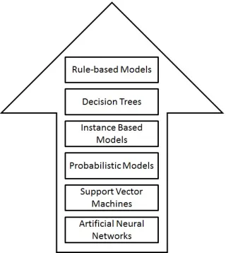
Figure 1: Hierarchy of Output Expressiveness.
In this paper we address this issue, attempting to provide the end user with the most expressive knowledge representation for data stream classifica-tion, i.e., rules. We argue that rules can provide the users with informative
110
decisions that enhance the trust in streaming systems. Figure 1 shows a hierarchy of output expressiveness, with rule-based models being at the top of all of the other classification techniques.
2.1. Rule Induction from Data Streams
FLORA is a family of algorithms for data stream rule induction that adjusts its window size dynamically using a heuristic based on the predic-tive accuracy and concept descriptions. The most recent FLORA algorithm, FLORA4, addresses the issue of concept drift. It can use previous concept descriptions in situations of recurring changes and is robust to noise in the data stream [21]. From the AQ-PM family of algorithms, the AQ11-PM
system is the most representative. AQ11-PM uses learned rules to select data instances from the training data that lie on the boundaries of induced concept descriptions and is storing these so-called ‘extreme ones’ in partial memory [22]. However, those approaches are still not adapted to high speed data stream environments, especially those featuring continuous attributes. The FACIL [23] algorithm works similarly to AQ11-PM. However, FACIL does not require all stored data instances to be extreme and the rules are not revised immediately when they become inconsistent. Adaptation to drift is achieved by simply deleting older rules. Nevertheless, none of these ap-proaches was evaluated on massive datasets with numerical values (FACIL
130
requires that the numeric data is normalised between 0 and 1). The most recent approach is VFDR [13, 24] that shares ideas with VFML and was im-plemented and tested in MOA [14], a workbench for evaluating data stream learning algorithms. VFDR is able to learn an ordered or unordered rule set. VFDR is the most similar algorithm to our approach (Hoeffding Rules). The main difference between VFDR and the Hoeffding Rules approach pro-posed in this paper is that Hoeffding Rules induction is based on Prism [12] while VFDR induction is similar to the induction of Hoeffding Tree. Moreover, the Hoeffding Rules approach can abstain from classifying, which contributes to the high expressiveness of the induced rule set.
140
For a more in-depth review of the related work we refer the reader to a survey on incremental rule-based learners [25].
3. Hoeffding Rules: Expressive Real-Time Classification Rule In-ducer
This section highlights the development of the proposed Hoeffding Rules classifier conceptually. It involves the induction of an initial classifier in the form of a set of expressive ‘IF... THEN...’ rules. The section first highlights expressive rule sets in general in Section 3.1, and then discusses the Prism algorithm as a basic approach for inducing such rules on batch data in Section 3.2. Prism has been adopted by Hoeffding Rules as the basic
150
rules from. Lastly, Section 3.5 illustrates the overall Hoeffding Rules real-time induction process.
3.1. Expressive Rule Representation and Induction
Expressive classification rules are learnt from a given set of labelled data instances, which consists of attribute values and rule learning algorithms to
160
construct one or more rules of the form:
IF t1 AND t2 AND t3 ... AND tk THEN class ωi
The left side of a rule is the conditional part of the rule, which consists of a conjunction of rule terms. A rule term is a logical test that determines whether a data example to be classified has the classification ωi or not. A
classification rule can have one up to k rule terms, where k is the number of attributes in the data.
A rule term can have different forms for both categorical and continuous attributes. A rule term for categorical attributes typically has the form
α =v in whichv is one of the possible values of attribute α. For continuous
170
attributes, binary splitting techniques are widely used such as in [26, 27, 28]. With binary splitting a rule term is of the form (α < v) or (α ≥ v), in this case,v is a constant from the range of observed values for attributeα. Hence, if the data instances satisfy the body or conditional part of the rule, then the rule predicts ωi as the class label.
3.2. Predictive Rule Learning Process
This Section discusses the induction of expressive rules such as the ones described in Section 3.1 based on the Prism algorithm [12]. Hoeffding Rules’ basic rule induction strategy is also based on Prism. Prism uses a ‘separate-and-conquer’ approach to induce expressive rules. In contrast, the
‘divide-180
and-conquer’ rule induction approach (which generates decision trees), Prism generates decision rules directly from training data and not in the interme-diate form of a tree, such as for example the C4.5 algorithm [29]:
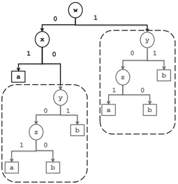
IF w= 0 AND x= 1 THEN class=a
IF y= 0 AND z = 1 THEN class=a
The three rules above cannot be represented in the form of a decision tree, as they do not have any attributes in common. Representing these rules in a decision tree would require adding unnecessary and meaningless rule terms. This is also known as the ‘replicated subtree problem’ [30, 31] illustrated in
190
Figure 2 for the two rules above.
Figure 2: An example of the replicated subtree problem for the rules: IF w = 0AND
x= 1THENclass=a,IF y= 0ANDz= 1 THENclass=a. Otherwise, class=b.
The tree structure example in Figure 2 is generated under the assumption that there exist only the four attributes (w, x, z, y); that each attribute is either associated with the value 0 or 1; and instances covered by the two rules above are classified as belonging to classa whereas the remaining rules predict class b.
This example reveals that the ‘divide-and-conquer’ rule induction ap-proach can lead to unnecessarily large and complex trees [30], whereas the Prism algorithm is able to induce modular rules such as the two rules above, that have no attribute in common. Also, the authors of [32] discuss that
200
decision tree models are less expressive, as they tend to be complex and dif-ficult to interpret by humans once the tree model grows to a certain size. Also, the authors of the well-known C4.5 decision tree induction algorithm [29] acknowledged that pruning a decision tree model does not guarantee simplicity and can still be too cumbersome to be understood by humans.
based classifiers and sometimes even outperforms decision trees (especially if the data is noisy or there are clashes in the data) [28]. Thus, Prism has been chosen as a basic rule induction strategy for Hoeffding Rules. Another
210
reason for choosing Prism is that it naturally abstains from classification, if no rule matches, whereas a decision tree based approach forces a clas-sification [9]. Abstaining may be necessary in critical applications where miss-classifications are very costly, such as in medical or financial applica-tions.
Prism follows the ‘separate-and-conquer’ approach which repeatedly ex-ecutes the following two steps: (1) induce a new rule and add it to the rule set and (2) remove all data instances covered by the new rule. The stopping criterion for executing these two steps is usually when all data instances are covered by the rule set. Hence, this approach is also often referred to as the
220
‘covering approach’. Cendrowska’s original Prism algorithm for categorical attributes implements this ‘separate-and-conquer’ approach as shown in Al-gorithm 1, where tα is a possible attribute value pair (rule term) and D is
the training data. The algorithm is executed for each classωi in turn on the
original training data D.
There have been variations of Prism, such as N-Prism which also deals with continuous attributes [28]; PrismTCS which imposes an order of the rules in the rule set [33]; PMCRI which is a scalable parallel version of PrismTCS [31] and Prism based ensemble approaches such as Random Prism [34].
230
Hoeffding Rules uses this basic Prism approach to induce rules from a recent subset of the data stream. However, different compared with Prism, Hoeffding Rules uses a more expressive representation of rule terms for con-tinuous data, which will be discussed next in Section 3.3; and also uses the Hoeffding bound to adapt the induced rule set to concept drifts in the data stream in real-time, as will be discussed in Section 3.4.
3.3. Probability Density Distribution for Expressive Continuous Rule Terms
The original Prism algorithm [12] only works on categorical attributes and produces rule terms of the form (α =ν). eRules [9] and Very Fast Deci-sion Rules (VFDR) [13] are among the few algorithms specifically developed
240
Algorithm 1:Learning classification rules from labelled data instances using Prism.
1 fori= 1→C do 2 D←Dataset;
3 whileD does not contain only instances of class ωi do 4 forall the attributes α ∈ D do
5 Calculate the conditional probability, P(ωi|tα) for all possible rule terms tα;
end
7 Select the tα with the maximum conditional probability,P(ωi|tα) as rule term;
8 D← S, create a subset S from D containing all the instances covered by tα;
end
10 The induced ruleR is a conjunction of alltα at line 7;
11 Remove all instances covered by ruleR from original Dataset;
12 repeat
13 lines 3 to 9;
untilall instances of class ωi have been removed; end
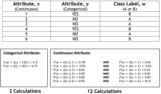
A summary of the process of how eRules and VFDR deal with continuous attributes can be described as follows:
1. For each possible value αj of a continuous attribute α, calculate the
conditional probability for a given target class for both rule terms (α < ν) and (α≥ν) or (α≤ν) and (α > ν).
2. Return the rule term, which has the overall best conditional probability for the target class.
250
It is evident that this process of dealing with continuous attributes re-quires many cut-point calculations for the conditional probabilities for each possible value αj of a continuous attribute.
Figure 3: Cut-point calculations to induce a rule term for continuous and categorical attributes.
multiplied by 2. Clearly both algorithms, eRules and VFDR, still require a lot of calculations even though the data in the example is very small. This
260
is a drawback as computationally efficient methods are needed for mining data streams. Furthermore, eRules and VFDR use a ‘separate-and-conquer’ strategy, which requires many iterations until a rule is completed.
G-eRules uses the Gaussian distribution of the attribute associated with a class label as introduced in [35], to create rule terms of the form (x < α ≤ y), and thus avoids frequent cut-point calculations. Evidence of the improvements in performance while maintaining the accuracy of the induced rules is discussed in [35]. This method is also used in the Hoeffding Rules algorithm to avoid frequent cut-point calculations. It is also more expressive than inducing rule terms from binary splits, as rule terms of the form (x < 270
α ≤y) can describe an interval of data. One would need to use two rule terms induced by binary splitting to describe the same interval of data values of a particular attribute. For each continuous attribute of the the instances, a Gaussian distribution representing all possible values of that continuous attribute for a given target class is used to generate these more expressive rule terms.
If the data instances have class labels of ω1, ω2...ωi then we can compute
the most relevant value of a continuous attribute that is the most relevant one to a particular class label based on the Gaussian distribution of the values associated with this particular class label.
280
a mean µand a varianceσ2 from all possible numeric values associated with
the class label ωi. The class conditional density probability is calculated as
in the Equation 1:
P(tα|ωi) = P(tα|µ, σ2) =
1 √
2rσ2exp(−
(tα−µ)2
2σ2 ) (1)
Hence, a heuristic based onP(ωi|tα), or equivalently log(P(ωi|tα)) is
cal-culated and used to determine the probability of a class label for a valid value of a continuous attribute as in the Equation 2:
log(P(ωi|tα)) = log(P(tα|ωi)) +log(P(ωi))−log(P(tα)) (2)
The probability between two values, Ωi, can be calculated for the range
between these two values such that if x ∈ Ωi, then x belongs to class ωi.
This method may not guarantee to capture the full details of the intricate
290
continuous attributes, but the computational and memory efficiency can be improved significantly as shown in [35] compared with binary splitting tech-nique. The efficiency as a result of using Gaussian distribution only needs to be calculated once and can be incrementally updated over time with just two variables, µ and σ2.
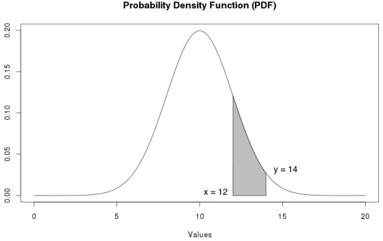
As illustrated in Figure 4, the shaded area betweenx and y should rep-resent the most common values of a continuous attribute α for class wi. A
good rule term of a continuous attribute is derived by choosing an area un-der the curve of the corresponding distribution for which the density class probability P(x < α≤y) is the greatest.
300
This technique is used to identify a possible rule term in the form of
(x < α≤ y), which is highly relevant to a range of values of the continuous
attribute αfor a target classωi from a subset of data instances. The process
can be described in the following steps:
1. Meanµand variance σ2 of each class label is calculated for each
avail-able continuous attribute.
2. Equations 1 and 2 are used to work out the class conditional density and posterior class probability for each value of a continuous attribute for a target class.
3. A value with the greatest posterior class probability is selected.
310
Figure 4: The shaded area represents a range of values of continuous attributeαfor class
ωi.
values. Choose also a greater value compared with the value selected in step 3 that also has the greatest posterior class probability among all greater values.
5. Calculate density probability with the two values in step 4 by using the corresponding Gaussian distribution calculated in step 1 for the target class.
6. Select the range of the attribute (x < α≤y) as a rule term, for which the density class probability is the maximum.
320
The normality assumption should not cause major problems if large enough sample sizes are used (>30 or 40) [36]. As stated by Altman and Bland [37], the distribution of data can be ignored if the samples consist of hundreds of observations. This is the case for data stream classifiers such as Hoeffding Rules, as they are designed for infinite data streams. Also, there are a few notable points from the central limit theorem [37, 38] regarding the normality assumption:
• If the sample data is approximately normally distributed, then the sampling distribution will also be normal distributed.
• If the sample size is large enough (> 30 or 40) then, the sampling
330
underlying distribution of the data.
From the points just mentioned above, true normality is considered to be a myth but a good estimation of normality can be confirmed by using normal plots or significance tests [37]. The main idea behind these tests is to show whether data significantly deviates from normality [36, 37, 38].
The next Section describes the adaptation of the rule induction process to data streams.
3.4. Using the Hoeffding Bound to Ensure Quality of Learnt Rules from a Data Stream
340
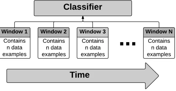
It is reasonable to assume that the recent data in a data stream is more likely to reflect the current concept more accurately compared with older data [39]. Some works [40, 41, 42, 13, 9] in data mining discuss and use a sliding windows process as illustrated in Figure 5.
Figure 5: Sliding windows process.
The fundamental idea of the sliding windows process is that a window is maintained which stores most recently seen data instances, and from which older data instances are dropped according to some set of rules. Data in-stances in a window can be used for the following three tasks [14, 43]:
1. To detect change. Using a statistical test to compare the underlying probability distribution between different sub-windows.
350
3. To rebuild or revise the learnt model after data has changed.
By using sliding windows technique, algorithms will not be affected by stale data and they can also be used as a tool to approximate the amount of memory required [1].
The proposed Hoeffding Rules algorithm usesHoeffding Inequality [16] to estimate the confidence of, whether adding a rule term to a rule, or stopping the rule’s induction process is appropriate. This makes it more likely that the rule will cover instances from the stream that match the rule’s target class. The use of Hoeffding Inequality in Hoeffding Rules was inspired by
360
[44, 45, 10]. In addition, the word ‘Hoeffding’ in our algorithm name is derived from the name of the formula called Hoeffding Inequality [16], which provides a statistical measurement in confidence of the sample mean of n
independent data instances x1, x1..., xn. If Etrue is the true mean and Eest
is the estimation of the true mean from an independent sample then the difference in probability between Etrue and Eest is bounded by Equation 3,
where R is the possible range of the difference between Etrue and Eest:
P[|Etrue−Eest|> ]<2e−2n
2/R2
(3) From the bounds of the Hoeffding Inequality, it is assumed that with the confidence of 1−δ, the estimation of the mean is within of the true mean. In other words, we have:
370
P[|Etrue−Eest|> ]< δ (4)
From Equations 3 and 4 and solving for , a bound on how close the estimated mean is to the true mean after n observations, with a confidence of at least 1−δ, is defined as follows:
=
r
R2ln(1/δ)
2n (5)
By using Hoeffding bound as an independent metric to verify the true likeness of a rule term, we say that the rules that satisfy the Hoeffding bound are likely to be as good as the rules learnt from an infinite data stream.
is calculated after the rule term with the best conditional probability for class ωi is selected. However, the rule term will be added to the current
rule unless the difference of the conditional probabilities between the selected (best) and the second best rule term is greater than . Otherwise, the rule’s
induction process is completed and the rule is added to the rule set. A new iteration for a new rule is started again with data instances covered by the previous rule removed.
IfG(tα) is the heuristic measurement that is used to test the rule termtα,
then R in Equation 5 represents the range of G(tα). G(tα) in our approach
is the conditional probability P(class=i|tα) at which a rule term tα covers
a target classωi. Hence, the probability range of a rule term R is 1. nis the
number of data instances that the rule has covered so far.
Concerning the goodness of the best rule term, let tαj be the rule term with the highest conditional probability from the current iteration, and tαj−1
390
be the rule term with the second highest conditional probability from the current iteration, then:
∆G=G(tαj)−G(tαj−1) (6)
If ∆G > , then the Hoeffding bound guarantees that with a probability
of 1−δ, the true ∆G ≥ (∆G−). If this is the case, we include the rule term into the current rule as part of Algorithm 1 at step 7 and continue to search for a new rule term if the rule still covers data instances of different classifications than the target class. Once all possible rules are induced for all class labels from the current window, then all instances covered by the rules are removed and the instances not covered are added to a temporary buffer. This buffer is then combined with the data from the next sliding window for
400
inducing new classification rules.
Essentially, we use the Hoeffding bound to determine a probability with the confidence of 1−δ that the observed conditional probability, with which the rule term covers the target class in n examples, is the same as we would observe for an infinite number of data instances.
The next section brings the previously outlined methods for rule induc-tion, dealing with continuous attributes and adaptation to concept drift to-gether.
3.5. Overall Learning Process of Hoeffding Rules
The following sections describe how we adapted and combined sliding
410
3.5.1. Inducing the Initial Classifier
The first step of Hoeffding Rules’ execution is the generation of the initial classifier, which is done in a batch mode using Prism on the firstn instances in the window. As described in Section 3.2, the Prism algorithm is able to induce expressive classification rules directly from training data by using ‘separate-and-conquer’ search strategy. The method of inducing numerical rule terms using this algorithm has been replaced with the computationally
420
more efficient way of inducing numerical rule terms, based on the Gaussian Probability Density Distributions described in Section 3.3 in this paper.
For the first window, the window size n is predefined. Subsequently the number of data instances for each window consists of unseen data instances plus the data instances not covered by the rules from the previous window. The learning process of Hoeffding Rules is described in Algorithm 2.
3.5.2. Evaluating Existing Rules and Removing Obsolete Rules
The evaluation and removal of rules is done online. Once labelled in-stances are available, then the rules of the current classifier are applied on these instances. Each rule remembers how many instances it has correctly
430
and incorrectly classified in the past. From this, the rule can update its accuracy after each classification attempt. If a rule’s classification accuracy drops below a pre-defined threshold (by default 0.8) and the rule has also taken part in a minimum number of classification attempts (by default 5), then the rule is removed. The reason for considering a minimum number of classification attempts is to avoid that the rule is removed too early.
For example, if the rule’s minimum number of classification attempts before removal is only 1, then it would be removed already if the first clas-sification attempt fails. However, with the default settings, the rule would at least ‘survive’ 5 attempts. Assuming that only the first of the 5 attempts
440
fails, then the rule would be retained, as it has an accuracy of 4÷5 = 0.8, which is the minimum classification accuracy required.
The default settings may be adjusted according to the user requirements. A lower minimum accuracy will result in the classifier adapting slower, how-ever, a high accuracy may result in rules expiring quickly, and thus more computation is required to induce new rules. Also a low number of minimum classification attempts will result in rules expiring quickly and a high number of minimum classification attempts will result in a slower adaptation. In our experiments, we have found that the default values work well in most cases. The default values have been used in all experimental results presented in
Algorithm 2: Hoeffding Rules - Inducing rules from an infinite data stream.
R← Learnt rule set;
r← A classification rule;
S← Stream of data instances;
Wunseen ← Buffer of unseen data instance;
WHB ← Buffer of data instances not covered by rules from previous
Wunseen;
n : pre-defined window size;
7 while S has more data instance do 8 i→new instance from S ; 9 if r ∈R covers ithen
10 Validate the rule r and remove if necessary; else
12 Add i toWunseen;
13
13 if Wunseen =n then
14 W0 :=Wunseen+WHB;
15 empty(Wunseen, WHB);
16 Learn rule set, R0, in batch mode as inAlgorithm 3 from
W0;
17 Add R0 toR;
18 WHB := data instances not covered by r ∈R0 in W0; end
end end
this paper.
3.5.3. Storing Data Instances that do not Satisfy the Hoeffding Bound
One of the notable features of Hoeffding Rules is the use of Hoeffding Inequality to determine the credibility of a rule term as described in Section 3.4. For an algorithm based on ‘separate-and-conquer’ strategy in batch data, a new rule term is searched and added to a current rule until the rule only covers data instances of the target class. Sliding window technique is used as described inSection 3.4to actively learn rules in real-time. The window contains the most recent training data instances, and these data instances are used to induce classification rules over time. However, Hoeffding Rules
Algorithm 3: Hoeffding Rules - Inducing rules in batch mode. 1 fori= 1→C do
2 D←input Dataset;
3 whileD contains classes other than ωi do
4 forall the α in D do
5 if α is categorical then
6 Calculate the conditional probability, P(ωi|tα) for all rule terms tα;else if α is continuous then
7 calculate mean µand varianceσ2 of continuous attributeα for class ωi;
8 foreach value αj of attributeα do
9 Calculate P(αj|ωi) based on created Gaussian distribution created in line 8;
end
11 Select αj of attribute α, which has highest value of P(αj|ωi);
12 Create tα in form of x < α≤y as bfsection 3.3;
13 Calculate P(tα|ωi), where tα is in the form ofx < α≤y;
end end
16 Calculate Hoeffding bound, =
q
R2ln(1/δ)
2∗(no. instances inD); 17 if P(tα|ωi)best−P(tα|ωi)second−best > then
18 Select tα for which P(tα|ωi) is a maximum;
else
20 Stop inducing current rule;
end
22 Create subset S of D containing all the instances covered by tα;
23 D← S;
end
25 R is a conjunction of all the rule terms built at line 17; 26 Remove all instances covered by ruleR from input Dataset;
27 repeat
28 lines 2 to 22;
untilall instances of ωi have been removed; 30 Reset input Dataset to its initial state;
end
algorithm does not always induce rules that cover only examples of the target class, because Hoeffding Rules will stop inducing further rule terms if the rule does not satisfy the Hoeffding bound metric from the current subset of data instances.
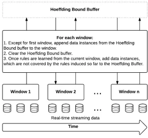
Figure 6: Combining data instances that satisfy the Hoeffding bound from the previous window with the unseen data instances from the current window.
As illustrated in Figure 6, once all possible rules are induced from the sliding window then all data instances that are not covered by the newly created rules are stored in a buffer. This buffer is combined with the next window of unseen data instances from the stream. Hence, after the first window, each sliding window is filled with unseen data instances from the window and the instances from the Hoeffding bound buffer from the previous
470
3.5.4. Addition of new Rules
The addition of new rules also takes place online. As outlined in Section 3.5.2, Hoeffding Rules applies its current rules to new data instances that are already labelled, in order to evaluate the rule set’s accuracy. However, if none of the rules applies to a labelled data instance, then this data instance is added to the window. Once the window of unseen instances reaches the defined threshold, data instances are learnt as outlined in Algorithm 2 to induce new rules, which are then added to the current classifier. Next the
480
window is reset by removing all instances from it.
This is based on the assumption that the instances in the window will primarily cover concepts that are not reflected by the current classifier. Thus, rules induced from this window will primarily reflect these missing concepts. By adding these rules to the classifier, it is expected that the classifier will adapt automatically to new emerging concepts in the data stream.
4. Experimental Evaluation and Discussion
An empirical evaluation has been conducted to evaluate Hoeffding Rules in terms of accuracy, adaptivity to concept drift and the trade off between accuracy for a white box model such as Hoeffding Rules compared with a
490
less expressive model such as Hoeffding Tree. In addition, Hoeffding Rules has also been evaluated in terms of its expressiveness compared with its more direct competitors Hoeffding Tree and VFDR. This has been accomplished empirically by measuring the number of average decision steps needed for classifying an unseen data instance, and qualitatively by examining some of the decision rules induced by Hoeffding Rules on two examples. The imple-mentation of the proposed learning system was developed in Java, using the MOA [14] environment as a test-bed. MOA stands for Massive Online Anal-ysis and is an open-source framework for data stream mining. Related to the WEKA project [46], it includes a collection of machine learning algorithms
500
4.1. Experimental Setup
Two different classifiers were used for comparing and analysing the Ho-effding Rules algorithm.
510
• VFDR(Very Fast Decision Rules) [13], is to the best of our knowledge the state-of-art in data stream rule learning.
• Hoefffding Tree[10], is state-of-art in decision tree learning from data streams.
The rationale behind this choice is twofold: (1) Hoeffding Tree has es-tablished itself for the last decade as the state-of-the-art in data stream classification, with a long history of success; and (2) both techniques use the Hoeffding bound for result approximation, which we have also adopted in
520
our technique. It is worth noting that opaque black box methods recently trialed in a data stream setting like deep learning [48] lack the expressiveness element, and thus have not been chosen for our experimental study.
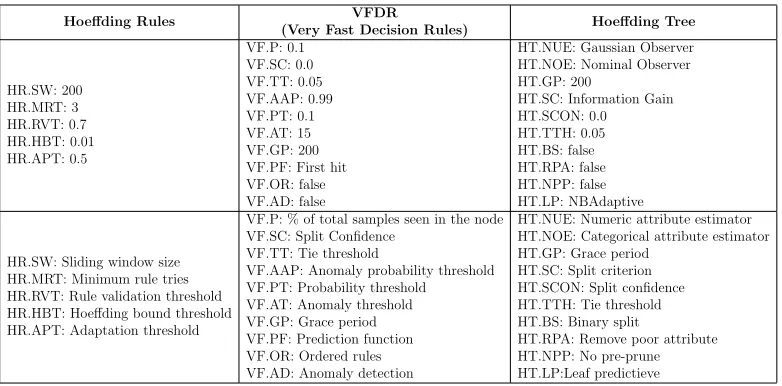
Table 1 shows the default parameters for the classifiers that were used in all of our experiments unless stated otherwise.
Table 1: Parameter settings for classifiers used in the experiments.
Hoeffding Rules VFDR
(Very Fast Decision Rules) Hoeffding Tree
HR.SW: 200 HR.MRT: 3 HR.RVT: 0.7 HR.HBT: 0.01 HR.APT: 0.5 VF.P: 0.1 VF.SC: 0.0 VF.TT: 0.05 VF.AAP: 0.99 VF.PT: 0.1 VF.AT: 15 VF.GP: 200 VF.PF: First hit VF.OR: false VF.AD: false
HT.NUE: Gaussian Observer HT.NOE: Nominal Observer HT.GP: 200
HT.SC: Information Gain HT.SCON: 0.0 HT.TTH: 0.05 HT.BS: false HT.RPA: false HT.NPP: false HT.LP: NBAdaptive
HR.SW: Sliding window size HR.MRT: Minimum rule tries HR.RVT: Rule validation threshold HR.HBT: Hoeffding bound threshold HR.APT: Adaptation threshold
VF.P: % of total samples seen in the node VF.SC: Split Confidence
VF.TT: Tie threshold
VF.AAP: Anomaly probability threshold VF.PT: Probability threshold
VF.AT: Anomaly threshold VF.GP: Grace period VF.PF: Prediction function VF.OR: Ordered rules VF.AD: Anomaly detection
HT.NUE: Numeric attribute estimator HT.NOE: Categorical attribute estimator HT.GP: Grace period
HT.SC: Split criterion HT.SCON: Split confidence HT.TTH: Tie threshold HT.BS: Binary split
4.2. Datasets
Different synthetic and real world datasets were used in our experiments. As for synthetic datasets, stream generators available in MOA were used. The real world datasets ‘Airlines’ and ‘Forest Covertype’ are known and used for batch learning, in which case all data instances from datasets are
530
read and learnt in one pass. However, we simulate these datasets into data streams by reading data instances from these dataset in ordered sequence over the time.
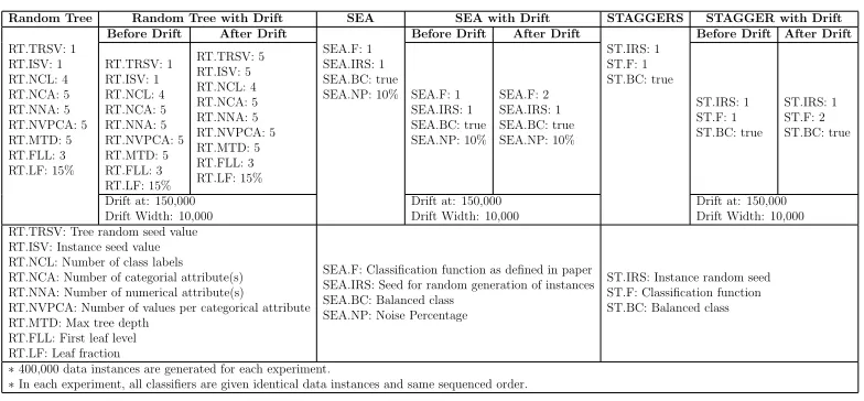
Table 2: Parameter settings for synthetic stream generators used in the experiments.
Random Tree Random Tree with Drift SEA SEA with Drift STAGGERS STAGGER with Drift
RT.TRSV: 1 RT.ISV: 1 RT.NCL: 4 RT.NCA: 5 RT.NNA: 5 RT.NVPCA: 5 RT.MTD: 5 RT.FLL: 3 RT.LF: 15%
Before Drift After Drift
SEA.F: 1 SEA.IRS: 1 SEA.BC: true SEA.NP: 10%
Before Drift After Drift
ST.IRS: 1 ST.F: 1 ST.BC: true
Before Drift After Drift
RT.TRSV: 1 RT.ISV: 1 RT.NCL: 4 RT.NCA: 5 RT.NNA: 5 RT.NVPCA: 5 RT.MTD: 5 RT.FLL: 3 RT.LF: 15% RT.TRSV: 5 RT.ISV: 5 RT.NCL: 4 RT.NCA: 5 RT.NNA: 5 RT.NVPCA: 5 RT.MTD: 5 RT.FLL: 3 RT.LF: 15% SEA.F: 1 SEA.IRS: 1 SEA.BC: true SEA.NP: 10% SEA.F: 2 SEA.IRS: 1 SEA.BC: true SEA.NP: 10% ST.IRS: 1 ST.F: 1 ST.BC: true ST.IRS: 1 ST.F: 2 ST.BC: true
Drift at: 150,000 Drift Width: 10,000
Drift at: 150,000 Drift Width: 10,000
Drift at: 150,000 Drift Width: 10,000 RT.TRSV: Tree random seed value
RT.ISV: Instance seed value RT.NCL: Number of class labels RT.NCA: Number of categorial attribute(s) RT.NNA: Number of numerical attribute(s) RT.NVPCA: Number of values per categorical attribute RT.MTD: Max tree depth
RT.FLL: First leaf level RT.LF: Leaf fraction
SEA.F: Classification function as defined in paper SEA.IRS: Seed for random generation of instances SEA.BC: Balanced class
SEA.NP: Noise Percentage
ST.IRS: Instance random seed ST.F: Classification function ST.BC: Balanced class
∗400,000 data instances are generated for each experiment.
∗In each experiment, all classifiers are given identical data instances and same sequenced order.
Each dataset used in our experiments can be summarised as follows:
• SEA artificial generator was introduced in [49] to test their stream ensemble algorithm. The dataset has two class labels and three contin-uous attributes in which one attribute is irrelevant to the class labels and underlying concept of the data stream. More information how this data stream is generated is described in [49]. [15, 13, 9] also use this
540
dataset in their empirical evaluations among other datasets.
attributes at random for splitting and assigns a random class label to each leaf. Once the tree is built, new examples are generated by as-signing uniformly distributed random values to attributes, which then determine the class label using the randomly generated tree.
550
• STAGGERwas introduced by Schlimmer and Granger [50] to test the STAGGER concept drift tracking algorithm. The STAGGER concepts are available as a data stream generator in MOA and has been used as a benchmark to test for concept drift in [50]. The dataset represents a simple block world defined by three nominal attributes size, colour and shape, each comprising 3 different values. The target concepts are:
size ≡small∧color ≡red
color ≡green∨shape≡circular
560
size ≡(medium∨large)
While performing preliminary experiments with the data stream gen-erators in MOA, it became apparent that the concepts defined did not match the ones proposed in the original paper. This was observed from the rules generated by our approach from the STAGGER data stream. Meanwhile, the ‘bug’ was reported to the MOA development team and the current, corrected implementation of the generator has been used for the experiments presented in this section. This highlights the ex-pressiveness of the rules induced by Hoeffding Rules.
570
• Forest CoverType contains the forest cover type for 30×30 meter cells obtained from US Forest Service (USFS) Region 2 Resource In-formation System (RIS) data. It contains 581,012 instances and 54 attributes, and it has been used in several papers on data stream clas-sification, i.e in [51].
• Airlines dataset was generated based on the regression dataset by Elena Ikonomovska, which consists of about 500,000 flight records. The main task of this dataset is to predict whether a given flight
580
dataset has three continuous and four categorical attributes. Elena Ikonomovska also uses this dataset in one of her studies on data streams [52]. This dataset was downloaded from the MOA website and used in our empirical experiments without any modifications.
All synthetic data stream generators are controllable by parameters and Table 2 shows the settings used for all synthetic streams in our evaluation.
4.3. Utility of Expressiveness
The empirical evaluation is focused on the cost of expressiveness when comparing the accuracy and performance between classifiers for data streams.
590
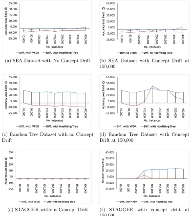
4.3.1. Accuracy Loss Band
As mentioned in [17], a learnt model from the labelled data instances may produce high predictive accuracy for unlabelled data, but the learnt model can be hard and complex to understand for human users or even domain experts. All classifiers were evaluated on the same base datasets in order to examine the trade-off between rule-based classifiers such as VFDR and Hoeffding Rules compared with tree based classifiers such as Hoeffding Tree. Concept drift was also simulated in all synthetic datasets from 150,000 data instances onwards for approximately 1,000 further instances, where both concepts were present before switching completely to the new concept. The
600
accuracy loss band ζ can be either positive or negative, where positive values indicate that Hoeffding Rules achieves a better accuracy and negative values indicate the shortfall in accuracy compared with its competitor.
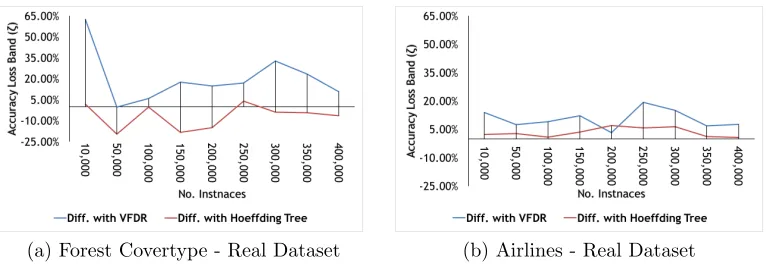
Figures 7a, 7b, 7c, 7d, 7e, 7f, 8a and 8b show that accuracy loss band ζ
of Hoeffding Rules is very competitive compared with Hoeffding Tree while clearly outperforming VFDR in most cases. The reader should note that the existing implementations of Hoeffding Tree, VFDR and synthetic data gen-erators in MOA were used, these classifiers may have been optimised to work well on these synthetic datasets. Two real datasets Airlines and CoverType are chosen and included for an unbiased evaluation. VFDR is the closest
610
(a) SEA Dataset with No Concept Drift (b) SEA Dataset with Concept Drift at 150,000
(c) Random Tree Dataset with no Concept Drift
(d) Random Tree Dataset with Concept Drift at 150,000
(e) STAGGER without Concept Drift (f) STAGGER with concept drift at 150,000
(a) Forest Covertype - Real Dataset (b) Airlines - Real Dataset
Figure 8: Difference in accuracy compared with other classifiers for real data streams.
4.3.2. Cost of Expressiveness
We also estimated the cost of expressiveness in terms of steps required for a model to predict a class label. This evaluation is focussed on the most
620
expressive rule and tree based algorithms. More decision making steps in rule and tree based algorithms implies more and potentially unnecessary and costly tests for a user to obtain a classification, which is not desirable [12, 53]. Support Vector Machines and Artificial Neural Networks based algorithms are not investigated here as they are nearly non-expressive and difficult to comprehend by human analysts. Also instance based and probabilistic mod-els are not very interesting to the human analyst in terms of expressiveness as they only indirectly explain a classification through either the enumera-tion of data instances in the case of instance based learners, or through basic probabilities in the case of probabilistic learners.
630
Classification steps for Hoeffding Rules and VFDR refer to the number of rule terms (conditions) in a rule that are needed for classifying a data in-stance. Similarly classification steps for Hoeffding Tree refer to the number of nodes that need to be visited (conditions) from the root of the tree to the leaf that provides a particular classification. As shown in Figures 9a, 9b, 9c,9d, 9e, 9f, 9g and 9h, Hoeffding Rules is more competitive in terms of number of classification steps over time compared with the Hoeffding Tree classifier. We observed in all experiments that Hoeffding Tree does not start building its tree model until several thousand data instances have been buffered to satisfy the Hoeffding Inequality. Hoeffding Tree does not limit the depth of
640
(a) SEA Dataset with No Concept Drift (b) SEA Dataset with Concept Drift at 150,000
(c) Random Tree Dataset with no Concept Drift
(d) Random Tree Dataset with Concept Drift at 150,000
(e) STAGGER No Concept Drift (f) STAGGER with concept drift at 150,000
9a, 9b, 9c,9d, 9e, 9f, 9g and 9h. In addition, we expect all three classifiers to adapt to concept drifts. The rule-based classifiers will change their rule sets, whereas Hoeffding Tree will replace obsolete subtrees with newer sub-trees. Either way, a concept drift may alter the number of steps needed to reach a classification significantly. This explains the more abrupt changes of classification steps of some algorithms for the STAGGER and Covertype data streams depicted in Figures 9f and 9h. Regarding the Covertype data
650
stream, it consists of real data and thus it is not known if there is a concept drift. However, the more abrupt changes of the number of classification steps indicates that there is a drift starting somewhere between instances 150,000 to 200,000. Thus we have used a separate concept drift detection method, a version of the Micro-Cluster based concept drift detection method presented in [54, 55], which has confirmed a drift starting at position 150,000 instances. Figures 9a, 9b, 9c,9d, 9e, 9f, 9g and 9h also compare the average number of classification steps of Hoeffding Rules with VFDR. The figures show that VFDR has a very similar average number of classification steps compared with Hoeffding Rules. For all observed cases, except for the Covertype data
660
stream, Hoeffding Rules needs an average of about 1.5 classification steps only. However, as shown in Table 3, Hoeffding Rules achieves a much higher classification accuracy than VFDR and in most cases also requires less time to learn as illustrated in Figure 11. In most cases where there is concept drift it can be seen that the number of average classification steps increases for Hoeffding Tree, whereas Hoeffding Rules’ and VFDR’s average number of classification steps stays almost constant.
The number of steps required for a classification task demonstrates the effort required to translate a classification from a tree based model into the form of an expressive ‘IF... THEN...’ rule. The current implementation of
670
Hoeffding Tree in MOA, as well as the Hoeffding Tree algorithm presented in its original paper [10], do not provide any mechanism for translating a leaf into an expressive rule. One can argue that a set of decision rules can be easily extracted from an existing tree model as Quinlan [56] has mentioned as early as in 1986. An extracted decision rule from a hierarchical model represents logic tests from a root node to a leaf. However, as Hoeffding Tree is designed to adapt to changes in data streams, this extraction process would need to repeat every time the tree expands or changes its structure. Therefore, maintaining an accurate and up-to-date rule set from a Hoeffding Tree could be a challenge and a computationally demanding task.
680
9f, we detected notable changes in the number of steps required for classi-fication using Hoeffding Tree but not for using Hoeffding Rule and VFDR. This is an expected behaviour because Hoeffding Tree may need to replace an entire subtree or in the worst case the entire tree from the root node if there is a drift in the data stream. However, rule-based classifiers such as Hoeffding Rules and VFDR do not need to replace larger numbers of rules, as rules can be examined, altered and replaced individually. Examining, re-placing and altering individual ‘rules’ (decision paths from the root node to a leaf node) is not possible in trees without also altering further ‘rules’ that
690
are connected to the rule to be changed through intermediate tree nodes. For real datasets, we do not have an absolute ground truth whether concept drifts are encoded in the data or not, but we expect to see concept drifts in real-life data streams. In particular, we saw a correlated behaviour between abstain-ing and classification steps in Figures 9h and 10 for the Covertype dataset between 150,000 and 200,000 instances. As mentioned before we have used a version of the Micro-Cluster based concept drift detection method presented in [54, 55], which confirmed a drift starting at position 150,000 instances. In this particular case Hoeffding Rules dropped slowly in the average number of steps needed for classification, and Hoeffding Tree suddenly stopped growing
700
and stalled for about 50,000 data instances before starting to grow further. Hence, we believe that Hoeffding Tree also adapted to a drift here.
4.3.3. Expressive Rules’ Ranking and Interpretation
At any given time a user can inspect the decision rules directly from the rule set produced by Hoeffding Rules and can be confident that the rules reflect the underlying pattern encoded in the data stream at any given time. For example, we extracted the top 3 rules (based on the rules’ individual classification accuracy) learnt from the two real datasets, Covertype and Airlines at 50,000 data instances:
• Covertype Dataset:
710
– IFSoil-Type40= 0ANDSoil-Type30 = 0ANDSoil-Type38 = 0THENClass= 0
– IFSoil-Type38= 1THENClass= 7
– IFSoil-Type10= 1AND0.57<Aspect<= 0.64THENClass= 6
• Airlines Dataset:
– IFAirportTo =CHAANDDayOfWeek = 3ANDAirportFrom=AT LANDAirline
– IFAirportFrom=CLT THENClass= 0
– IFAirportTo= AZOTHENClass= 1
As it can be seen, rules induced by Hoeffding Rules can be modular (independent from each other) meaning that the rules not necessarily have
720
any attributes in common, which is not possible when rules are presented in a tree structure. Rules extracted from a tree will have at least the attribute chosen to split on the root node in common, even if this attribute may not be necessary for some classification tasks. Thus a tree structure may result in potentially unnecessary and costly tests for the user. This is also known as the replicated subtree problem [30]. We refer to Section 3.2 for an explanation of the replicated subtree problem.
In addition as mentioned in Section 4.2, while performing preliminary experiments with the data stream generators in MOA, it became apparent that the concepts defined for the STAGGER generator did not match the ones
730
proposed in the original paper [50]. This further highlights the expressiveness of the rule set induced by Hoeffding Rules. This ‘bug’ was reported to the MOA development team and a corrected version of the stream generator was used for the experiments described in this paper.
4.4. Abstaining from Classification
The results presented in Section 4.3 showed the tolerance of rule-based classifiers compared with decision tree based classifiers for the utility of ex-pressiveness. Another important feature of Hoeffding Rules is the ability to abstain. In Figure 10, we observe that the abstaining rate of Hoeffding Rules decreases as Hoeffding Rules processes more instances, except for the
Ran-740
dom Tree dataset. For synthetic datasets with concept drift, we also notice that at the point of simulated concept drift (150,000), the abstaining rate spiked up but quickly recovered to adapt to the new concept. This indicates one of the major benefits of abstaining instances from classification, when Hoeffding Rules is uncertain about a classification it does not risk classifying unseen data instances. This feature is desirable or even crucial in domains and applications where miss-classification is costly or irreversible. As men-tioned before we have used a version of a Micro-Cluster based concept drift detection method presented in [54, 55], which confirmed a drift starting at position 150,000 instances.
750
Figure 10: Abstaining rates of Hoeffding Rules.
refuse a classification if the classifier is not confident to output a decisive pre-diction from its rule set. We recorded the tentative accuracy and abstaining rate for Hoeffding Rules as well as overall accuracy for Hoeffding Tree and VFDR. Tentative accuracy for Hoeffding Rules is the accuracy for instances where the classifier is confident to produce a reliable prediction. The tenta-tive accuracy was also used for estimating the utility of expressiveness shown in Section 4.3.
Table 3: Accuracy evaluation between Hoeffing Tree, VFDR and Hoeffding Rules.
Dataset
Algorithm Measure SEA Random Tree STAGGER Forest Covertype Airlines No Drift With Concept Drift No Drift With Concept Drift No Drift With Concept Drift
Hoeffding Rules
Tentative Accruacy
(%) 82.6 84.30 81.86 75.62 100 98.50 74.24 66.74 Abstaining Rate
(%) 8.07 6.43 49.51 56.02 22.27 28.52 10.04 16.47 VFDR Overall Accruacy
(%) 81.3 82.26 52.28 47.07 100 86.20 61.32 62.50 Hoeffding Tree Overall Accuracy(%) 88.08 89.23 88.98 61.08 100 99.75 82.04 66.04
We can see that Hoeffding Rules outperforms VFDR in all cases and is
760
Figure 11: Learning time Hoeffding Rules, Hoeffding Tree and VFDR.
or domain experts. Decision trees would first need to undergo a further processing step before a human user can interpret the rules. This would translate the tree into rules starting in single passes from the root node down
770
to each leaf. This may well be a too cumbersome and a too time consuming task for the decision taker.
Automating tree traversal to increase expansiveness is an additional linear process with respect to the number of tree nodes, or in its best case for balanced trees, it can be O(log(tn)) where tn is the number of nodes in the
tree [57].
4.5. Computational Efficiency
In order to examine Hoeffding Rules’ computational efficiency, we have compared Hoeffding Rules, VFDR and Hoeffding Tree on the same data streams as in Table 3. As shown in Figure 11, the execution time of Hoeffding
780
Rules outperforms that of VFDR by far and is also very close to that of Hoeffding Trees.
In summary, loosely speaking, Hoeffding Rules shows a much better per-formance in terms of utility of expressiveness compared with its direct
com-790
petitor VFDR and is also competitive compared with its less expressive com-petitor Hoeffding Tree. The same counts for the evaluation with respect to computational efficiency, Hoeffding Rules’ runtimes are much shorter com-pared with VFDR and only slightly longer comcom-pared with Hoeffding Tree.
5. Conclusions
The research presented in this paper is motivated by the fact that rule-based data stream classification models are more expressive than other mod-els, such as decision tree modmod-els, instance based models and probabilistic models. Inducing a classifier on data streams has some unique challenges compared with data mining from batch data, as the pattern encoded in the
800
stream may change over time which is known as concept drift. While most data stream mining classification techniques focus on achieving a high accu-racy and quick adaptation to concept drift, they are often rather unfriendly, cumbersome or too complex to provide trustful decisions to the users, which is undesirable in many domains such as surveillance or medical applications. This paper proposed the new Hoeffding Rules data stream classifier that focusses on producing an expressive rule set that adapts to concept drift in real-time. Compared with less expressive data stream classifiers, Hoeffd-ing Rules explains how a decision is reached. The algorithm is based on a ‘separate-and-conquer’ approach and the Hoeffding bound to adapt the rule
810
set to concept drifts in the data. Different compared with existing well es-tablished data stream classifiers, Hoeffding Rules may decide to abstain from classifying a data instance if it is uncertain about the true class label. This again is desirable in applications where a false classification label may be very costly such as in medical applications or network intrusion detection. Additionally, the abstained data instances can also be considered for active learning, which is a direction to go forward for our proposed Hoeffding Rules classifier to improve and maximise the effectiveness of the learnt model. In this way, the abstaining feature is not just reducing the miss-classification but can also potentially improve the accuracy of the overall model.
820
The evaluation measured the loss band ζ between the competitors and the speed of inducing rules on streaming data. The results show that Hoeffing Rules outperforms its direct competitor VFDR in terms of accuracy loss band and execution time. Compared with Hoeffding Tree, the proposed algorithm only showed a slight loss of accuracy and runtime. However, Hoeffding Rules produces more expressive rules compared with Hoeffding Tree and is also
830
able to abstain from classification when it is uncertain. The experimental work has shown that Hoeffding Rules provides an array of unique advantages over other stream classifiers: (1) the fastest rule-based streaming method; (2) a trusted method that effectively handles uncertainty; and (3) the most expressive stream classifier with a small ζ when compared with the closest less expressive method (Hoeffding Tree). As such and to the best of our knowledge, the reported results evidence that Hoeffding Rules is the fastest and most trustworthy stream classifier.
Acknowledgements
The findings reported in this paper are part of the ‘Fast Generalised Rule
840
Induction’ project, funded by EPSRC, Reference EP/M016870/1.
References
[1] B. Babcock, S. Babu, M. Datar, R. Motwani, J. Widom, Models and issues in data stream systems, Proceedings of the twentyfirst ACM SIG-MODSIGACTSIGART symposium on Principles of database systems PODS 02 pages (2002-19) (2002) 1. doi:10.1145/543614.543615.
[2] M. M. Gaber, A. Zaslavsky, S. Krishnaswamy, Mining data
streams: a review, SIGMOD Rec. 34 (2) (2005) 18–26.
doi:10.1145/1083784.1083789.
[3] M. M. Gaber, Advances in data stream mining, Wiley Interdisciplinary
850
Reviews: Data Mining and Knowledge Discovery 2 (1) (2012) 79–85. doi:10.1002/widm.52.
[5] H. Kargupta, B.-h. Park, S. Pittie, L. Liu, D. Kushraj, K. Sarkar, Mo-biMine: Monitoring the stock market from a PDA, ACM SIGKDD Ex-plorations Newsletter 3 (2) (2002) 37–46.
[6] H. Kargupta, R. Bhargava, K. Liu, M. Powers, P. Blair, S. Bushra, J. Dull, K. Sarkar, M. Klein, M. Vasa, D. Handy, VEDAS: A Mobile and Distributed Data Stream Mining System for Real-Time Vehicle
Moni-860
toring, in: International SIAM Data Mining Conference, Vol. 23, 2004, pp. 300–312.
[7] P. Kadlec, B. Gabrys, S. Strandt, Data-driven Soft Sensors in the process industry, Computers and Chemical Engineering 33 (4) (2009) 795–814. doi:10.1016/j.compchemeng.2008.12.012.
[8] M. Adedoyin-Olowe, M. M. Gaber, F. Stahl, TRCM: A Methodol-ogy for Temporal Analysis of Evolving Concepts in Twitter, in: Ar-tificial Intelligence and Soft Computing, no. 7895, 2013, pp. 135–145. doi:10.1007/978-3-642-38610-7 13.
[9] F. Stahl, M. M. Gaber, M. M. Salvador, eRules: A modular adaptive
870
classification rule learning algorithm for data streams, Res. and Dev. in Intelligent Syst. XXIX: Incorporating Applications and Innovations in Intel. Sys. XX - AI 2012, 32nd SGAI Int. Conf. on Innovative Techniques and Applications of Artificial Intel. (2012) 65–78doi:10.1007/978-1-4471-4739-8-5.
[10] P. Domingos, G. Hulten, Mining high-speed data streams, Pro-ceedings of the sixth ACM SIGKDD international conference on Knowledge discovery and data mining - KDD ’00 (2000) 71– 80doi:10.1145/347090.347107.
[11] H. Yang, S. Fong, Moderated VFDT in stream mining using adaptive tie
880
threshold and incremental pruning, in: Data Warehousing and Knowl-edge Discovery, Springer, 2011, pp. 471–483.
[12] J. Cendrowska, PRISM: An algorithm for inducing modular rules (1987). doi:10.1016/S0020-7373(87)80003-2.
[14] A. Bifet, G. Holmes, B. Pfahringer, P. Kranen, H. Kremer, T. Jansen, T. Seidl, MOA: Massive Online Analysis, a framework for stream clas-sification and clustering.
890
[15] A. Bifet, G. Holmes, B. Pfahringer, R. Kirkby, R. Gavald`a, New en-semble methods for evolving data streams, Proceedings of the 15th ACM SIGKDD international conference on Knowledge discovery and data mining - KDD ’09 (2009) 139doi:10.1145/1557019.1557041.
[16] W. Hoeffding, Probability inequalities for sums of bounded random vari-ables, Journal of the American Statistical Association 58 (301) (1963) 13–30. arXiv:0603030, doi:10.1080/01621459.1963.10500830.
[17] I. Zliobaite, A. Bifet, M. Gaber, B. Gabrys, Next challenges for adap-tive learning systems, SIGKDD Explorations 14 (1) (2012) 48–55. doi:10.1145/2408736.2408746.
900
[18] M. T. Ribeiro, S. Singh, C. Guestrin, Why should i trust you?: Explain-ing the predictions of any classifier, in: ProceedExplain-ings of the 22nd ACM SIGKDD International Conference on Knowledge Discovery and Data Mining, ACM, 2016, pp. 1135–1144.
[19] A. Nguyen, J. Yosinski, J. Clune, Deep neural networks are easily fooled: High confidence predictions for unrecognizable images, in: Proceedings of the IEEE Conference on Computer Vision and Pattern Recognition, 2015, pp. 427–436.
[20] G. Hulten, P. Domingos, VFML–a toolkit for mining high-speed time-changing data streams, Software toolkit (2003) 51.
910
[21] G. Widmer, M. Kubat, Learning in the presence of concept drift and hidden contexts, Machine Learning 23 (1) (1996) 69–101. doi:10.1007/BF00116900.
[22] M. a. Maloof, R. S. Michalski, Incremental learning with partial instance memory, Artificial Intelligence 154 (1-2) (2004) 95–126. doi:10.1016/j.artint.2003.04.001.
[24] P. Kosina, J. Gama, Very fast decision rules for classification in data streams, Data Mining and Knowledge Discovery 29 (1) (2015) 168–202.
920
[25] M. Deckert, Incremental rule-based learners for handling concept drift: an overview, Foundations of Computing and Decision Sciences 38 (1) (2013) 35–65.
[26] W. W. Cohen, Fast effective rule induction, Proceedings of the Twelfth International Conference on Machine Learning (1995) 115– 123doi:10.1.1.50.8204.
[27] J. R. Quinlan, Improved use of continuous attributes in C4.5, Jour-nal of Artificial Intelligence Research 4 (1996) 77–90. arXiv:9603103, doi:10.1613/jair.279.
[28] M. Bramer, Automatic Induction of Classification Rules from Examples
930
Using N-Prism, in: Research and Development in Intelligent Systems XVI, Springer London, 2000, pp. 99–121.
[29] J. R. Quinlan, C4.5: Programs for Machine Learning, Vol. 1, 1993. doi:10.1016/S0019-9958(62)90649-6.
[30] I. H. Witten, E. Frank, Data Mining: Practical machine learning tools and techniques, 2005.
[31] F. Stahl, M. Bramer, Computationally efficient induction of classifi-cation rules with the PMCRI and J-PMCRI frameworks, Knowledge-Based Systems 35 (2012) 49–63. doi:10.1016/j.knosys.2012.04.014. [32] J. F¨urnkranz, D. Gamberger, N. Lavraˇc, Foundations of rule learning,
940
no. 2003, 2012. doi:10.1007/978-3-540-75197-7.
[33] M. Bramer, An information-theoretic approach to the pre-pruning of classification rules, in: Intelligent information processing, Springer, 2002, pp. 201–212.
[35] T. Le, F. Stahl, J. B. Gomes, M. M. Gaber, G. Di Fatta, Computation-ally Efficient Rule-Based Classification for Continuous Streaming Data, in: Research and Development in Intelligent Systems XXIV, 2008, p.
950
2014. doi:10.1007/978-1-84800-094-0.
[36] J. Pallant, SPSS Survival Manual: A step by step guide to data analysis using SPSS, Vol. 3rd, 2010.
[37] D. G. Altman, J. M. Bland, Statistics notes: the normal distribution., BMJ (Clinical research ed.) 310 (1995) 298. doi:10.1136/bmj.310.6975.298.
[38] A. C. Elliott, W. A. Woodward, Statistical Analysis Quick Reference Guidebook: With SPSS Example (2007). doi:10.4135/9781412985949. [39] W. N. Street, Y. Kim, A streaming ensemble algorithm (SEA) for
large-scale classification, Proceedings of the seventh ACM SIGKDD
interna-960
tional conference on Knowledge discovery and data mining - KDD ’01 4 (2001) 377–382. doi:10.1145/502512.502568.
[40] L. Q. L. Qiao, D. Agrawal, A. E. Abbadi, Supporting slid-ing window queries for continuous data streams, 15th Interna-tional Conference on Scientific and Statistical Database Management, 2003.doi:10.1109/SSDM.2003.1214970.
[41] W.-p. Chen, S. Member, Dynamic Clustering for Acoustic Target Track-ing in Wireless Sensor Networks, IEEE Transaction On Mobile Comput-ing 3 (2004) 258–271. doi:10.1109/TMC.2004.22.
[42] M. Ali, M. Mokbel, W. Aref, I. Kamel, Detection and tracking of discrete
970
phenomena in sensor-network databases, in: Proceedings of the 17th In-ternational Conference on Scientific and Statistical Database Manage-ment (SSDBM), 2005, pp. 163–172.
[45] O. Maron, A. Moore, Hoeffding Races: Accelerating Model Selection Search for Classification and Function Approximation, Advances in Neu-ral Information Processing Systems (1993) 59–66.
980
[46] M. Hall, E. Frank, G. Holmes, B. Pfahringer, P. Reutemann, I. H. Wit-ten, The WEKA data mining software: an update, ACM SIGKDD ex-plorations newsletter 11 (1) (2009) 10–18.
[47] J. Gama, R. Sebasti˜ao, P. P. Rodrigues, On evaluating stream learning algorithms, Machine Learning 90 (3) (2013) 317–346. doi:10.1007/s10994-012-5320-9.
[48] J. Read, F. Perez-Cruz, A. Bifet, Deep learning in partially-labeled data streams, in: Proceedings of the 30th Annual ACM Symposium on Ap-plied Computing, ACM, 2015, pp. 954–959.
[49] W. N. Street, Y. Kim, A streaming ensemble algorithm (SEA) for
large-990
scale classification, in: Proceedings of the seventh ACM SIGKDD in-ternational conference on Knowledge discovery and data mining, ACM, 2001, pp. 377–382.
[50] J. C. Schlimmer, R. H. Granger, Beyond Incremental Processing: Track-ing Concept Drift, in: AAAI, 1986, pp. 502–507.
[51] H. Abdulsalam, D. B. Skillicorn, P. Martin, Streaming Ran-dom Forests, in: Proceedings of the International Database Engi-neering and Applications Symposium, IDEAS, 2007, pp. 225–232. doi:10.1109/IDEAS.2007.4318108.
[52] E. Ikonomovska, J. Gama, S. Dˇzeroski, Learning model trees from
evolv-1000
ing data streams, Data Mining and Knowledge Discovery 23 (2010) 128– 168. doi:10.1007/s10618-010-0201-y.
[53] M. Bramer, Principles of data mining, Springer, 2016.
[54] M. Hammoodi, F. Stahl, M. Tennant, Towards online concept drift de-tection with feature selection for data stream classification, in: 22nd European Conference on Artificial Intelligence, 2016, pp. 1549–1550.