Type of the Paper (Article)
1
Estimates of the leaf area index using unmanned
2
aerial vehicle images of an urban mangrove in the
3
Vitória Bay, Brazil
4
Elizabeth Dell’Orto e Silva
1*,
Alexandre Candido
Xavier
2,
Angélica Nogueira de
5
Souza Tedesco
3,
Aurélio Azevedo Barreto Neto
3,
Luiz Eduardo Martins de Lima³
,
6
José Eduardo Macedo
Pezzopane
2, and
Mônica Maria Pereira Tognella
1.
7
1Postgraduate Program in Oceanography, Federal University of Espírito Santo, Espírito Santo, Brazil;
8
lisadellorto@gmail.com; monica.tognella@gmail.com
9
2Department of Forestry and Wood Sciences, Federal University of Espírito Santo, Espírito Santo, Brazil;
10
alexandre.candido.xavier.ufes@gmail.com; pezzopane2007@yahoo.com.br
11
3Federal Institute of Espírito Santo, Espírito Santo, Brazil; aurelio@ifes.edu.br; angelica.nst@gmail.com;
12
luisedu@ifes.edu.br
13
14
* Correspondence: lisadellorto@gmail.com; Tel.: +55-27-9922-60495
15
16
Abstract: The urban mangrove of the Vitória Bay, Espírito Santo, Southern Brazil suffers from
17
anthropogenic impacts, which interfere in the foliar spectral response of its species. Identifying the
18
spectral behavior of these species and creating regression models to indirectly obtain structure data
19
like the Leaf Area Index (LAI) are powerful environmental monitoring tools. In this study, LAI was
20
obtained in 32 plots distributed in four stations. In situ LAI regression analysis with the SAVI
21
resulted in significant positive relationships (r² = 0.58). Forest variability regarding the degree of
22
maturity and structural heterogeneity and LAI influenced the adjustment of vegetation indices
23
(VIs). The highest regression values were obtained for the homogeneous field data, represented by
24
R. mangle plots, which also had higher LAI values. The same field data were correlated with SAVI
25
of a RapidEye image for comparison purposes. The results showed that, images obtained by a UAV
26
have higher spatial resolution than the Rapideye image, and therefore had a greater influence of the
27
background. Another point is that the statistical analysis of the field data with the IVs obtained
28
from the RapidEye image did not present high regression coefficient (r² = 0.7), suggesting that the
29
use of VIs applied to the study of urban mangroves needs to be better evaluated, observing the
30
factors that influence the leaf spectral response.
31
32
Keywords: UAV images; mangrove; vegetation indices; Leaf Area Index (LAI)
33
34
35
36
1. Introduction
37
The Leaf Area Index (LAI) is defined as the total leaf area projected per area unit of land (m2/m2)
38
[1]. This index allows calculations based on plant biomass and characterization of the canopy
39
architecture, two structural parameters that provide information on the vigor of the vegetation
40
cover. These estimates enable evaluating the physiognomic and physiological conditions of the
41
canopies, as well as quantitative and qualitative analyses of energy and matter flows [2].
42
Remote sensing studies using orbital sensors established relationships between vegetation
43
indices (VIs) and LAI [3–5], as well as other biophysical information like biomass, canopy density
44
[6–8], and species distribution [9,10].
45
LAI estimates using remote sensing techniques are affected by the soil type and shade, which
46
may distort the results, usually resulting in decreased reflected radiance [11]. Besides, factors that
47
can affect the spectral behavior of a vegetation canopy include the type of vegetation cover;
48
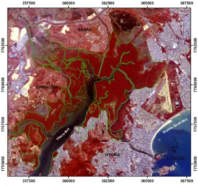
orientation and spacing of trees; canopy morphology; internal structure of canopy elements; tree
49
crown diameter; tree height; water content of plant and soil; plant health conditions; zenith and
50
azimuth solar angles; latitude; and resolution of the equipment used [12].
51
The Soil-Adjusted Vegetation Index (SAVI) seeks to mitigate the effects of soil background. It
52
was proposed based on studies carried out under different conditions of soil and vegetation cover
53
(Huete 1988), as:
54
55
𝑆𝐴𝑉𝐼 =(( )( )),
56
57
where ρIV and ρV are the reflectances of bands 4 and 3 of the Landsat 5 satellite, and L can vary from
58
0.1 to 0.5 according to characteristics of the analyzed canopy.
59
SAVI is based on the principle that the vegetation curve tends to approach the soil curve for low
60
vegetation densities but varies the spectral responses in medium vegetation densities until there is
61
almost no soil influence on high vegetation densities [13]. The SAVI equation is similar to that of the
62
Normalized Difference Vegetation Index (NDVI) [14] plus a constant, L, which varies from 0 to 1
63
according to the degree of greater or lesser soil coverage, respectively. Likewise, there are three other
64
modifications of the SAVI, the Transformed SAVI (TSAVI) [15,16], Modified SAVI (MSAVI) [17], and
65
Optimized SAVI (OSAVI) [18].
66
Zhang et al. [19] discussed that, with the advent of hyperspectral sensors, other spectral indices
67
had been developed. These include the Pigment Simple Ratio (PSR), which analyzes photosynthetic
68
pigments and the Structure Insensitive Pigment Index (SIPI), which examines the structure and
69
water content.
70
Working with VIs also requires radiometric calibration. Calibration is the process of
71
transforming the digital number (DN) of each image pixel into values of physical parameters like
72
radiance or reflectance [20].
73
The reflectance of a target can be described as a function of the wavelength and the directions of
74
irradiation and observation, thus named Bidirectional Reflectance Distribution Function (BRDF)
75
[21]. The BRDF correction process takes into account the changes of the energy recorded in the
76
images caused by differences in geometry and instantaneous image acquisition, the anisotropy of
77
the targets, information on solar and sensor angles, and shared points in images [22].
78
In the radiometric calibration of aerial photographs obtained with unmanned aerial vehicles
79
(UAVs), the process is carried out for each photo, and not for the whole scene as for the orbital
80
images. Variations in the Global Navigation Satellite System (GNSS) and UAV inertial systems can
81
produce variations of the zenith angle (θv). According to [23], it is impossible to conduct directional
82
measurements of canopies in the laboratory, and it is complicated to implement directional
83
reflectance measurements in the open air. However, digital aerial photos, when taken with high
84
frontal and lateral overlap, provide a convenient tool for analyzing the effects of directional
85
reflectance.
86
Several authors have found positive correlations between LAI estimates collected in the field
87
and VIs (e.g., NDVI) derived from satellite images [3,24], suggesting that highly accurate LAI
88
thematic maps can be repeatedly derived from these sensors in considerable areas without the need
89
for a high number of ground measurements. Most studies have been conducted in well-developed
90
mangrove forests and, consequently, the robustness of such relationships in less ideal conditions,
91
i.e., in plots of urban mangroves, also needs to be studied [25].
92
Therefore, this study aimed to test the feasibility of using a UAV to extract information from the
93
Correlation analysis was performed between the data collected in situ (LAI, diameter at breast height
95
(DBH), tree height, and density of individuals) and VIs (NDVI, SAVI) from images taken by a UAV.
96
VIs were also calculated using a Rapideye satellite image, and the correlation analysis was performed
97
with the same field data to compare the results.
98
The results showed that, even for the satellite images, the correlation analysis did not have a
99
high coefficient of determination (r2), suggesting that forest variability regarding the degree of
100
maturity and structural heterogeneity and LAI influenced VIs adjustment. The highest regression
101
values were obtained for the SAVI image with the most homogeneous field data, represented by R.
102
mangle plots, which also had higher LAI values.
103
2. Materials and Methods
104
Four study areas were defined in the mangrove of the Vitória Bay, which extends through the
105
municipalities of Vila Velha, Cariacica, Serra, and Vitória. The delimited areas are located in the
106
municipality of Cariacica, with ~ 15 ha each (Figure 1). For each study area, there were eight field
107
plots, totaling 32. The criteria for choosing these areas considered the localization of the Vitória
108
airport and suitable places for takeoff and landing of the UAV.
109
110
111
112
Figure 1. Location of the mangrove of the Vitória Bay, Espírito Santo State, Southeastern Brazil, and
113
the four study areas.
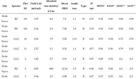
114
115
The UAV used was an X700 hexacopter measuring 1.05 m x 0.72 m and weighing 3 kg without
116
battery and gimbal. The battery (LIPO 5200mah to 6000mah 4S Tattu) allows autonomy of 13' of
117
flight. The UAV was equipped with a Tetracam ADC Snap multispectral camera (Tetracam, Inc.,
118
Gainesville, USA) weighing 90 g. This camera has three channels with a Charge Coupled Device
119
(CCD) resolution of 1,280 x 1,024 pixels, 10-bit radiometric resolution, 5-micron pixel size, and 8.43
120
mm focal length. The aperture was set at f/3.2, with 110% exposure time and y~ 2'' capture time.
121
Tetracam ADC Snap is a non-metric, small format camera with green, red, and near-infrared (520
122
nm – 920 nm).
123
LAI was obtained using the LAI 2000 Plant Canopy Analyzer (LI-COR, Inc., Lincoln, USA). LAI
124
measurements per plot. Measurements were performed in zigzags takes along the transverse line of
126
the plots. Subsequently, mean measurements for each plot were calculated. Structural data of the
127
forest were collected from June 2016 to July 2016 for each of the study areas. Tree height was
128
obtained using a Vertex Laser apparatus (Haglöf, Inc., Madison, USA), and the diameter with a
129
calibrated Forestry Suppliers Metric Fabric diameter tape, model 283D/10M (Forestry Suppliers, Inc.,
130
Jackson, USA), thus producing direct readings instead of circumference data. Each study area
131
included eight plots of 10 m x 10 m, totaling 32 plots, which were used to evaluate the different
132
structures representing the forest canopy. The methodology used to obtain and analyze structural
133
data was described by Schaeffer-Novelli and Cintron [26]. The coordinates of the plot vertices were
134
measured with a GNSS Trimble® R4 (Trimble Inc., California, USA) to prepare a georeferenced
135
shapefile in a Geographic Information System.
136
Shorter and individual flights over each area were planned, considering the autonomy time of
137
the equipment flight and the distribution of study areas. The flight plan was prepared using the free
138
software Mission Planner v 1.3.41 [27]. The flights were executed in October 2016. Geometric
139
rectification was performed with a block adjustment using information on exterior orientation
140
collected during flight with a Global Positioning and Inertial Navigation System (GPS/INS)
141
instrumentation and GPS measurements with ground control points (GCPs). GCPs were measured
142
using a pair of Trimble brand RTK4 GNSS signal receivers, configured with 15° elevation mask and
143
1'' recording rate. The screening method used was the rapid static, with an occupation time of y~ 5'.
144
The base receiver received real-time corrections from the coordinates database of the Brazilian
145
Institute of Geography and Statistics ("Instituto Brasileiro de Geografia e Estatística"- [28]) through
146
telephone signal. The data were processed in Datum SIRGAS 2000 using the UTM projection system,
147
zone 24, -39º central meridian. Data were downloaded to the Trimble Business Center software [29]
148
and exported to a Microsoft Excel© spreadsheet. The ellipsoidal height was transformed to
149
orthometric altitudes by calculating the geoid undulation in the free software Mapgeo 2015 v 1.0
150
[28].
151
Orthomosaic maps were generated for each band separately in the Agisoft Photoscan
152
Professional v 1.2.4 [30]. This software performs internal orientation, automated correspondence
153
between all overlapping images, and simultaneous bundle block adjustment; besides, it produces
154
Digital Surface Models (DSM), Digital Terrain Models (DTM), and orthomosaics. User interventions
155
are necessary to define some parameters such as the correspondence processing method, density of
156
DTM points, and the size of the smallest element in the terrain [30].
157
The radiometric calibration process was based on converting the DN of the images into a
158
reflectance factor. The spectral characterization of the calibration target (reference surface) was
159
obtained using a FieldSpec Pro model spectroradiometer (Analytical Spectral Devices, Inc.,
160
Longmont, USA). This is a portable instrument that can capture spectral data from 350 nm to 2500
161
nm with a spectral resolution of 1 nm.
162
An E.V.A. (ethyl vinyl acetate) plate was used as the absolute reference standard because this
163
material shows uniform reflectance to the wavelengths of the used sensors, highly similar to the
164
spectral behavior of a Spectralon plate. During data acquisition, the pistol of the spectroradiometer
165
formed an orthogonal incidence angle with the E.V.A. plate. Three spectral measurements were
166
taken, one at the beginning, one during, and one at the end of the flight.
167
The reflectance of the reference plate was calculated by weighting the spectral response of the
168
mean radiometric measurements on the plate to the narrow bands 560 nm (B1), 660 nm (B2), and 830
169
nm (B3), with a Full-Width at Half Maximum (FWHM) of 10 nm. The spectral sensitivity function of
170
the sensor, known as Spectral Response Function (SRF), can be simulated in the form of a Gaussian
171
function, corresponding to the maximum efficiency of the sensor in a given band. SRF can be
172
calculated using the spectral response of the target [31].
173
The DN conversion of each component, B1, B2, and B3, into the reflectance factor, was
174
performed separately using Matlab v. R2015b [32] image processing environment based on the
175
equation suggested by Miura and Huete [33], as follows:
176
𝑅 = ( ɵ)( )∗ 𝑅𝑟,
178
179
where DNt is the DN of the image reference plate; DNr is the DN of the image where the reference
180
plate is located, and Rr is the reflectance factor of the reference plate measured with the
181
spectroradiometer during flight.
182
The RapidEye Analytic Orthoimage is a multispectral, orthorectified image provided by Planet©
183
[34]. The image was acquired on October 8, 2016, at 13:23 h (UTC) at nadir. The radiometric
184
calibration process was performed in ENVI v 5.1 using the Fast Line-of-sightAtmospheric Analysis of
185
Hypercubes (FLAASH algorithm) [35]. All bands were transformed from DN to radiance
186
measurements at the top of the atmosphere, and later to reflectance values. This conversion is only
187
possible for scenes with metadata files (MTL), allowing the process of the following equation [35]:
188
189
𝐿𝜆=𝐺ai𝑛∗𝑝𝑖𝑥𝑒𝑙𝐷𝑁 +𝑜𝑓𝑓𝑠𝑒t.
190
191
The raster calculator available at ArcGIS Desktop v 10.1 [36] was used to perform arithmetic
192
operations between the spectral bands and to generate the NDVI and SAVI spectral indices of both
193
the UAV and Rapideye images. Then, in this same software, shapefiles of the plot polygons (10 m x 10
194
m) were created from coordinate points measured in the field with a Trimble RTK4 GPS. The images
195
of the spectral indices were cut using the shapefiles, and the mean values of these indices were
196
determined for each plot.
197
The relationships between the dependent variables LAI, tree height, density of individuals, and
198
DBH obtained in situ and the independent variables NDVI and SAVI calculated based on the images
199
were tested, one by one. The regression analysis required success in both the F-test and the T-test to
200
determine the regression modeling result. The modeling method of simple linear regression was
201
used in the regression analysis. The accuracy value of the regression model was obtained by
202
calculating the standard errors of the estimated value. This error can be converted to minimum and
203
maximum precisions with 95% confidence level. The maximum precision value was used to
204
compare the precision of each model.
205
206
3. Results
207
NDVI and SAVI maps were elaborated for four sites in the mangrove. In each site, eight plots
208
were established in the field, totaling 32 plots. In the processing of aerial photos obtained by UAV,
209
there were some problems, and five plots did not have the aerial overlay. In the NDVI map, the
210
mangrove clearings showed high index values due to the wet soil and organic matter content. In the
211
SAVI map, the 0.5 adjustment factor was used, and a better result was obtained when compared to
212
the NDVI map. It was possible to separate the clearings from the canopy, and the index values for L.
213
racemosa were lower than for R. mangle, allowing species discrimination and identification of the
214
succession pattern (Figure 2).
215
217
Figure 2. NDVI and SAVI images of the four study areas from the urban mangrove of the
218
Vitória Bay, Espírito Santo State, Southeastern Brazil: (a) Santa Maria; (b) Areia Branca; (c) Porto
219
Santana; and (d) Porto Novo.
220
221
The structural data collected in the field and the spectral indices obtained from the orthomosaic
222
and Rapideye images are in Table 1. The plot structure data were converted into estimates of basal
223
area dominance per plot (Figure 3), i.e., the soil area occupied by individual biomass. Rhizophora
224
mangle was dominant in most of the plots, particularly in Santa Maria; on the other hand, L. racemosa
225
was dominant only in eight plots.
226
227
228
Table 1. Structure and spectral data of the study stations in the urban mangrove of the Vitória
229
Bay, Espírito Santo State, Southeastern Brazil. RZ, Rhizophora mangle; LAG, Laguncularia racemosa;
230
LAI, Leaf Area Index; DBH, Diameter at Breast Height; Fr, Fringe mangrove; B, Basin mangrove; H,
231
height.
232
233
Site Species Plot ID
Field LAI
(m2/m2)
Absolute
tree density/
0.1 ha
Mean
DBH
trunk/
tree
Type H (m)
NDVI* SAVI* NDVI** SAVI**
Porto
Novo
RZ 101 1.97 4.6 7.8 1.1 Fr 4.57 0.54 0.45 0.84 0.49
Porto
Novo
RZ 102 2.24 2.4 7.48 1.0 Fr 5.19 0.54 0.43 0.82 0.46
Porto
Novo LAG 10 2.06 7.9 5.02 1.15 B 6.21 0.55 0.34 0.73 0.35
Porto
Novo LAG 11 2.27 5.1 9.32 1.1 B 10.7 0.56 0.36 0.79 0.41
Porto
Novo LAG 2 1.82 5.7 5.91 1.2 B 5.07 0.49 0.34 0.6 0.3
Porto
Novo RZ 3 0.85 800 12.24 1.5 B 6.98 0.42 0.28 0.6 0.3
Santana
Porto
Santana
RZ 4 1.68 1.2 15.7 1.0 B 13.47 0.59 0.38 0.82 0.45
Porto
Santana
LAG 5 1.48 5.4 8.21 1.0 B 13.08 0.63 0.33 0.76 0.34
Porto
Santana RZ 7 2.22 2.4 8.33 1.1 B 15.13 0.59 0.41 0.87 0.5
Porto
Santana RZ 100 1.82 7.3 5.96 1.0 Fr 4.4 0.59 0.40 0.82 0.49
Porto
Santana RZ 2 1.49 2.6 12.42 1.0 B 8.16 0.61 0.36 0.79 0.44
Porto
Santana RZ 3 2.61 900 22.66 2 Fr 18.6 0.59 0.42 0.84 0.53
Porto
Santana RZ 4 3.93 9.8 3.88 1 B 5.41 0.64 0.40 0.84 0.47
Areia
Branca LAG 1 1.57 6.1 10.19 1.3 Fr 9.73 0.66 0.32 0.77 0.37
Areia
Branca
RZ 6 2.36 2.2 12.28 2.7 B 10.55 0.60 0.36 0.87 0.47
Areia
Branca RZ 5 2.88 3 7.68 1.1 Fr 4.95 0.62 0.41 0.88 0.49
Areia
Branca
RZ 7 2.26 1.1 17.42 1.3 Fr 12.1 0.57 0.43 0.84 0.50
Areia
Branca
RZ 9 1.92 1.3 9.51 1.3 Fr 8.5 0.62 0.33 0.85 0.46
Areia
Branca LAG 11 2.12 6.5 5.43 1.3 B 5.22 0.63 0.28 0.72 0.31
Areia
Branca LAG 1000 1.65 7.2 5.26 1.5 B 4.07 0.56 0.28 0.61 0.25
Areia
Branca RZ 20 2.77 1.5 13.29 1.3 Fr 13.13 0.57 0.40 0.85 0.49
Santa
Maria RZ 2 2.39 2.2 9.69 1.3 Fr 6 0.63 0.37 0.85 0.48
Santa
Maria
RZ 3 3.03 3.2 11.28 1.2 B 6.56 0.56 0.45 0.86 0.47
Santa
Maria
RZ 30 2.33 1 15.15 1.3 Fr 9.92 0.59 0.45 0.85 0.51
Santa
Maria
RZ 31 2.42 1.8 15.6 2.2 B 10.98 0.61 0.41 0.87 0.50
Santa
Maria RZ 20 2.03 1.8 12.31 1.4 B 11.68 0.61 0.33 0.84 0.45
* VANT;**RapidEye
Forest density was negatively correlated with mean DBH (r=-0.78; p <0.05; Spearman's test).
237
These results are in line with the assumption that the density is reduced in more mature forests
238
when the mean DBH value becomes higher [26]. Few trees of larger diameters characterize these
239
forests.
240
241
242
243
244
Figure 3. The dominance of individuals of Avicennia schaueriana (Av), Laguncularia racemosa
245
(Lg), and Rhizophora mangle (Rh) in the four study areas from the urban mangrove of the Vitória Bay,
246
Espírito Santo State, Southeastern Brazil.
247
248
249
Figure 4 shows a chart of the height and mean diameter of the plots measured in the field for
250
each study area. It is possible to observe the structural variability between them. Concerning the
251
LAI, the mean value was 2.08 for the plots analyzed, 2.25 for R. mangle, and 1.74 for L. racemosa. It is
252
worth mentioning that, although the measurements were carried out in October, a typical rainy
253
month in Southeastern Brazil, October 2016 was an atypical month with precipitation values of 125
254
mm and evapotranspiration of 17 mm [37].
255
258
Figure 4. Mean values of tree height (m) and mean diameter (cm) for each plot in the study
259
areas in the urban mangrove of the Vitória Bay, Espírito Santo State, Southeastern Brazil.
260
261
262
Correlation analysis led to the identification of LAI as the only dependent variable that was a
263
candidate for regression since the others (tree height, density of individuals, and DBH) were not
264
significantly correlated with the independent variables NDVI and SAVI. The highest value was
265
obtained for the regression of the variable LAI x SAVI (r2 = 43%) with a significant coefficient since
266
when analyzing the statistical significance of the Student's t-test, the null hypothesis of
267
non-significance was rejected (p-value <0.05).
268
Table 2 shows that the regression analysis of the in situ LAI variable with NDVI and SAVI
269
resulted in significant positive relationships, with SAVI presenting the best result. When analyzing
270
only the plots 100% dominated by R. mangle or L. racemosa, the r2 of LAI x SAVI increased to 0.53. In
271
the analysis of the data using only the R. mangle plots, the r2 values were 0.58 for SAVI.
272
273
274
Table 2. The coefficient of determination (r²) of the regression of the leaf area index (LAI)
275
dependent variable and the independent variables NDVI and SAVI, using Unmanned Aerial Vehicle
276
(UAV) and Rapideye images.
277
278
Dependent
variable Statistics
Independent variables Species dominance
in plots Images
NDVI (r²) SAVI (r²)
LAI r² 0.23 0.43 > 90% (L. racemosa
and R. mangle)
UAV
p-value (α) 0.01 0.00
LAI r² 0.07 0.53 100% (L. racemosa
and R. mangle)
p-value (α) 0.22 0.00
LAI r² 0.36 0.58 only R. mangle
p-value (α) 0.06 0.01
r² 0.7 0.7
only R. mangle Rapideye
LAI p-value (α) 0.002 0.003
Figure 5 shows the reflectance image (RapidEye) with RGB 532 composition. Bands 5 (NIR) and
281
3 (RED) were used to elaborate NDVI and SAVI maps.
282
283
284
Figure 5. Reflectance image (RapidEye) with RGB 532 composition.
285
286
287
Figure 6 shows the difference between the two sensors regarding spatial resolution. The
288
Tetracam ADC Snap sensor has the pixel size of 5 mm, whereas the RapidEye sensor has the pixel size
289
of 5 m. There are also differences in spectral resolution. The Tetracam ADC Snap camera sensor
290
displays the RED and NIR bands centered at 660 nm and 830 nm, respectively, and the spectral
291
resolution of the FWHM is 10 nm. The RapidEye satellite has the RED and NIR bands centered at 660
292
294
Figure 6. Images of the vegetation index SAVI; (a) Tetracam ADC Snap sensor; (b) RapidEye
295
satellite.
296
297
298
Figure 7 shows the SRF of the two sensors and the spectral behavior of the mangrove. The
299
RapidEye satellite has the RedEdge band between 690 nm and 730 nm, which is very useful for
300
vegetation monitoring. However, it was not used in this research because our goal was to work with
301
the same Tetracam sensor bands.
302
303
304
305
306
Figure 7. Spectral Response Function of the Tetracam ADC Snap and RapidEye sensors together
307
with the spectral response of the mangrove.
308
309
The same data collected in the field were correlated with NDVI and SAVI from a RapidEye
310
image. The data were significant in the regression analysis; the LAI x NDVI and LAI x SAVI r2 were
311
0.7.
312
4. Discussion
315
The Santa Maria forests had lower density values in comparison to the other areas; they are
316
more structurally developed (Figure 4) and characterized by monospecific forests of R. mangle. The
317
stations defined in this study are located in more muddy areas and further away from urban
318
occupation. The VIs values were higher than the mean values of the other studied areas.
319
The mangrove in Porto Novo suffers strong anthropogenic pressure [38], as raw sewage and
320
landfills can be seen in the mangroves. Porto Novo had the highest diversity value of forest
321
structure. This explains the highest variability of the NDVI data from the orthomosaics. This forest,
322
as a whole, is undergoing changes in its structure, which become more evident when data from the
323
plot 3 (Table 1) were analyzed, with few individuals of larger size (DBH> 15 cm) and a massive
324
presence of juveniles. These characteristics are reflected in the in situ data for R. mangle, with LAI
325
values below the mean and lower VIs values.
326
In Porto Santana, the L4 plot with a dominance of R. mangle had the highest density values, but
327
presented the smallest mean diameter values as a clearing being colonized by young individuals
328
was observed. Besides, the plots with the highest density values were dominated by L. racemosa. The
329
L3 plot, dominated by R. mangle, had the highest values of tree height and DBH. This forest is located
330
in the mangrove fringe and has maintenance of large live trees. When comparing the VIs, although
331
the data of this area were close to those of Areia Branca, they did not differ significantly from the
332
other areas. This occurs because the forest of Porto Santana has a high structural variability,
333
exclusive of the forests dominated by R. mangle. The forest dominated by L. racemosa had structure
334
patterns similar to the overall average of the region, reflecting in the VIs data, which were highly
335
similar to those of R. mangle forests.
336
When evaluating the forest structure regarding the distribution of individuals by diameter
337
classes, it was possible to verify that the forests of Areia Branca showed intermediate stages with
338
similar characteristics to the forests of Porto Santana. The mean values of LAI found for the R. mangle
339
and L. racemosa (2.25 and 1.74, respectively) were similar to those found in previous studies. When
340
compared to the sub-forests of tropical forests, mangroves tend to present lower values of
341
field-measured LAI [24]. Studies in Puerto Rico and Southeast Florida (USA) found LAI values for R.
342
mangle of 4.4 and 3.5, respectively. Kovacs et al. [25] found a LAI value of 2.49 for R. mangle and 1.74
343
for L. racemosa in mature forests, and 0.85 for L. racemosa in some plots in mangroves in Mexico.
344
Flores-de-Santiago et al. [39] performed LAI measurements in a rainy and a dry season in a
345
mangrove forest in the Mexican Pacific. In their study, LAI values for R. mangle characterized as poor
346
mangrove ranged, from the rainy to the dry season, between 2.1 and 2.4.
347
On the other hand, the values of healthy R. mangle were between 5.7 and 5.1. For L. racemosa
348
characterized as poor, the range was between 1.4 and 1.2; for the same healthy species, between 2.5
349
and 3.6. The species A. germinans, characterized as dwarf mangrove, did not vary from one period to
350
another, with LAI = 1.5. In plots with this same species characterized as healthy, the values were
351
from 3.6 to 2.9. Lima [40] studied a mangrove area dominated by R. mangle in Barra do Ribeira,
352
Brazil, and observed LAI values for this species of 1.18 and 0.96 in the rainy and dry seasons,
353
respectively. The author proposed an increase in leaf production by reduction of interstitial salinity,
354
favoring the formation of new leaves in the rainy season.
355
Concerning the correlation analysis, the highest value of the r2 was 0.7 between the dependent
356
variable LAI and the independent variable SAVI. This analysis considered only the data of IAF and
357
SAVI of R. mangle. The results show that, even for the satellite images with a high geometric and
358
radiometric quality, the correlation analysis did not present a high value of r2. With respect to the
359
data of the UAV images, the correlation analysis between the dependent variable IAF and the
360
independent variable SAVI had r2 = 0.58. This suggests that the UAV images suffer a more
361
significant influence of the soil due to the higher spatial resolution.
362
Gao [41] stated that the influence of the soil surface is higher in mangrove plots with a lower
363
density of individuals and sparse treetops. Diaz and Blackburn [8] suggested that the spectral
364
variations related to the reflectance of the mangrove canopy are due to variables including LAI,
365
values between R. mangle and L. racemosa were variables that influenced the adjustment of VIs with
367
field data in this study.
368
Positive regression analysis indicated that the higher the SAVI, the higher the LAI. Besides, the
369
higher the LAI, the better the distribution of canopy height in the forest; furthermore, greater
370
overlap of leaves influenced less the substrate in the spectral data. The density values were smaller
371
in the plots of R. mangle, but these were more structurally developed and had higher LAI values
372
when compared to the plots of L. racemosa. The higher coverage of the soil by litterfall and the higher
373
number of young individuals measuring less than 50 cm in height, not counted in the statistics, may
374
have contributed to minimize the bottom soil effect, and consequently improve the LAI adjustment
375
with the SAVI in the homogeneous plots of R. mangle.
376
377
5. Conclusions
378
The high spatial resolution of the orthophotos obtained by UAV allows several analyzes of the
379
mangrove using photo interpretation. These include vegetation distribution analysis, structural
380
differences between R. mangle and L. racemosa, identification of dominant species, succession
381
patterns, and clearing mapping. Regarding the use of reflectance images and their derivatives, more
382
detailed studies on the influences of biological (e.g., LAI, substrate characteristics, and leaf
383
inclination angle) and environmental (e.g., salinity and tidal flood patterns) variables are still
384
needed.
385
The sensor coupled to the UAV needs to be evaluated concerning the spectral band sensitivity
386
and its SRF. Regarding the radiometric calibration of aerial photos, the BRDF needs to be considered
387
in future works due to variations of the θv. A critical issue in creating the BRDF is that it should be
388
done in the field, and this can be complicated since the object of study is the mangrove.
389
The NDVI map did not show a satisfactory result since the mangrove clearings had high index
390
values due to the wet soil. The SAVI map rendered a better outcome for species differentiation and
391
clearing identification. The SAVI values for L. racemosa were lower than for R. mangle, allowing
392
species discrimination and identification of the succession pattern.
393
The correlation between the dependent variable LAI (in situ) and the independent variable
394
SAVI had the r² increased from 0.43 to 0.53 when the field data of the plots with 100% dominance of
395
R. mangle or L. racemosa were used. When only the R. mangle field data of the LAI versus SAVI
396
variables were correlated, r² increased to 0.58.
397
The plots of L. racemosa showed higher density and lower LAI values, as well as greater
398
variability in the structure data. The lower LAI values contributed to increasing the influence of the
399
substrate on the spectral response of the sensor. The higher structural development of R. mangle
400
forests, their higher LAI value, and more homogeneous forests contributed to the better adjustment
401
of the data.
402
The IVs extracted from the UAV images, and the LAI data collected in the field presented low r²
403
values, partly due to the high structural variability of the studied stations, mainly concerning L.
404
racemosa. The mangrove forests of the Vitória Bay are subject to different human-induced
405
environmental tensors, such as landfills and raw sewage. This can also interfere with the
406
homogeneity of the structural data, and consequently with the spectral data. Besides, the different
407
compositions of the mangrove soil, the rate of soil cover per litter, the tidal flood pattern, the
408
interstitial salinity, and even atmospheric pollution (e.g., particulates of iron ore deposited under the
409
leaf) need to be considered in future studies, as they may interfere with the reflectance of the canopy.
410
Concerning the Rapideye image, the correlation between LAI (in situ) and NDVI (RapidEye) and
411
LAI (in situ) x SAVI (RapidEye) presented an r² of 0.7. This shows that, even when satellite images
412
with a high degree of geometric and radiometric quality were used, the correlation analysis did not
413
show a high r² value. The use of IVs for monitoring anthropogenically influenced mangroves and
414
heterogeneous structural forests is still challenging.
415
If on the one hand, the orbital images have a high degree of geometric and spectral quality, on
416
revisiting the studied object can be defined according to the interest of the researcher, for example, at
418
low tides. Thus, images obtained by UAV are useful tools of coastal management and monitoring of
419
the mangrove ecosystem; however, greater care is required when capturing spectral images. This
420
type of image requires an appropriate sensor and a radiometric calibration process based on a
421
Bidirectional Reflectance Factor model.
422
423
Author Contributions: “conceptualization, Silva and Tognella; methodology, Silva, Tognella, Xavier and
424
Tedesco; validation, Silva, Tognella and Xavier; investigation, Silva; resources, Silva, Tognella, Xavier, Tedesco,
425
Neto, Pezzopane and Lima; writing—original draft preparation, Silva; writing—review and editing, Tognella,
426
Xavier, Tedesco, Neto, Pezzopane and Lima; supervision, Tognella.”
427
Funding: “This research was partially funded by the Coordenação de Aperfeiçoamento de Pessoal de Nível
428
Superior (CAPES), Brazil - Finance Code 001. Tognella was supported by Fundação de Amparo à Pesquisa e
429
Inovação do Espírito Santo (FAPES), research budget No. 385, grants No. 60127627/2012 and 263/2016).
430
Acknowledgments: In this section you can acknowledge any support given which is not covered by the author
431
contribution or funding sections. This may include administrative and technical support, or donations in kind
432
(e.g., materials used for experiments). The authors are grateful to the Education and Research Program of the
433
Planet© Company for providing the Rapideye image. We also thank the Fundo Brasileiro para Biodiversidade
434
(FUN-BIO) for providing the Tetracam, TFCA Agreement N°04/2012, and CAPES (ProPos 2013) for providing
435
the RTK-4. M.
436
Conflicts of Interest: “The authors declare no conflict of interest. The funders had no role in the design of the
437
study; in the collection, analyses, or interpretation of data; in the writing of the manuscript, or in the decision to
438
publish the results”.
439
References
441
1. Daughtry, C.S.T.; Walthall, C.L.; Kim, M.S.; de Colstoun, E.B.; McMurtrey III, J.E. Estimating Corn Leaf
442
Chlorophyll Concentration from Leaf and Canopy Reflectance. Remote Sens. Environ.2000, 74, 229–239,
443
doi:http://dx.doi.org/10.1016/S0034-4257(00)00113-9.
444
2. Haboudane, D.; Miller, J.R.; Pattey, E.; Zarco-Tejada, P.J.; Strachan, I.B. Hyperspectral vegetation
445
indices and novel algorithms for predicting green LAI of crop canopies: Modeling and validation in the
446
context of precision agriculture. Remote Sens. Environ.2004, 90, 337–352,
447
doi:https://doi.org/10.1016/j.rse.2003.12.013.
448
3. Green, E.P.; Clark, C.D.; Mumby, P.J.; Edwards, A.J.; Ellis, A.C. Remote sensing techniques for
449
mangrove mapping. Int. J. Remote Sens.1998, 19, 935–956, doi:10.1080/014311698215801.
450
4. Kovacs, J.M.; Flores-Verdugo, F.; Wang, J.; Aspden, L.P. Estimating leaf area index of a degraded
451
mangrove forest using high spatial resolution satellite data. Aquat. Bot.2004, 80, 13–22,
452
doi:https://doi.org/10.1016/j.aquabot.2004.06.001.
453
5. Wang, L.; Sousa, W.P.; Gong, P.; Biging, G.S. Comparison of IKONOS and QuickBird images for
454
mapping mangrove species on the Caribbean coast of Panama. Remote Sens. Environ.2004, 91, 432–440,
455
doi:https://doi.org/10.1016/j.rse.2004.04.005.
456
6. Proisy, C.; Couteron, P.; Fromard, F. Predicting and mapping mangrove biomass from canopy grain
457
analysis using Fourier-based textural ordination of IKONOS images. Remote Sens. Environ.2007, 109,
458
379–392, doi:https://doi.org/10.1016/j.rse.2007.01.009.
459
7. Vaiphasa, C.; Ongsomwang, S.; Vaiphasa, T.; Skidmore, A.K. Tropical mangrove species discrimination
460
using hyperspectral data: A laboratory study. Estuar. Coast. Shelf Sci.2005, 65, 371–379,
461
doi:https://doi.org/10.1016/j.ecss.2005.06.014.
462
8. Díaz, B.M.; Blackburn, G.A. Remote sensing of mangrove biophysical properties: Evidence from a
463
laboratory simulation of the possible effects of background variation on spectral vegetation indices. Int.
464
J. Remote Sens.2003, 24, 53–73, doi:10.1080/01431160305012.
465
9. Jones, J.; Dale, P.E.R.; Chandica, A.L.; Breitfuss, M.J. Changes in the distribution of the grey mangrove
466
Avicennia marina (Forsk.) using large scale aerial color infrared photographs: are the changes related to
467
habitat modification for mosquito control? Estuar. Coast. Shelf Sci.2004, 61, 45–54,
468
doi:https://doi.org/10.1016/j.ecss.2004.04.002.
469
10. Dahdouh-Guebas, F.; Van Pottelbergh, I.; Kairo, J.G.; Cannicci, S.; Koedam, N. Human-impacted
470
mangroves in Gazi (Kenya): Predicting future vegetation based on retrospective remote sensing, social
471
surveys, and tree distribution. Mar. Ecol. Prog. Ser.2004, 272, 77–92, doi:10.3354/meps272077.
472
11. Ponzoni, F.J.; Shimabukuro, Y.E.; Kuplich, T.M. Sensoriamento Remoto no Estudo da Vegetação; 2nd.;
473
Oficina de Textos: São Paulo, 2012; ISBN 978-85-7975-053-3.
474
12. Kollenkark, J.C.; Vanderbilt, V.C.; Daughtry, C.S.T.; Bauer, M.E. Influence of solar illumination angle on
476
soybean canopy reflectance. Appl. Opt.1982, 21, 1179–1184, doi:10.1364/AO.21.001179.
477
13. Huete, A.R. A soil-adjusted vegetation index (SAVI). Remote Sens. Environ.1988, 25, 295–309,
478
doi:https://doi.org/10.1016/0034-4257(88)90106-X.
479
14. Rouse, J. W., J.; Haas, R.H.; Schell, J.A.; Deering, D.W. Monitoring vegetation systems in the Great
480
Plains with ERTS. In; Texas A&M Univ.; College Station, TX, United States: Texas, 1974; pp. 309–317.
481
15. Baret, F.; Guyot, G.; Major, D. TSAVI: A vegetation index which minimizes soil brightness effects on LAI and
482
APAR estimation; 1989; Vol. 3;.
483
16. Baret, F.; Guyot, G. Potentials and limits of vegetation indices for LAI and APAR assessment. Remote
484
Sens. Environ.1991, 35, 161–173, doi:10.1016/0034-4257(91)90009-U.
485
17. Qi, J.; Chehbouni, A.; Huete, A.R.; Kerr, Y.H.; Sorooshian, S. A modified soil adjusted vegetation index.
486
Remote Sens. Environ.1994, 48, 119–126, doi:https://doi.org/10.1016/0034-4257(94)90134-1.
487
18. Rondeaux, G.; Steven, M.; Baret, F. Optimization of soil-adjusted vegetation indices. Remote Sens.
488
Environ.1996, 55, 95–107, doi:https://doi.org/10.1016/0034-4257(95)00186-7.
489
19. Zhang, C.; Liu, Y.; Kovacs, J.M.; Flores-Verdugo, F.; Santiago, F.F. de; Chen, K. Spectral response to
490
varying levels of leaf pigments collected from a degraded mangrove forest. J. Appl. Remote Sens.2012, 6,
491
063501-1-063501-14, doi:10.1117/1.JRS.6.063501.
492
20. Hakala, T.; Honkavaara, E.; Saari, H.; Mäkynen, J.; Kaivosoja, J.; Pesonen, L.; Pölönen, I. Spectral imaging
493
from UAVs under varying illumination conditions; 2013; Vol. XL-1/W2;
494
21. Schaepman-Strub, G.; Schaepman, M.E.; Painter, T.H.; Dangel, S.; Martonchik, J. V Reflectance
495
quantities in optical remote sensing—definitions and case studies. Remote Sens. Environ.2006, 103,
496
27–42, doi:https://doi.org/10.1016/j.rse.2006.03.002.
497
22. Honkavaara, E.; Saari, H.; Kaivosoja, J.; Pölönen, I.; Hakala, T.; Litkey, P.; Mäkynen, J.; Pesonen, L.
498
Processing and Assessment of Spectrometric, Stereoscopic Imagery Collected Using a Lightweight
499
UAV Spectral Camera for Precision Agriculture. Remote Sens. 2013, 5.
500
23. Koukal, T.; Schneider, W. Analysis of Brdf Characteristics of Forest Stands With a Digital Aerial Frame
501
Camera. In Symposium A Quarterly Journal In Modern Foreign Literatures; International Archives of the
502
Photogrammetry, Remote Sensing and Spatial Information Sciences: Vienna, 2010; Vol. XXXVIII, pp.
503
100–105.
504
24. Ramsey, E.W.; Jensen, J.R. Remote Sensing of Mangrove Wetlands: Relating Canopy Spectra to
505
Site-Specific Data. Photogramm. Eng. Remote Sensing1996, 62, 939–948.
506
25. Kovacs, J.M.; Wang, J.; Flores-Verdugo, F. Mapping mangrove leaf area index at the species level using
507
IKONOS and LAI-2000 sensors for the Agua Brava Lagoon, Mexican Pacific. Estuar. Coast. Shelf Sci.
508
26. Schaeffer-Novelli, Y.; Cintron, G.P.P.-S.P. Guia para estudo de areas de manguezal. Estrutura, função e flora;
510
Caribbean Ecological Research: São Paulo, 1986;
511
27. Team, A.D. Mission Planner Available online:
512
http://firmware.ardupilot.org/Tools/MissionPlanner/archive/.
513
28. IBGE - Instituto Brasileiro de Geografia e Estatística Available online:
514
https://www.ibge.gov.br/geociencias-novoportal/informacoes-sobre-posicionamento-geodesico/rede-g
515
eodesica/16258-rede-brasileira-de-monitoramento-continuo-dos-sistemas-gnss-rbmc.html?=&t=o-que-e
516
(accessed on Jul 20, 2003).
517
29. Trimble Business Center.
518
30. Agisoft Agisoft PhotoScan User Manual: Professional Edition, Version 1.4. Agisoft PhotoScan User Man.
519
Prof. Ed. 2018, 37.
520
31. Spatial Statistics for Remote Sensing; Stein, A., Van der Meer, F., Gorte, B., Eds.; Remote Sensing and
521
Digital Image Processing; Kluwer Academic Publishers: Verlag, 1999; Vol. 1;.
522
32. The MathWorks, I. Matlab.
523
33. Miura, T.; Huete, A. Performance of Three Reflectance Calibration Methods for Airborne Hyperspectral
524
Spectrometer Data. Sensors2009, 9, 794–813, doi:10.3390/s90200794.
525
34. Planet Team Planet Application Program Interface: In Space for Life on Earth; San Francisco, 2017;
526
35. EXELIS Fast Line-of-sight Atmospheric Analysis of Hypercubes (FLAASH) Available online:
527
http://www.exelisvis.com/docs/FLAASH.html (accessed on Nov 7, 2014).
528
36. Esri ArcGIS Desktop Available online: https://www.esri.com/en-us/arcgis/about-arcgis/overview.
529
37. Instituto Capixaba de Pesquisa, Assistência Técnica e Extensão Rural Available online:
530
https://meteorologia.incaper.es.gov.br/graficos-da-serie-historica (accessed on Mar 2, 2018).
531
38. Zamprogno, G.C. Use of biological and environmental factors in the evaluation of vulnerability levels
532
of mangrove forests in the Bay of Vitória, ES, Universidade Federal do Espírito Santo, 2015.
533
39. Flores-de-Santiago, F.; Kovacs, J.; Wang, J.; Flores-Verdugo, F.; Zhang, C.; González-Farías, F.;
534
Flores-de-Santiago, F.; Kovacs, J.M.; Wang, J.; Flores-Verdugo, F.; Zhang, C.; González-Farías, F.
535
Examining the Influence of Seasonality, Condition, and Species Composition on Mangrove Leaf
536
Pigment Contents and Laboratory Based Spectroscopy Data. Remote Sens.2016, 8, 226,
537
doi:10.3390/rs8030226.
538
40. Lima, N.G.B. de Análise microclimática dos manguezais da Barra do Ribeira-Iguape/SP, Universidade
539
de São Paulo: São Paulo, 2009.
540
41. Gao, J. A comparative study on spatial and spectral resolutions of satellite data in mapping mangrove
542