RVC OPEN ACCESS REPOSITORY – COPYRIGHT NOTICE
This is the peer-reviewed, manuscript version of an article published in Biosystems Engineering. © 2018. This manuscript version is made available under the CC-BY-NC-ND 4.0 license
http://creativecommons.org/licenses/by-nc-nd/4.0/.
The full details of the published version of the article are as follows:
TITLE: Neural predictive control of broiler chicken and pig growth
AUTHORS: Demmers, T G M; Cao, Y; Gauss, S; Lowe, J C; Parsons, D J; Wathes, C M
JOURNAL: Biosystems Engineering
PUBLISHER: Elsevier
PUBLICATION DATE: 2 July 2018 (online)
Neural Predictive Control of Broiler Chicken and Pig
Growth
T.G.M. Demmersa, Y. Caob, S. Gaussa, J.C. Lowea, D.J. Parsonsb, C.M.
Wathesa
aCentre for Animal Welfare, The Royal Veterinary College, London, UK (email
corresponding author: [email protected])
bCranfield University, UK (e-mail: [email protected])
Abstract
Active control of the growth of broiler chickens and pigs has potential ben-efits for farmers in terms of improved production efficiency, as well as for animal welfare in terms of improved leg health in broiler chickens. In this work, a differential recurrent neural network (DRNN) was identified from experimental data to represent animal growth using a nonlinear system iden-tification algorithm. The DRNN model was then used as the internal model for nonlinear model predicative control (NMPC) to achieve a group of de-sired growth curves. The experimental results demonstrated that the DRNN model captured the underlying dynamics of the broiler and pig growth pro-cess reasonably well. The DRNN based NMPC was able to specify feed intakes in real time so that the broiler and pig weights accurately followed
the desired growth curves ranging from −12% to +12% and−20% to +20%
of the standard curve for broiler chickens and pigs, respectively. The overall mean relative error between the desired and achieved broiler or pig weight was 1.8% for the period from day 12 to day 51 and 10.5% for the period from week 5 to week 21, respectively.
1. Introduction
1
This work forms part of a programme to determine, model and control
2
the biological and physical responses and interactions of poultry and pigs to
3
dynamic changes in their physical environment. In particular, it studies the
4
growth and behaviour of broiler chickens and pigs reared for meat production
5
and their ammonia emissions in response to dynamic changes in feed quantity,
6
light intensity, temperature and relative humidity. This paper builds on early
7
data for broilers growth published by Demmers et al. (2010) and focusses
8
primarily on the growth of both broilers and pigs.
9
Growth of an animal integrates various physiological and environmental
10
processes, so weight gain is not only a valuable measure of economic
perfor-11
mance, but also a convenient measure of environmental response. Maximal
12
growth rate as a function of feed intake is the most important parameter
13
from the perspective of growers, because feed is the biggest cost in the
pro-14
duction of housed livestock. Recently other physiological processes such as
15
skeletal development of and activity of broiler chickens have also been
con-16
sidered. Slower growth in the early stages of broiler development reduces
17
the incidence of lameness, the most important animal welfare issue in broiler
18
production (Butterworth & Arnould, 2009), whilst liquid phase-feeding has
19
the potential to improve pig health and growth (Scott et al., 2007).
20
Frost et al. (1997) argued that livestock production systems contain
mul-21
tiple interconnected processes that need to be managed to meet several
per-22
formance criteria, including economic, animal welfare and environmental
23
targets. Traditional management was, and still is, largely based on
expe-24
rience and is not good at integrating processes and performance criteria.
25
An example is the use of climate (temperature) controllers. Development
26
of the climate controller was through observing animal performance and
be-27
haviour (Charles & Walker, 2002). However, control was through
tempera-28
ture measurement alone, discarding any information from the animal. The
29
stockman still had to intervene if the response of the animals indicated that
30
the temperature control was imperfect. The proposed solution was to move
31
towards integrated closed-loop, model-based control systems, by first
devel-32
oping controllers for the key processes, using sensor technology capable of
33
measuring animal responses, that was becoming available.
34
The nutritional and environmental requirements of broilers and pigs are
35
well understood (Gous et al., 1999; Kyriazakis & Whittemore, 2006), which
36
has enabled the development of mechanistic models to predict broiler and pig
37
growth from feed inputs (Emmans, 1995; Black, 2014). These models and
38
the science underlying them have been used to create plans for nutrition and
39
weight gain (Aviagen, 2002; PIC, 2005). However, the dynamic responses
40
of animals to (sudden) changes in the environment are less well understood
41
and fewer models exist. Furthermore, Wathes et al. (2008) states that in
42
general mechanistic models are not suitable for control purposes, because
43
they are often overly complex, with too many parameters, although these
44
have biological meanings, and inaccurate, since parameter values may change
45
over time and space.
46
Recently, data-based models describing the response of the growing broiler
47
to changes in feed quantity have been explored as an alternative to
mechanis-48
tic models. Data-based modelling techniques estimate the unknown model
49
parameters of any abstract mathematical model structure from
measure-50
ments of process inputs and outputs. In principle, the parameters can be
51
estimated on-line resulting in an adaptive model that can cope with the
char-52
acteristics of most biological processes,i.e. complex, individual, time variant
53
and dynamic (Aerts et al., 2003b). This type of model has the advantage
54
that no a priori knowledge of the process is required, although the latter is
55
beneficial whilst developing the model. However, in contrast to mechanistic
56
models, the parameters have no biological meaning. The resulting model
57
will in general be more compact and therefore suitable for control purposes.
58
As a result data-based models are widely used for process control in other
59
industries. Various approaches to modelling broiler growth have been used,
60
including hyperbolastic models (Ahmadi & Mottaghitalab, 2007), artificial
61
neural networks (Ahmadi & Mottaghitalab, 2008) and recursive linear
mod-62
els (Aerts et al., 2003b).
63
Frost et al. (2003) and Stacey et al. (2004) described the development of a
64
system based on a mechanistic model to control the feeding of broiler chickens
65
to achieve a given time-weight performance. The system was developed on
66
farm scale (over 30,000 birds/house) using a feeding system where the diet
67
composition was controlled by blending two different feeds and growth was
68
monitored by perch weighers. It aimed to optimise the feed blend to minimise
69
the errors from a planned growth curve from the current day to slaughter,
70
and was able to deliver birds of the correct weight, except when growth
71
was inhibited by disease. A pig growth monitoring system based on image
72
analysis (Doeschl-Wilson et al., 2004; Schofield et al., 1999), supported the
development of a mechnistic model and a real time controller for pig growth
74
(Parsons et al., 2007). The model was able to control mean pig weight in
75
trials to within 2 kg of the target weight, by varying crude protein content
76
of the diet. The use of a mechanistic simulation models for broilers and
77
pigs based on the nutritional and envronmental requirements, required the
78
specification of several genotype-dependent parameters and feed analysis in
79
terms of several nutrients, rendering them less suitable for control purposes.
80
For the reasons discussed above, a data-based approach was followed on
81
laboratory scale by Aerts et al. (2003a) and at a larger scale by Cangar
82
et al. (2008), in which the quantity of feed presented was controlled using
83
model predictive control. They used a recursive linear models with time
84
varying parameters to predict weight 3–7 days ahead (Aerts et al., 2003b;
85
Cangar et al., 2008). Using online prediction of the feed quantity, control
86
of broiler growth along a target trajectory proved possible within certain
87
boundary conditions. Most notably, the period during which growth could
88
be restricted without affecting the ability of the broiler to reach the target
89
weight was limited to the early stages of growth (age 7–30 days). Growing
90
broilers to the required target weight using online control resulted in a mean
91
relative error of 6–10% in live weight.
92
The method described here shares some of the characteristics of the above
93
approaches and aims to overcome some of their limitations. The model is
94
empirical, so does not require genetic parameters or detailed feed analyses,
95
but simulates growth from hatching to slaughter. Based on this model, the
96
controller is designed to optimise feeding over the complete period of growth
97
instead of a fixed horizon. The control strategy aims to optimise the system
98
by reducing the feed intake to save cost, minimising the deviation of bird
99
weight from a predefined grow curve to ensure the final target is smoothly
100
achieved and at the same time restricting the daily change in the intake to
101
avoid potential stress on the birds. These objectives are combined into a
102
single cost function as a weighted sum of these criteria.
103
This paper is organised as follows. In section 2, after a brief description
104
of broiler and pig growth and the experimental data, the DRNN model is
105
introduced and developed to represent the growth dynamics. The growth
106
control problem is then defined in section 3 and solved using the DRNN
107
model and the NMPC framework. The performance of the DRNN model
108
and the NMPC algorithm are demonstrated through experiments in section
109
4. A discussion of the results and the conclusions are given in section 5.
2. Weight-Feed Model Identification
111
Growth of any organism is a complicated nonlinear dynamic process,
112
which is difficult to model from first principles. Most conventional system
113
identification approaches use linear model structures, such as the
autoregres-114
sive moving average with exogenous input model (ARMAX). The latter can
115
be adapted to account for variabiltiy in time and therefor non-lineair systems
116
(RARMAX), but the time-varying nature is dependent on the actual state
117
trajectory, which the linearisation takes as a reference trajectory. This
po-118
tentially limits their use to specific applications where the trajectory of the
119
model developed is similar to that of future applicaitons. Due to their
abil-120
ity to approximate any nonlinear function, recurrent neural networks (RNN)
121
are widely used for nonlinear system identification. However, most available
122
RNN models are in discrete time, which can only work for the specific
sam-123
pling rate with which the model is trained. In order to develop a dynamic
124
model to control the entire growth process with potentially variable sampling
125
rate, the differential RNN (DRNN) and the associated automatic
differenti-126
ation based training algorithm developed by Al-Seyab & Cao (2008b,a) were
127
adopted for this work. DRNN models are black box models and the internal
128
parameters are not transparent, unlike the external input and output
vari-129
ables, in this case feed intake and liveweight under various conditions, which
130
can be interpreted from a biological point of view.
131
A first order DRNN model with two hidden nodes represented as follows,
132
adopted to represent the broiler growth process.
133
˙
x=w5σ(w1x+w3u) +w6σ(w2x+w4u) (1)
where x and u are the weight and feed intake, respectively, for a single
134
bird, σ(x) = eexx−+ee−−11 and w1, . . . , w6 are model parameters to be determined.
135
The model structure is determined based on the intuitive assumption that
136
from any initial weight,x0, if the feed intake is zero, then the animal’s weight
137
will gradually decay to a constant.
138
To represent the pig growth equally a first order model with one state
139
and 2 hidden nodes was adopted:
140
˙
x=W2σ(Wxx+Wuu+b1) (2)
where x and u are the weight of a pig and the feed intake, respectively,
141
W2, Wx, Wv and b1 are model parameters to be determined and the current
temperature is a disturbance in the growth models as this is gradually
re-143
duced over the experimental period for broilers and an experimental factor
144
in the pig trials.
145
To generate data for training and validating the broiler models, broilers
146
were grown from 1 day old to 51 days. The broilers were exposed to dynamic
147
(sudden) changes in the inputs, feed amount, light intensity and relative
148
humidity (RH) from day 12 onwards. To ensure a measurable response in
149
output, the change in the input was set unrealistically large compared to
nor-150
mal broiler production practise. Feed amount was set at either 90% or 110%
151
of recommended feed requirements for broilers (Aviagen, 2002). Light
inten-152
sity was set at either 10 or 100 lux and RH at 56% or 70%. The frequency
153
of change was set according to the time required to reach a new steady state
154
in the output, i.e. hours for the light intensity and 3–7 days for feed amount
155
and RH. A two-level (change or no change) of three-factor (feed amount,
156
light intensity and RH) factorial design requiring 23 = 8 identical rooms
157
was used and repeated in three trials. Each possible combination of inputs
158
was randomly allocated to a room in each of the three trials. This
experi-159
mental design potentially allowed identification of interactions between the
160
processes: growth, activity and ammonia emission, affected by feed amount,
161
light intensity and RH, respectively.
162
Each room housed 262 broilers (Ross 308) on a bed of woodshavings up
163
to a maximum stocking density of 33 kg m−2 at 50 days. The average bird
164
weight was estimated continuously using a weighing platform suspended from
165
a load cell (Fancom 747 series bird weight platform and computer). Specially
166
produced animal feeds were weighed and dosed automatically to each room
167
(Fancom 771 feed computer) four times a day. Feed quantity dosed and
168
broiler weight in each room were recorded automatically four times per day
169
from day 3-51. Other environmental variables, such as temperature, RH and
170
light intensity, were monitored and recorded at 1 minute intervals.
171
To generate data for training and validating the pig models, pigs (Large
172
white, Landrace and Pietran cross) were housed from 5 weeks of age to 22
173
weeks. Pigs were exposed to dynamic changes in feed amount and
temper-174
ature from week 6 onwards. The change in feed amount was set at either
175
80% or 120% of recommended feed requirements for pigs and to +7 C above
176
the recommended room temperature at 3 week intervals. A level of
two-177
factor (feed amount and temperature) factorial design with four identical
178
pens in two rooms was used and repeated in two trials, which potentially
179
allowed identification of interactions between the processes growth and
monia emission, affected by feed amount and temperature, respectively.
181
Each room was divided in 4 identical pens which housed 10 pigs on a
182
part slatted floor with straw on the solid floor. The average pig weight
183
was measured daily using the visual image analysis system (Osborn Ltd),
184
validated by weighing the pigs every 14 days using a weighing crate. Specially
185
produced animal feeds were weighed and dosed automatically to each pen
186
twice daily. Feed quantity dosed was recorded automatically and animal
187
weights averaged daily.
188
To determine the model parameters, experimental data from the trials
189
described above were used. Each batch contained the input and output data
190
for one room or pen from one trial. The training data set consisted of six
191
batches, two from each trial, and five batches, drawn from both trials, for
192
broilers and pigs respectively. Another six and three batches, for broilers and
193
pigs respectively, were selected for validation.
194
The training process started from a set of randomly generated parameters.
195
The growth of a batch was then calculated from the initial weight and the
196
feed intakes recorded in the data by solving the model equation (1) using the
197
automatic differentiation approach described by Cao (2005). Let the bird
198
weight recorded in experiments and estimated from (1) at each sampling time
199
be xk and ˆxk, k = 1, . . . , N, respectively. Then the training process aimed
200
to minimise the following cost function by adjusting the model parameters
201
w1, . . . , w6
202
min
w1,...,w6
N
X
k=1
(xk−xˆk)2+
6
X
k
αw2k (3)
where α is a weighting factor for the model parameters. The second term of
203
the cost function is for rigid regulation, which improves the model generality.
204
were:
w1 =−2.8456×10⁻⁴ w2 = 1.0162×10⁻⁴
w3 =−2.5539×10⁻³ w4 = 4.2284×10⁻³
w5 = 756.5 w6 = 1488.5
and for the pig growth model:
Wx = [−0.3649 0.2254]T
Wu =
0.6443 −0.0912
0.3980 0.0621
b1 = [0.0903 −0.0347]T
W2 = [0.3870 0.5538]
The broiler growth system is stable at the equilibrium point x = 0 and
205
u = 0. This can be verified by the pole of the system at this point, p =
206
w1w5 +w2w6 = −0.064 < 0. Equally, the pig system is stable as x = 0 as
207
W2Wx = −0.0164 <0. Therefore, the model indicates that for zero intake,
208
the weight of a bird or pig will in theory eventually decay to 0, but in practice
209
will decay to a constant e.g. the carcass.
210
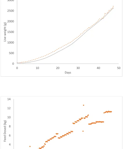
The performance of the trained DRNN model is given in table Table ??
211
Typical performance of the trained DRNN model is represented for one of the
212
remaining 12 test batches in Figure 1, which shows that the trained DRNN
213
was able to predict the bird weight satisfactorily even when the actual feed
214
intake was modulated by regular step changes. As with the broiler growth
215
model the pig growth DRNN model predicted the actual growth well, with an
216
average validation index γ2 = 0.9889, with γ2 = 1−P
(x−xmodel)2/P
x− 217
xmean)2.
218
3. Livestock Growth Control
219
In theory, using the identified DRNN model, many optimal control
prob-220
lems can be investigated, such as minimum time control, where feed intakes
221
are calculated such that animals can grow as fast as possible to reach the
0 500 1000 1500 2000 2500 3000
0 10 20 30 40 50
Li
ve
w
ei
gh
t
(g)
Days
0 2 4 6 8 10 12 14
0 10 20 30 40 50
Feed
Dosed
(kg
)
Days
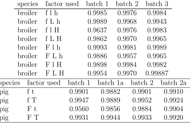
Table 1: The performance of the Differential Recurrent Neural Network models for broiler or pig growth for each of the data sets. Factors used are changes in feed, light, humidity and temperature indicated by F,L, H or T for the active state and f, l, h and t for the corresponding control or normal state.
species factor used batch 1 batch 2 batch 3
broiler f l h 0.9985 0.9976 0.9984
broiler f L h 0.9989 0.9968 0.9943
broiler f l H 0.9637 0.9976 0.9983
broiler f L H 0.9862 0.9970 0.9965
broiler F l h 0.9993 0.9981 0.9989
broiler F L h 0.9886 0.9957 0.9965
broiler F l H 0.9898 0.9984 0.9982
broiler F L H 0.9954 0.9970 0.99887
species factor used batch 1 batch 1a batch 2 batch 2a
pig f t 0.9901 0.9882 0.9901 0.9910
pig f T 0.9947 0.9889 0.9952 0.9924
pig F t 0.9560 0.9856 0.9884 0.9904
pig F T 0.9931 0.9944 0.9933 0.9920
target weight, and the minimum food problem, where optimal feed intake is
223
designed such that the total food consumption is minimized to achieve the
224
same target weight on the target day. However, due to the limited
experi-225
mental data, upon which the model was based, it would not be applicable to
226
some extreme situations, such as very low and high feed intakes. To ensure
227
the model was working within a reliable range that would not compromise
228
animal welfare, a regulation control problem was constructed to design
op-229
timal feed intake such that the actual animal growth followed a predesigned
230
curve smoothly with the minimum feed intake.
231
The above regulation problem was solved through a nonlinear model
pre-232
dictive control (NMPC) scheme. In the NMPC, at each sampling point, t0,
233
the average weight of an animal predicted by the model,x0 is compared with
234
the measured weight, xm. The difference, n =xm−x0 is treated as the
dis-235
turbance. This disturbance is assumed to be constant within the prediction
236
horizon, t0 ≤ t ≤ tf. Therefore, to correct the error caused by this
distur-237
bance, the actual set-point at a time point, t, within the prediction horizon
238
is biased as ˆx(t) = xr(t) +n, where xr(t) is the target weight. Then, the
239
optimal control problem to be solved at each sampling point, t0 is stated as
follows. 241 min u tf X
t=t0
α21(x(t)−xˆ(t))2+α22v2(t) +α32(∆v(t))2 (4)
s.t. x˙ =w5σ(w1x+w3u) +w6σ(w2x+w4u) (5)
x(t0) = x0 (6)
x(tf) = xf (7)
where,v2(t) =u(t) is the feed intake at dayt, ∆v(t) =v(t)−v(t−1), t0 and
242
tf are current and final days, respectively, x0 and xf are current and final
243
weights, respectively,α1,α2 and α3 are weights of the optimization problem
244
for weight accuracy, food consumption and smoothness respectively. Note
245
that although the optimal control problem in (4) is open loop, the correction
246
of modelling error, ˆx(t) =xr(t) +xm(t0)−x0 uses the real measured weight,
247
xm(t0), hence the actual control is feedback control.
248
The problem can be cast as a standard nonlinear least square problem,
249
minueTe, with residuals, e defined as follows. 250 e=
α1(x(t0+ 1)−xˆ(t0+ 1))
.. .
α1(x(tf)−xˆ(tf)) α2v(t0)
.. .
α2v(tf −1) α3∆v(t0)
.. .
α3∆v(tf −1)
(8)
The corresponding Jacobian, J =∂e/∂u can be derived through automatic
251
differentiation as explained by Al-Seyab & Cao (2008b). The optimal values
252
of v=v(t0), · · · , v(tf −1)
T
are then obtained iteratively using the LM
253
algorithm (Marquardt, 1963):
254
vk+1 = JTkJk+µI
−1
JTkek (9)
where ek and Jk are the residuals and the Jacobian corresponding to vk, µ
255
is a parameter adjusted by the algorithm to maintain a fast convergence.
Once the iteration had converged, the first instance of the obtained
opti-257
mal solution, vwas converted into the feed intake, u(t0) =v2(t0) and applied
258
to the real system. The whole procedure will be repeated at next sampling
259
time when a new measured average animal weight, xm is available.
260
4. Validation of the Growth Control Algorithm
261
To validate the control algorithm developed in the previous section, fresh
262
experiments were designed and carried out. In these experiments, new growth
263
curves were devised for the controller to attempt to follow as closely as
pos-264
sible by predicting the required feed intake. These new growth curves were
265
derived from the recommended (standard) growth curve for broilers provided
266
by Aviagen (2002), e.g. reaching a weight of 2.85 kg at 50 days of age and
267
the recoommneded growth curve for pigs PIC (2005), e.g. reaching a weight
268
of 92 kg at 21 weeks of age and were used for the development of the
con-269
troller. The broilers were grown according to the standard curve up to day
270
12 and from day 12 to 50 followed the new growth curves. The pigs were
271
grown according to the standard curve till week 6 and then followed the new
272
growth curves. The new growth curves for broilers were specified as,
273
• standard curve
274
• +12% of standard curve
275
• −12% of standard curve
276
• −12% to day 30 followed by +12% of standard curve (slow growth
277
followed by recovery growth)
278
and for pigs as
279
• standard curve
280
• alternating each 3 weeks between −20% and +20% of the standard
281
curve
282
The broiler growth controller was tested using four of the eight available
283
rooms. Each growth curve was tested with one room. Each room was initially
284
stocked with 265 day-old chicks (Ross 308). The pig growth controller was
285
tested using 8 pens in two rooms with the growth curves tested in paired
pens, each holding 10 pigs. Environmental conditions were kept identical to
287
the conditions used in the training and model validation trials, apart from the
288
frequency of light intensity change and number of meals fed daily for broilers
289
and room temperature for pigs. The total daily intake of each room or pen
290
was set by the controller. The controller was used for on-line calculation
291
of the feed intake, however with a 24-hour delay in implementation of the
292
calculated feed intake through a manual adjustment of the feed dosed.
293
The production results for broilers from the 4 batches and pigs from the
294
2 batches are summarised in Table 2 and Table 3, where the four controlled
295
(actual) weights at the end of the growth curve are compared with their
296
corresponding target values taken from the prescribed growth curves. The
297
predicted total feed intake was calculated from the sum of the controller–
298
predicted feed dosage rate. The actual total feed intake was calculated from
299
the sum of the feed dosed, corrected for the actual number of birds present.
300
The mean relative error and maximum deviation of the actual weights from
301
day 12–50 for broilers or week 6 to 21 for pigs were calculated as percentages,
302
where the mean relative error, ¯εand the maximum deviation,σmaxare defined
303
based on the actual weight,wact and the corresponding target weight, wth as
304
follows.
305
¯
ε = 1 39
P50
d=12
wact(d)−wth(d)
wth(d)
(10)
σmax = max12≤d≤50
wact(d)−wth(d)
wth(d)
(11)
Daily comparisons of controlled against modelled and standard growth
306
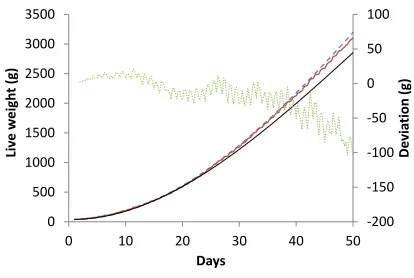
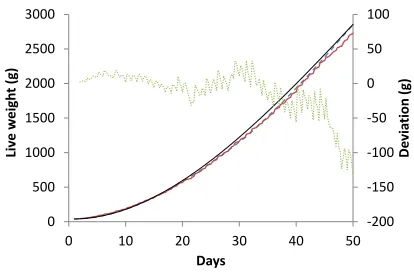
curves for broilers are shown in Figures 2 to 5 for the standard growth curve
307
and +12%, −12% and −12% followed by +12% of standard growth curves,
308
respectively.
309
The results for broilers clearly indicate that the controller is capable of
310
predicting the feed intake required to reach the end weight and follow the
311
reference growth curves well with an mean relative error less than 2%,
ex-312
cept for the −12% curve. The larger mean relative error in the−12% growth
313
curve was caused by a malfunction in the feeding equipment from day 16–19
314
(see Figure 6). Allthough the room recieved the correct feed amount for
315
each feeding period, due to blockages the feed was delivered to the birds
316
at very irregular intervals, potentially inhibiting growth (maximum
devia-317
tion from curve was −16%). However, the controller was able to return the
Table 2: Target live weight and achieved live weight of the broilers at age 50 days and goodness of fit of the achieved live weight compared to the set growth curve from day 12–50. Predicted and actual total feed intake per bird and feed conversion ratio (FCR) for the period of day 12–49. The standard growth curve had been derived from the optimal growth curve provided by Aviagen (2002).
Growth curve unit Standard +12% of −12% of −12% & +12%
standard standard of standard
Bird weight at 50 days
Target kg 2.85 3.20 2.51 2.85
Actual kg 2.73 3.10 2.44 2.72
Mean relative error % 1.8 1.8 2.8 1.6
Maximum deviation % 5.2 6.0 16.3 5.0
Total feed intake from day 12–49
Predicted kg.bird−1 4.66 4.99 4.30 4.62
Actual kg.bird−1 4.59 5.04 4.31 4.62
Feed conversion Ratio - 1.91 1.84 2.02 1.93
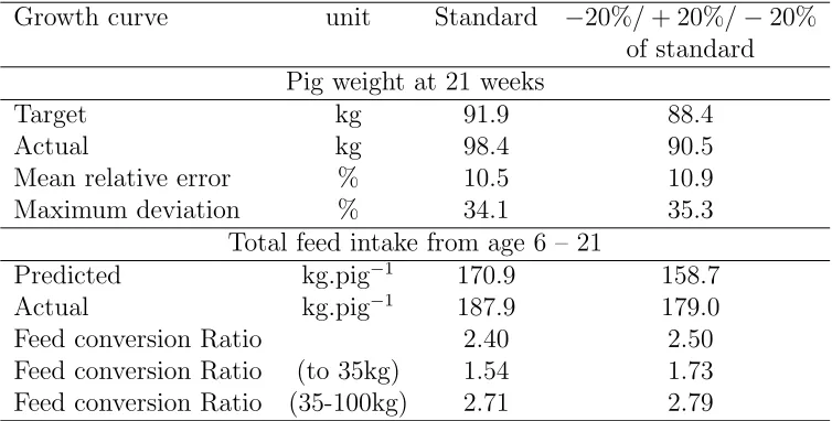
Table 3: Theoretical live weight and achieved live weight of the pigs at age 21 weeks and goodness of fit of the achieved live weight compared to the set growth curve from age 6 to 21 weeks. Predicted and actual total feed intake per bird and feed conversion ratio (FCR) for the period of week 6–21. The standard growth curve had been derived form the optimal growth curve provided by PIC (2005).
Growth curve unit Standard −20%/+ 20%/−20%
of standard Pig weight at 21 weeks
Target kg 91.9 88.4
Actual kg 98.4 90.5
Mean relative error % 10.5 10.9
Maximum deviation % 34.1 35.3
Total feed intake from age 6 – 21
Predicted kg.pig−1 170.9 158.7
Actual kg.pig−1 187.9 179.0
Feed conversion Ratio 2.40 2.50
Feed conversion Ratio (to 35kg) 1.54 1.73
-200 -150 -100 -50 0 50 100
0 500 1000 1500 2000 2500 3000 3500
0 10 20 30 40 50
De
via
ti
on
(g)
Liv
e
w
eigh
t
(g)
Days
Figure 2: The target standard (dashed line) and actual achieved (solid line) growth curves of broilers and the deviation of the target curve (dotted line, secondary axis).
-200 -150 -100 -50 0 50 100
0 500 1000 1500 2000 2500 3000 3500
0 10 20 30 40 50
De
via
ti
on
(g)
Liv
e
w
eigh
t
(g)
Days
-200 -150 -100 -50 0 50 100
0 500 1000 1500 2000 2500 3000
0 10 20 30 40 50
De
via
ti
on
(g)
Liv
e
w
eigh
t
(g)
Days
Figure 4: The target−12% below standard (dasehed line) and actual achieved (solid line) growth curves of broilers and the deviation of the target curve (dotted line, secondary axis). The standard growth curve (Aviagen) is plotted for comparison.
-200 -150 -100 -50 0 50 100
0 500 1000 1500 2000 2500 3000
0 10 20 30 40 50
De
via
ti
on
(g)
Liv
e
w
eigh
t
(g)
Days
growth to the set curve within 4 days, by feeding more than originally
an-319
ticipated. Excluding this period reduced the mean relative error to 1.9%.
320
Overall the mean relative error in this work is much lower than the 7–9%
321
reported by Cangar et al. (2008). The authors suggested that this high error
322
might be largely due to different conditions and systems for the weighing
323
and feed delivery used for generating data for creating and validating their
324
model (small scale, ”ideal” conditions) and for the validation of the control
325
algorithm (commercial conditions). In our work all steps were done on the
326
same scale, same conditions and with the same equipment. further more the
327
number of birds used in their trials was substantially higher, especially in the
328
commercial validation trials.
329
-100 -80 -60 -40 -20 0 20 40
0 200 400 600 800 1000 1200 1400
15 20 25
De
via
ti
on
(g)
Liv
e
w
eigh
t
(g)
Days
Figure 6: The target −12% below standard (dashed line) and actual achieved (solid line) growth curves of broilers and the deviation of the target curve (dotted line, secondary axis) for the period the feed system malfunctioned.
For all four broiler growth curves, the projected end weight was met
330
within small tolerances. From day 42 onwards the actual bird weight started
331
to deviate from the theoretical bird weight (slower growth). This could be
332
a undesirable feature of the DRNN model used. However, it also coincided
333
with the introduction of the withdrawal grower diet which in theory differs
334
in composition from the normal grower diet in the absence of coccidiostats
335
only. The absence of the coccidiostats should not affect the growth or feed
336
conversion, but it is not evident from the feed analysis if other minor changes
337
were made to the feed composition between the two deliveries that could have
338
affected the growth. In contrast to findings by Cangar et al. (2008) in these
trials the Ross 308 bird appeared to be capable of recovery growth (see Figure
340
5), i.e. the broilers were capable of regaining weight in excess of equivalent
341
growth by the standard growth curve beyond 31 days. One reason for this
342
difference is the lower energy and protein content of the diets used in this
343
work compared with current industry standards (approximately 15% lower).
344
The standard growth curve used was also set below the maximum potential
345
growth curve given by Aviagen (2002). Hence, the broilers were capable of
346
utilising the additional protein and energy provided as the maximum growth
347
potential had not yet been reached.
348
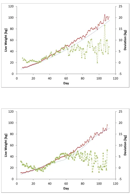
The growth controller for pigs equally indicates that the controller is
349
capable of predicting the feed intake to meet the desired growth curve and
350
end weight (see Figure 7). However, the mean relative error was significantly
351
higher at 10.5% and 10.9%, for the standard and recovery growth curves,
352
respectively. The larger mean relative error is potentially due to the lower
353
number of data sets available for determining the DRNN model parameters,
354
compared to the broiler DRNN model, 5 v 6, respectively, and the lower
355
number of changes in feed amount. Equally, the slower rate of growth meant
356
the dynamic changes in weight due to the changed feed intake reqime were
357
smaller compared to the broiler, potentially resulting in a less accurate model.
358
Creating even larger changes in the feed intake regime were however deemed
359
to be too detrimental for the pigs welfare. Another contributing factor is
360
the variation in temperature in the experimental conditions (standard versus
361
standard +7C). The effect of temperature on growth is well documented. Pigs
362
decrease their voluntary feed intake with increasing temperatures and hence
363
their average daily gain is lower (Hyun et al., 1998; Sutherland et al., 2006).
364
However, the FCR for the two temperature regimes was not significantly
365
different as was expected (Sutherland et al., 2006).
366
The DRNN model used in the controller controlled not only the daily
367
feed intake on line, but predicted accurately the required feed intake for the
368
whole of the growing period. This novel addition will be very useful to
farm-369
ers when deciding on a growth curve suitable for various scenarios. From the
370
four broiler growth curves used in this trial the +12% of standard growth
371
curve is better from an economic point of view, as it has by far the lowest feed
372
conversion ratio (FCR). The authors suggest this is largely due to making
373
better use of the genetic potential of the broilers. Using the slow growth with
374
recovery growth option, has potential advantages for animal welfare in terms
375
of leg health and proved to be no worse in achieving the final weight with
376
a similar FCR and total feed intake requirement, compared to the standard
growth curve. The FCR’s achieved here are however significantly higher
378
than those commonly achieved on commercial farms, where the best
pro-379
ducers achieve 1.6 -1.7 FCR, approximately. The purposely lower protein
380
content of the feed used in these trials, approximately 15% less, appears to
381
be the root cause of the poorer FCR. The otherwise optimal
environmen-382
tal conditions had no negative effect on the FCR. Using optimal diets for
383
the genetic growth potential might reduce the effectiveness of the model to
384
recover lost growth over a number of days as shown in this work, as the
385
maximum daily weight gain had already been reached (Cangar et al., 2008).
386
The feed conversion ratio for pigs in these trials and expecially the for the
387
standard growth curve which had the best performance in economic terms,
388
compares favourably to the industry average of 2.35 reported by BPEX
389
(2011, 2015) for rearer/finisher pigs combined (8-100 kg), as well as the
indi-390
vidual FCR’s for rearer and finisher at 1.71 and 2.67, respectively, despite the
391
suboptimal lower protein content of the feed used in these trials. The optimal
392
environmental conditions in the new animal welfare facility and therefor the
393
significant reduction in disease burden on the pigs will have contributed to
394
the good growth performance.
395
5. Conclusions
396
An accurate differential recurrent neural network model of broiler and pig
397
growth has been identified, validated and tested successfully. The DRNN
398
model accurately described the dynamic time variable growth of housed
live-399
stock. Typically the mean square error and standard deviation between the
400
broiler growth model and data were of the order of 0.02 and 0.03, respectively
401
and the equivalent figures for the pig growth model were of the order of 0.02
402
and 0.05, respectively.
403
The nonlinear model predictive controller, incorporating the DRNN model,
404
was constructed to predict the feed quantity required for the broilers to grow
405
following predetermined growth curves. The NMPC accurately predicted the
406
feed quantity to achieve a range of predetermined growth curves. The mean
407
relative error for the period from day 12–50 was 1.8% for broilers and for pigs
408
10.5% for the period from 6 to 21 weeks. The NMPC was capable of
accu-409
rately predicting compensatory growth rates following two days of retarded
410
growth rates due to feeding equipment failure. In addition, the controller was
411
able to predict the total feed intake for the whole growth period accurately.
6. Acknowledgement
413
This work was funded by the Biotechnology and Biological Sciences
Re-414
search Council (BBC518922/1) and approved by the Clinical Research
Eth-415
ical Review Board (CRERB) of the Royal Veterinary College. The authors
416
would like to thank the staff of the Biological Services Unit for providing
417
excellent stockmen during the trials.
418
7. Bibliography
419
Aerts, J., Buggenhout, S. V., Vranken, E., Lippens, M., Buyse, J.,
De-420
cuypere, E., & Berckmans, D. (2003a). Active control of the growth
trajec-421
tory of broiler chickens based on online animal responses. Poultry Science,
422
82, 1853–1862.
423
Aerts, J., Lippens, M., Groote, G. D., Buyse, J., Decuypere, E., Vranken, E.,
424
& Berckmans, D. (2003b). Recursive prediction of broiler growth response
425
to feed intake by using a time-variant parameter estimation method.
Poul-426
try Science,82, 40–49.
427
Ahmadi, H., & Mottaghitalab, M. (2007). Hyperbolastic models as a new
428
powerful tool to describe broiler growth kinetics. Poultry Science, 86,
429
2461–2465.
430
Ahmadi, H., & Mottaghitalab, M. (2008). Predicting performance of broiler
431
chickens from dietary nutrients using group method of data handling-type
432
neural networks. British Poultry Science, 49, 315–320.
433
Al-Seyab, R., & Cao, Y. (2008a). Differential recurrent neural network based
434
predictive control. Computers and Chemical Engineering,32, 1533–1545.
435
Al-Seyab, R., & Cao, Y. (2008b). Nonlinear system identification for
predic-436
tive control using continuous time recurrent neural networks and automatic
437
differentiation. Journal of Process Control, 18, 568–581.
438
Aviagen (2002). Broiler management manual.. Aviagen Ltd, Newbridge,
439
Midlothian, Scotland, UK.
440
Black, J. (2014). Brief history and future of animal simulation models for
441
science and application. Animal production science, 54, 1883–1895.
BPEX (2011). Improving key performance
indica-443
tiors: Rearing herd. action for productivity 25. URL:
444
http://pork.ahdb.org.uk/media/2111/Action-25-Rearing-herd.pdf.
445
BPEX (2015). The BPEX Yearbook 2014-2015.. AHDB Pork, Agriculture
446
and Horticulture Development Board, Kenilworth, United Kingdom.
447
Butterworth, A., & Arnould, D. (2009). Standardisation of measures of
448
broiler lameness. In B. Forkman, & L. Keeling (Eds.), Assessment of
449
Animal Welfare Measures for Layers and Broilers. number 9 in Welfare
450
Quality Reports (pp. 31–39). Cardiff, UK: Cardiff University.
451
Cangar, O., Aerts, J.-M., Vranken, E., & Berckmans, D. (2008). Effects of
452
different target trajectories on the broiler performance in growth control.
453
Poultry Science, 87, 2196–2207.
454
Cao, Y. (2005). A formulation of nonlinear model predictive control using
455
automatic differentiation. Journal of Process Control, 15, 851–858.
456
Charles, D., & Walker, A. (2002). Poultry Environment Problems. A guide
457
to solutions.. Nottingham University Press, Nottingham, UK.
458
Demmers, T., Cao, Y., Gauss, S., Lowe, J., Parsons, D., & Wathes, C.
459
(2010). Neural predictive control of broiler chicken growth. In J. R.
460
Banga, P. Bogaerts, J. V. Impe, D.Dochain, & I. Smets (Eds.),11th IFAC
461
Symposium on Computer Applications in Biotechnology. Leuven, Belgium
462
IFAC-PapersOnLine 11:6. doi:10.3182/20100707-3-BE-2012.0061.
463
Doeschl-Wilson, A. B., Whittemore, C. T., Knap, P. W., & Schofield, C. P.
464
(2004). Using visual image analysis to describe pig growth in terms of size
465
and shape. Animal Science, 79, 415–427.
466
Emmans, G. (1995). Problems in modeling the growth of poultry. Worlds
467
Poultry Science Journal,51, 77–89.
468
Frost, A., Parsons, D., Stacey, K., Robertson, A., Welch, S., Filmer, D., &
469
Fothergill, A. (2003). Progress towards the development of an integrated
470
management system for broiler chicken production. Computers and
Elec-471
tronics in Agriculture,39, 227–240.
Frost, A., Schofield, C., Beaulah, S., Mottram, T., Lines, J., & Wathes,
473
C. (1997). A review of livestock monitoring and the need for integrated
474
systems. Computers and Electronics in Agriculture, 17, 139–159.
475
Gous, R., Moran, E., Stilborn, H., Bradford, G., & Emmans, G. (1999).
476
Evaluation of the parameters needed to describe the overall growth, the
477
chemical growth, and the growth of feathers and breast muscles of broilers.
478
Poultry Science, 78, 812–821.
479
Hyun, Y., Ellis, M., Riskowski, G., & Johnson, R. W. (1998). Growth
per-480
formance of pigs subjected to multiple concurrent environmental stressors.
481
Journal of Animal Science,76, 721–727.
482
Kyriazakis, I., & Whittemore, C. (2006). Whittemore’s science and proactice
483
of pig production. Blackwell Publishers,Oxford, UK.
484
Marquardt, D. (1963). An algorithm for least-squares estimation of nonlinear
485
parameters. SIAM Journal of Applied Mathematics, 11, 431–441.
486
Parsons, D. J., Green, D. M., Schofield, C. P., & Whittemore, C. T. (2007).
487
Real-time control of pig growth through an integrated management system.
488
Biosystems Engineering,96, 257–266.
489
PIC (2005). Wean to Finish Manual. PIC UK Ltd, Stapeley, Nantwich, UK.
490
Schofield, C. P., Marchant, J. A., White, R. P., Brandl, N., & Wilson, M.
491
(1999). Monitoring pig growth using a prototype imaging system. Journal
492
of Agricultural Engineering Research, 72, 205–210.
493
Scott, K., J.Chennells, D., Armstrong, D., L.Taylor, P.Gill, B., & Edwards,
494
S. A. (2007). The welfare of finishing pigs under different housing and
495
feeding systems: liquid versus dry feeding in fully-slatted and straw-based
496
housing. Animal Welfare, 16, 53–62.
497
Stacey, K., Parsons, D., Frost, A., Fisher, C., Filmer, D., & Fothergill, A.
498
(2004). An automatic growth and nutrition control system for broiler
499
production. Biosystems Engineering,89, 363–371.
500
Sutherland, M. A., Niekamp, S. R., Rodriguez-Zas, S. L., & Salak-Johnson,
501
J. L. (2006). Impacts of chronic stress and social status on various
physi-502
ological and performance measures in pigs of different breeds. Journal of
503
Animal Science,84, 588–596.
Wathes, C., Kristensen, H., Aerts, J.-M., & Berckmans, D. (2008). Is
preci-505
sion livestock farming an engineer’s daydream or nightmare, an animal’s
506
friend or foe, and a farmer’s panacea or pitfall? Computers and electronics
507
in agriculture, 64, 2–10.
-5 0 5 10 15 20 25
0 20 40 60 80 100 120
0 20 40 60 80 100 120
De
via
tion (k
g)
Liv
e
W
eigh
t [kg]
Day
-5 0 5 10 15 20 25
0 20 40 60 80 100 120
0 20 40 60 80 100 120
De
via
tion [
kg]
Liv
e
W
eigh
t [kg]
Day