A Machine Learning approach to 5G Infrastructure Market optimization

A Machine Learning approach to 5G

Infrastructure Market optimization

Dario Bega, Marco Gramaglia, Albert Banchs,

Senior Member, IEEE,

Vincenzo

Sciancalepore

Member, IEEE,

Xavier Costa-P ´erez,

Senior Member, IEEE

Abstract—It is now commonly agreed that future 5G Networks will build upon the network slicing concept. The ability to provide virtual, logically independent “slices” of the network will also have an impact on the models that will sustain the business ecosystem. Network slicing will open the door to new players: the infrastructure provider, which is the owner of the infrastructure, and the tenants, which may acquire a network slice from the infrastructure provider to deliver a specific service to their customers. In this new context, how to correctly handle resource allocation among tenants and how to maximize the monetization of the infrastructure become fundamental problems that need to be solved. In this paper, we address this issue by designing a network slice admission control algorithm that (i) autonomously learns the best acceptance policy while (ii) it ensures that the service guarantees provided to tenants are always satisfied. The contributions of this paper include: (i) an analytical model for the admissibility region of a network slicing-capable 5G Network, (ii) the analysis of the system (modeled as a Semi-Markov Decision Process) and the optimization of the infrastructure providers revenue, and (iii) the design of a machine learning algorithm that can be deployed in practical settings and achieves close to optimal performance.

Index Terms—Network Slicing, Admission Control, Neural Networks, Machine Learning, 5G Networks

F

1

I

NTRODUCTION

T

HEexpectations that build around future 5G Networks are

very high, as the envisioned Key Performance Indicators (KPIs) represent a giant leap when compared to the legacy 4G/LTE networks. Very high data rates, extensive coverage, sub-ms delays are just few of the performance metrics that 5G networks are expected to boost when deployed.

This game changer relies on new technical enablers such as Software-Defined Networking (SDN) or Network Function Virtualization (NFV) that will bring the network architecture

from a purely hardbox based paradigm (e.g., a eNodeB or a

Packet Gateway) to a completelycloudifiedapproach, in which

network functions that formerly were hardware-based (e.g., baseband processing, mobility management) are implemented as software Virtual Network Functions (VNFs) running on a,

possibly hierarchical, general purpose telco-cloud.

Building on these enablers, several novel key concepts have been proposed for next generation 5G networks [1]; out of

those, Network Slicing [2] is probably the most important

one. Indeed, there is a wide consensus in that accommodating

• D. Bega and A. Banchs are with the IMDEA Networks Institute, 28918 Legan´es, Spain, and also with the Telematic Engineering De-partment, University Carlos III of Madrid, 28911 Legan´es, Spain (e-mail:[email protected]; [email protected]).

• M. Gramaglia is with the Telematic Engineering Department, Uni-versity Carlos III of Madrid, 28911 Legan´es, Spain(e-mail: [email protected]).

• V. Sciancalepore and X. Costa-P´erez are with NEC Laboratories Europe, 69115 Heidelberg, Germany (e-mail: [email protected]).

Manuscript received April 25, 2018; revised June 27, 2018 and November 27, 2018; accepted January 25, 2019. Date of publication xxxx xx, xxxx; date of current version xxxx xx, xxxx. (Corresponding author: Dario Bega.) For information on obtaining reprints of this article, please send e-mail to: [email protected], and reference the Digital Object Identifier below. Digital Object Identifier no. xx.xxxx/TMC.xxxx.xxxxxxx

the very diverse requirements demanded by 5G services using the same infrastructure will not be possible with the current, relatively monolithic architecture in a cost efficient way. In contrast, with network slicing the infrastructure can be divided in different slices, each of which can be tailored to meet specific service requirements.

A network slice consists of a set of VNFs that run on a virtual network infrastructure and provide a specific telecom-munication service. The services provided are usually typified in macro-categories, depending on the most important KPIs they target. Enhanced Mobile Broadband (eMBB), massive Machine Type Communication (mMTC) or Ultra Reliable Low Latency Communication (URLLC) are the type of services

currently envisioned by,e.g., ITU [3]. Each of these services

is instantiated in a specific network slice, which has especially tailored management and orchestration algorithms to perform the lifecycle management within the slice.

In this way, heterogeneous services may be provided using the same infrastructure, as different telecommunication ser-vices (that are mapped to a specific slice) can be configured independently according to their specific requirements.

Addi-tionally, thecloudificationof the network allows for the

cost-efficient customization of network slices, as the slices run on a shared infrastructure.

Network Slicing enables a new business model around mobile networks, involving new entities and opening up new business opportunities. The new model impacts all the players of the mobile network ecosystem. For end-users, the capability of supporting extreme network requirements [3] enables new services that could not be satisfied with current technologies, providing a quality of experience beyond that of todays networks. For tenants such as service providers, network slicing allows to tailor the network service to the specific 0000–0000 c_⃝2019 IEEE. Personal use is permitted, but republication/redistribution requires IEEE permission.

needs of the service being provided, adjusting the slice’s operation to the service provider’s needs. For mobile network operators, network slicing allows to target new customers with specific service requirements, such as industrial sectors with stringent requirements, ultimately providing new revenue streams coming from the new customers.

This business model underlying network slicing is the Infrastructure as a Service (IaaS), which is expected to increase the number of available revenue streams in 5G. This model has already been successfully applied to the cloud computing infrastructure by providers such as Amazon AWS or Microsoft Azure. However, cloud computing platforms are selling to

customers (i.e., tenants) cloud resources (e.g., CPU, memory,

storage) only, while in a 5G Infrastructure market such as the one enabled by network slicing, the traded goods also include

network resources (e.g., spectrum, transport network). This

entails a totally different problem due to the following reasons:

(i) spectrum is a scarce resource for which over-provisioning

is not possible, (ii) the actual capacity of the systems (i.e.,

the resources that can actually be sold) heavily depends

on the mobility patterns of the users, and (iii) the Service

Level Agreements (SLAs) with network slices tenants usually impose stringent requirements on the Quality of Experience (QoE) perceived by their users. Therefore, in contrast to IaaS, in our case applying a strategy where all the requests coming to the infrastructure provider are admitted is simply not possible. The ultimate goal of InPs is to obtain the highest possible profit from of the deployed infrastructure, thus maximizing monetization. The design of a network slice admission control policy that achieves such goal in this spectrum market is still an open problem. More specifically, the network capacity bro-ker algorithm that has to decide on whether to admit or reject new network slice requests shall simultaneously satisfy two

different goals: (i) meeting the service guarantees requested by

the network slices admitted while (ii) maximizing the revenue

of a network infrastructure provider.

The goal of meeting the desired service guarantees needs to consider radio related aspects, as a congested network will likely not be able to meet the service required by a network slice. Conversely, the goal of maximizing the revenue obtained by the admission control should be met by applying an on-demand algorithm that updates the policies as long as new requests arrive.

In this paper, we propose a Machine Learning approach to the 5G Infrastructure Market optimization. More specifically,

the contributions of this paper are: (i) we provide an analytical

model for the admissibility region in a sliced network, that provide formal service guarantees to network slices, and

(ii) we design an online Machine Learning based admission

control algorithm that maximizes the monetization of the infrastructure provider.

Machine learning is the natural tool to address such a complex problem. As discussed in detail along the paper, this problem is highly dimensional (growing linearly with the number of network slices classes) with a potentially huge number of states (increasing exponentially with the number of classes) and many variables (one for each state). Furthermore, in many cases the behavior of the tenants that request slices is

not knowna prioriand may vary with time. For these reasons,

traditional solutions building on optimization techniques are not affordable (because of complexity reasons) or simply im-possible (when slice behavior is not known). Instead, machine learning provides a mean to cope with such complex problems while learning the slice behavior on the fly, and thus allows to develop a practical approach to deal with such a complex and potentially unknown system.

The rest of the paper is structured at follows. In Section 2 we review the relevant works related to this paper in the fields of resource allocation for network slicing aware net-works, network slice admission control and machine learning applied to 5G Networks. In Section 3 we describe our System Model, while the analytical formulation for the network slice admissibility region is provided in Section 4. In Section 5 we model the decision-making process by means of a Markovian analysis, and derive the optimal policy which we use as a benchmark. In Section 6 we present a Neural Networks approach based on deep reinforcement learning, which pro-vides a practical and scalable solution with close to optimal performance. Finally, in Section 7 we evaluate the proposed algorithm in a number of scenarios to assess its performance in terms of optimality, scalability and adaptability to different conditions, before concluding the paper in Section 8.

2

S

TATE OF THE ART

While the network slicing concept has only been proposed recently [2], it has already attracted substantial attention. 3GPP has started working on the definition of requirements for network slicing and the design of a novel network architecture for supporting it [4], whereas the Next Generation Mobile Networks Alliance (NGMN) identified network sharing among slices (the focus of this paper) as one of the key issues to be addressed [5]. While there is a body of work on the literature on spectrum sharing [6]–[9], these proposal are not tailored to the specific requirements of the 5G ecosystem. Conversely, most of the work has focused on architectural aspects [10], [11] with only a limited focus on resource allocation algorithms. In [12], the authors provide an analysis of network slicing admission control and propose a learning algorithm; however, the proposed algorithm relies on an offline approach, which is not suitable for a continuously varying environment such as the 5G Infrastructure market. Moreover, the aim is to maximize the overall network utilization, in contrast to our goal here which is focused on maximizing InP revenues.

knowledge of arriving requests statistics, thus making it im-practicable in real scenarios. Another work in this field is the one of [14], with similar limitations.

Learning algorithms are in the spotlight since Mnith et al. [16] designed a deep learning algorithm called “deep Q-network” to deal with Atari games, and further improved it in [17] making the algorithm able to learn successful policies directly from high-dimensional sensory inputs and reach human-levels performance in most of Atari games. Another approach is “AlphaGo”, which builds on deep neural networks to play with the “Go” game [18]. Many more algorithms have been proposed [19]–[23], which are mostly applied in games, robotics, natural language processing, image recognition problems.

The application of Reinforcement and Machine learning approaches to mobile networks is also gaining popularity. To name a few examples, the work in [24] proposes a Q-learning algorithm for improving the reliability of a millimeter wave (mmW) non-line-of-sight small cell backhaul system, while in [25] Q-learning is implemented to solve the adaptive call admission control problem.

Machine learning has been applied to a wide span of applications in 5G networks, ranging from channel estima-tion/detection for massive MIMO channel to user behav-ior analysis, location prediction or intrusion/anomaly detec-tion [26]. For instance, decision tree and informadetec-tion-theoretic regression models have been used in [27] in order to identify radio access networks problems. The authors of [28] em-ploy a deep learning approach for modulation classification, which achieves competitive accuracy with respect to traditional schemes. The authors of [29] apply deep neural networks to approximate optimization algorithm for wireless networks resources management.

This work is an extension of the paper in [30]. In that paper, the problem of slice admission control for revenue maximization was addressed by employing Q-learning. While this provides the ability to adapt to changing environments while achieving close to optimal performance, an inherent drawback of Q-learning is its lack of scalability, as the learning time grows excessively when the state space becomes too large. In contrast, the algorithm proposed in this paper is based on Neural Networks, and it is shown to scale with the size of the network, quickly converging to optimal performance.

To the best of our knowledge, the work presented in this paper along with the previous version in [30] are the first ones that build on Machine Learning to address the problem of admission control for a 5G Infrastructure Market, with the aim of maximizing the InP’s revenue while guaranteeing the SLAs of the admitted slices.

3

S

YSTEM

M

ODEL

As discussed in Section 1, 5G networks necessarily introduce changes in the applied business models. With the legacy and rather monolithic network architecture, the main service offered is a generic voice and best-effort mobile broadband. Conversely, the high customizability that 5G Networks intro-duce will enable a richer ecosystem on both the portfolio of

available services and the possible business relationships. New players are expected to join the 5G market, leading to an

ecosystem that is composed of (i) users that are subscribed

to a given service provided by a (ii) tenant that, in turn,

uses the resources (i.e., cloud, spectrum) provided by an (iii)

infrastructure provider.1 _{In the remainder of the paper we use}

this high level business model as basis for our analysis. In the following, we describe in details the various aspects related to our system model.

Players.As mentioned before, in our system model there are

the following players: (i) the Infrastructure Provider, InP,

who is the owner of the network (including the antenna location and cloud infrastructure) and provides the tenants with network slices corresponding to a certain fraction of

network resources, (ii) the tenants, which issue requests to

the infrastructure provider to acquire network resources, and use these resources to serve their users, providing them a

specific telecommunication service, and finally (iii) the

end-users, which are subscribers of the service provided by a tenant which uses the resources of the infrastructure provider.

Network model. The ecosystem described above does not

make any distinction on the kind of resources an InP may provide to the tenants. From the various types of resources, spectrum will typically be the most important factor when taking a decision on whether to accept a request from a tenant. Indeed, cloud resources are easier to provision, while increasing the spectrum capacity is more complex and more expensive (involving an increase on antenna densification). Based on this, in this paper we focus on the wireless access network as the most limiting factor. In our model of the

wireless access, the network has a set of base stationsBowned

by an infrastructure provider. For each base stationb∈ B, we

let Cb denote the base station capacity. We further refer to

the system capacity as the sum of the capacity of all base

stations,C=∑_BCb. We letU denote the set of users in the

network.2 _{We consider that each user u ∈ U in the system}

is associated to one base station b ∈ B. We denote by fub

the fraction of the resources of base station b assigned to

user u, leading to a throughput for user u of ru = fubCb.

We also assume that users are distributed among base stations according to a given probability distribution; we denote by

Pu,bthe probability that useruis associated with base station

b. We assume that these are independent probabilities, i.e.,

each user behaves independently from the others.

Traffic model. 5G Networks provide diverse services which

are mapped to three different usage scenarios or slice cat-egories: eMBB, mMTC and URLLC [3]. As the main bot-tleneck from a resource infrastructure market point of view is spectrum, different slice categories need to be matched based to their requirements in terms of the spectrum usage. For instance eMBB-alike slices have a higher flexibility with respect to resource usage, and can use the leftover capacity of URLLC services which have more stringent requirements on

1. While some of these roles may be further divided into more refined ones, as suggested in [31], the ecosystem adopted in this paper reflects a large consensus on the current view of 5G networks.

the needed capacity.

Following the above, in this paper we focus on elastic and inelastic traffic as it is the main distinguishing factor for spectrum usage and thus provides a fairly large level of generality. In line with previous work in the literature [32], we consider that inelastic users require a certain fixed throughput

demand which needs to be satisfied at all times,3 in contrast

to elastic users which only need guarantees on the average

throughput, requiring that the expected average throughput over long time scales is above a certain threshold. That is, for inelastic users throughput needs to be always (or with a very high probability) above the guaranteed rate, while the throughput for elastic users is allowed to fall below the guaranteed rate during some periods as long as the average stays above this value.

We let I denote the set of classes of inelastic users; each

classi∈ Ihas a different rate guaranteeRiwhich needs to be

satisfied with a very high probability; we refer the probability that this rate is not met as the outage probability, and impose

that it cannot exceedP¯out, which is set to a very small value.

We further letNidenote the number of inelastic users of class

i ∈ I, and Pi,b be the probability that a user of class i is at

base station b. Finally, we let Ne be the number of elastic

users in the network and Re their average rate guarantee.

At any given point in time, the resources of each base stations are distributed among associated users as follows:

inelastic users u ∈ I are provided sufficient resources to

guaranteeru=Ri, while the remaining resources are equally

shared among the elastic users. In case there are not sufficient resources to satisfy the requirements of inelastic users, even when leaving elastic users with no throughput, we reject as many inelastic users as needed to satisfy the required throughput guarantees of the remaining ones.

Note that the above traffic types are well aligned with the slice categories defined in 3GPP, as the elastic traffic behavior is in line with the eMBB and mMTC services, while inelastic behavior matches the requirements of URLCC services.

Network slice model.By applying the network slicing concept

discussed in Section 1, the network is divided into different logical slices, each of them belonging to one tenant. Thus, we

characterize a network slice by (i) its traffic type (elastic or

inelastic), and (ii) its number of users (i.e., the subscribers of

a given service) that have to be served.

A network slice comes with certain guarantees provided by an SLA agreement between the tenant and the infrastructure provider. In our model, a tenant requests a network slice that comprises a certain number of users and a traffic type. Then, as long as the number of users belonging to a network slice is less or equal than the one included in the SLA agreement, each of them will be provided with the service guarantees corresponding to their traffic type.

A network slice may be limited to a certain geographical area, in which case the corresponding guarantees only apply

3. Note that, by ensuring that the instantaneous throughput of inelastic traf-fic stays above a certain threshold, it is possible to provide delay guarantees. Indeed, as long as the traffic generated by inelastic users is not excessive, by providing a committed instantaneous throughput we can ensure that queuing delays are sufficiently low.

to the users residing in the region. In our model, we focus on the general case and consider network slices that span over the entire network. However, the model could be easily extended to consider restricted geographical areas.

Following state of the art approaches [11], network slicing onboarding is an automated process that involves little or no human interaction between the infrastructure provider. Based on these approaches, we consider a bidding system in order to dynamically allocate network slices to tenants. With this,

tenants submit requests for network slices (i.e., a certain

number of users of a given service) to the infrastructure provider, which accepts or rejects the request according to an admission control algorithm such as the one we propose in this paper. To that aim, we characterize slices request by:

• Network slice duration t: this is the length of the time

interval for which the network slice is requested.

• Traffic typeκ: according to the traffic model above, the

traffic type of a slice can either be elastic or inelastic traffic.

• Network slice size N: the size of the network slice

is given by the number of users it should be able to accommodate.

• Price ρ: the cost a tenant has to pay for acquiring

resources for a network slice. The price is per time unit, and hence the total revenue obtained by accepting a

network slice is given byr=ρt.

Following the above characterization, an infrastructure provider will have catalogs of network slice blueprinted by

predefined values for the tuple {κ, N, ρ}, which we refer to

as network slice classes. Tenants issue requests for one of the slice classes available in the catalogue, indicating the total

duration t of the network slice. When receiving a request,

an infrastructure provider has two possible decisions: it can reject the network slice and the associate revenue to keep the resources free or it can accept the network slice and charge the

tenantrdollars. If accepted, the infrastructure provider grants

resources to a tenant during at-window.

To compute the profit received by the tenant, we count the aggregated revenue resulting from all the admitted slices. This

reflects the net benefit of the InP as long as (i) the costs of

the InP are fixed, or (ii) they are proportional to the network

utilization (in the latter case,ρreflects the difference between

the revenue and cost of instantiating a slice). We argue that this covers a wide range of cases of practical interest such as spectrum resources or computational ones. Moreover, in the cases where costs are not linear with the network usage, our analysis and algorithm could be extended to deal with such cases by subtracting the cost at a given state from the revenue.

4

B

OUNDING THE ADMISSIBILITY REGION

theadmissibility region,i.e., the maximum number of network slices that can be admitted in the system while guaranteeing that the SLAs are met for all tenants. Indeed, if admitting a new network slice in the system would lead to violating the SLA of already admitted slices, then such a request should be rejected. In the following, we provide an analysis to determine

the admissibility region, denoted byA, as a first step towards

the design of the optimal admission algorithm.

4.1 Admissibility region analysis

We say that a given combination of inelastic users of the various classes and elastic users belongs to the admissibility

region, i.e., {N1, . . . , N_|I|, Ne} ∈ A, when the guarantees

described in the previous section for elastic and inelastic traffic are satisfied for this combination of users. In the following,

we compute the admissibility region A.

In order to determine whether a given combination of

users of different types,{N1, . . . , N|I|, Ne}, belongs toA, we

proceed as follows. We first compute the outage probability

for an inelastic user of class i ∈ I, Pout,i. Let Rb be the

throughput consumed by the inelastic users atb. The average

value ofRb can be computed as

E[Rb] =

∑

j∈I

NjPj,bRj, (1)

and the typical deviation as

σ2_b =∑

j∈I

Njσ2j,b, (2)

whereσ2

j,bis the variance of the throughput consumed by one

inelastic user of class j, which is given by

σ_j,b2 =Pj,b(Rj−Pj,bRj)2+ (1−Pj,b)(Pj,bRj)2

=Pj,b(1−Pj,b)R2j. (3)

Our key assumption is to approximate the distribution of

the committed throughput at base station b by a normal

distribution of mean Rb and variance σb2, i.e., N(E[Rb], σb2).

Note that, according to [33], this approximation is appropriate as long as the number of users per base station in the boundary of the admissibility region is no lower than 5, which is generally satisfied by cellular networks (even in the extreme case of small cells).

The outage probability at base station b is given by the

probability that the committed throughput exceeds the base station capacity, i.e.,

Pout,b=P(Rb> Cb), (4)

whereCb be the capacity of base stationb.

To compute the above probability with the normal approx-imation, we proceed as follows:

Pout,b≈1−Φ

(

Cb+ ˜Cb−E[Rb,i]

σb,i

)

, (5)

where Φ(·) is the cumulative distribution function of the

standard normal distribution andC˜b is a continuity correction

factor that accounts for the fact Rb is not a continuous

variable. In line with [34], where this is applied to a binomial distribution and the correction factor is one half of the step size, in our case we a set the continuity correction factor as one half of the average step size, which yields

˜

Cb=

1 2

∑

j_∈IPj,bNjRj

∑

j∈IPj,bNj

. (6)

Once we have obtained Pout,b, we compute the outage

probability of an inelastic user of class i with the following

expression:

Pout,i=

∑

b_∈B

Pi,bPout,b. (7)

Next, we compute the average throughput of an elastic user.

To this end, we assume that (i) in line with [32], elastic users

consume all the capacity left over by inelastic traffic, (ii) there

is always at least one elastic user in each base station, and (iii)

all elastic users receive the same throughput on average. With the above assumptions, we proceed as follows. The average committed throughput consumed by inelastic users at

base stationbis given by

E[Rb] =

∑

i∈I

NiPi,bRi, (8)

which gives an average capacity left over by inelastic users

equal toCb−E[Rb]. This capacity is entirely used by elastic

users as long as the base station is not empty. The total capacity usage by elastic users is then given by the sum of this term over all base stations. As this capacity is equally shared (on average) among all elastic users, this leads to the following expression for the average throughput of an elastic user:

re=

∑

b∈BCb−E[Rb]

Ne

. (9)

Based on the above, we compute the admissibility regionA

as follows. For a given number of inelastic users in each class,

Ni, i∈ I, and of elastic users, Ne, we compute the outage

probability of the inelastic classes, Pout,i, and the average

throughput of the elastic users,re. If the resulting values meet

the requirements for all classes, i.e., Pout,i ≤ P¯out ∀i and

re≥Re, then this point belongs to the admissibility region,

and otherwise it does not.

4.2 Validation of the admissibility region

In order to assess the accuracy of the above analysis, we compare the admissibility region obtained theoretically against the one resulting from simulations. To this end, we consider the reference scenario recommended by ITU-T [35], which

consists of |B|= 19 base stations placed at a fixed distance

of 200m. Following the system model of Section 3, we have elastic and inelastic users. All inelastic users belong to the same class, and all users (elastic and inelastic) move in the area covered by these base stations following the Random Waypoint (RWP) mobility model, with a speed uniformly distributed between 2 and 3 m/s.

The association procedure of elastic and inelastic users with base stations is as follows. Inelastic users try to associate to

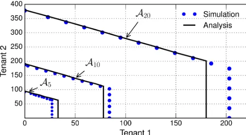
Fig. 1: Admissibility region: analysis vs. simulation. Otherwise they do not associate and generate an outage event, joining again the network when their throughput guarantee can be satisfied. When associating, they consume a capacity

Ri from the base station. The probability of association to

each base station (i.e., thePi,b values) are extracted from the

simulations and fed into the analysis.

Similarly to inelastic users, elastic users always associate to the nearest base station. All the elastic users associated to a base station fairly share among them the capacity left over by inelastic users. Upon any association event, the throughput received by the users associated to the new and the old base station changes accordingly.

Following the above procedure, we have simulated all the

possible combinations of inelastic and elastic users,{Ni, Ne}.

For each combination, we have evaluated the average through-put received by elastic users, comthrough-puted over samples of 10

seconds time windows, and the outage probability Pout of

inelastic users, computed as the fraction of time over which they do not enjoy their guaranteed throughput. If these two metrics (average elastic traffic throughput and inelastic traffic outage probability) are within the guarantees defined for the two traffic types, we place this combination inside the admissibility region, and otherwise we place it outside.

Fig. 1 shows the boundaries of the admissibility region obtained analytically and via simulation, respectively, for different throughput guarantees for elastic and inelastic users

(A5 : Ri = Re = Cb/5, A10 : Ri = Re = Cb/10 and

A20 : Ri = Re = Cb/20) and P¯out = 0.01. We observe

that simulation results follow the analytical ones fairly closely. While in some cases the analysis is slightly conservative in the admission of inelastic users, this serves to ensure that inelastic users’ requirements in terms of outage probability are always met.

5

M

ARKOVIAN

M

ODEL FOR THE DECISION

-MAKING PROCESS

While the admissibility region computed above provides the maximum number of elastic and inelastic users that can be admitted, an optimal admission algorithm that aims at maximizing the revenue of the infrastructure provider may not always admit all the requests that fall within the admissibility region. Indeed, when the network is close to congestion, admitting a request that provides a low revenue may prevent the infrastructure provider from admitting a future request

with a higher revenue associated. Therefore, the infrastructure provider may be better off by rejecting the first request with the hope that a more profitable one will arrive in the future.

The above leads to the need for devising an admission control strategy for incoming slice requests. Note that the focus is on the admission of slices, in contrast to traditional algorithms focusing on the admission of users; once a tenant gets its slice admitted and instantiated, it can implement whatever algorithm it considers more appropriate to admit users into the slice.

In the following, we model the decision-making process on

slice requests as a Semi-Markov Decision Process (SMDP).4

The proposed model includes the definition of the state space of the system, along with the decisions that can be taken at each state and the resulting revenues. This is used as

follows: (i) to derive the optimal admission control policy

that maximizes the revenue of the infrastructure provider, which serves as a benchmark for the performance evaluation

of Section 7, and (ii) to lay the basis of the machine learning

algorithm proposed in Section 6, which implicitly relies on the states and decision space of the SMDP model.

5.1 Decision-making process analysis

SMDP is a widely used tool to model sequential decision-making problems in stochastic systems such as the one con-sidered in this paper, in which an agent (in our case the InP) has to take decisions (in our case, whether to accept or reject a network slice request) with the goal of maximizing the reward or minimizing the penalty. For simplicity, we first model our system for the case in which there are only two classes of

slice requests of fixed sizeN = 1, i.e., for one elastic user or

for one inelastic user. Later on, we will show how the model can be extended to include an arbitrary set of network slice requests of different sizes.

The Markov Decision Process theory [36] models a system

as: (i) a set of states s ∈ S, (ii) a set of actions a ∈ A,

(iii) a transition function P(s, a, s′), (iv) a time transition

function T(s, a), and (v) a reward function R(s, a). The

system is driven by events, which correspond to the arrival of a request for an elastic or an inelastic slice as well as the departure of a slice (without loss of generality, we assume that arrivals and departures never happen simultaneously, and treat each of them as a different event). At each event, the system can be influenced by taking one of the possible actions

a∈A. According to the chosen actions, the system earns the

associated reward functionR(s, a), the next state is decided

byP(s, a, s′)while the transition time is defined byT(s, a). The inelastic and elastic network slices requests follow

two Poisson processes Pi and Pe with associated rates of

λi andλe, respectively. When admitted into the system, the

slices occupy the system resources during an exponentially

distributed time of average _µ1

i and

1

µe. Additionally, they

generate a revenue per time unit for the infrastructure provider

of ρi andρe. That is, the total revenue r generated by, e.g.,

an elastic request with durationt istρe.

!"#$%&'(&)*'+%$,&+*$,)

!"#$%&'(&$()*'+%$,&+*$,)

-).'/%0/)&12&'(&$()*'+%$,&+*$,)

-).'/%0/)&12&'(&)*'+%$,&+*$,)

!"#$++$3$*$%4& 5)6$1(

7898:

7878: 78;8:

78<8: 78=8:

9878: <878: ;878:

9898: <898: ;898:

<8<8: 98<8:

98;8:

>(,/)'+$(6

>(

,/

)

'

+$

(

6

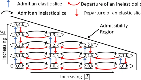
Fig. 2: Example of system model with the different states.

We define our space state S as follows. A states∈S is a

three-sized tuple (ni, ne, k |ni, ne∈ A)whereni andne are

the number of inelastic and elastic slices in the system at a

given decision time t, andk∈ {i, e, d} is the next event that

triggers a decision process. This can be either a new arrival of

a network slice request for inelastic and elastic slices (k=i

andk=e, respectively), or a departure of a network slice of

any kind that left the system (k=d). In the latter case,niand

ne represent the number of inelastic and elastic slices in the

system after the departure. Fig. 2 shows how the space state

S relates to the admissibility regionA.

The possible actions a ∈A are the following: A=G, D.

The actionGcorresponds to admitting the new request of an

elastic or inelastic slice; in this case, the resources associated with the request are granted to the tenant and the revenue

r=ρi,etis immediately earned by the infrastructure provider.

In contrast, actionDcorresponds to rejecting the new request;

in this case, there is no immediate reward but the resources remain free for future requests. Note that upon a departure

(k = d), the system is forced to a fictitious action D that

involves no revenue. Furthermore, we force that upon reaching a state in the boundary of the admissibility region computed in the previous section, the only available action is to reject

an incoming request (a=D) as otherwise we would not be

meeting the committed guarantees. Requests that are rejected are lost forever.

The transition rates between the states identified above are

derived next. Transitions to a new state withk=iandk=e

happen with a rateλiandλe, respectively. Additionally, states

with k = d are reached with a rate niµi+neµe depending

the number of slices already in the system. Thus, the average

time the system stays at states,T¯(s, a)is given by

¯

T(s, a) = 1

υ(ni, ne)

, (10)

whereni, andneare the number of inelastic and elastic slices

in state sandυ(ni, ne) =λi+λe+niµi+neµe.

We define a policy π(S), π(s) ∈ A, as a mapping from

each state s to an action A. Thus, the policy determines

whether, for a given number of elastic and inelastic slices in the system, we should admit a new request of an elastic or an inelastic slice upon each arrival. With the above analysis, given such a policy, we can compute the probability of staying at each of the possible states. Then, the long-term average

revenue R obtained by the infrastructure provider can be

computed as

R= ∑

ni,ne,k

P(ni, ne, k) (niρi+neρe), (11)

whereρiandρeare the price per time unit paid by an inelastic

and an elastic network slice, respectively.

The ultimate goal is to find the policyπ(S)that maximizes

the long term average revenue, given the admissibility region and the network slices requests arrival process. We next devise the Optimal Policy when the parameters of the arrival process

are knowna priori, which provides a benchmark for the best

possible performance. Later on, in Section 6, we design a learning algorithm that approximates the optimal policy.

5.2 Optimal policy

In order to derive the optimal policy, we build on Value Iteration [37], which is an iterative approach to find the optimal policy that maximizes the average revenue of an SMDP-based system. According to the model provided in the previous

section, our system has the transition probabilitiesP(s, a, s′)

detailed below.

Let us start with a =D, which corresponds to the action

where an incoming request is rejected. In this case, we have

that when there is an arrival, which happens with a rate λi

and λe for inelastic and elastic requests, respectively, the

request is rejected and the system remains in the same state. In case of a departure of an elastic or an inelastic slice, which

happens with a rate ofneµe orniµi, the number of slices in

the system is reduced by one unit (recall that no decision is

needed when slices leave the system). Formally, for a = D

ands= (ni, ne, i), we have:

P(s, a, s′) =

          

λi

υ(ni,ne), s′ = (ni, ne, i)

λe

υ(ni,ne), s′ = (ni, ne, e)

niµi υ(ni,ne), s

′ _{= (n}

i−1, ne, d) neµe

υ(ni,ne), s

′ _{= (ni, ne−1, d)}

. (12)

When the chosen action is to accept the request (a= G)

and the last arrival was an inelastic slice (k=i), the transition

probabilities are as follows. In case of an inelastic slice arrival,

which happens with a rate λi, the last arrival remains k=i,

and in case of an elastic arrival it becomesk=e. The number

of inelastic slices increases by one unit in all cases except of an

inelastic departure (rateniµi). In case of an elastic departure

(rate neµe), the number of elastic slices decreases by one.

Formally, fora=Gands= (ni, ne, i), we have:

P(s, a, s′) =

          

λi

υ(ni+1,ne), s

′_{= (ni+ 1, ne, i)}

λe

υ(ni+1,ne), s

′_{= (ni+ 1, ne, e)} (ni+1)µi

υ(ni+1,ne), s′= (ni, ne, d)

neµe

υ(ni+1,ne), s′= (ni+ 1, ne−1, d) . (13)

If the accepted slice is elastic (k=e), the system exhibits

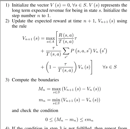
Algorithm 1 Value Iteration

1) Initialize the vectorV (s) = 0,∀s∈S.V(s)represents the long term expected revenue for being in states. Initialize the

step number nto 1.

2) Update the expected reward at timen+ 1, Vn+1(s) using

the rule

Vn+1(s) = max a∈A

[

R(s, a)

T(s, a)τ

+ τ

T(s, a)

∑

s′

P(s, a, s′)Vn (

s′)

+

(

1− τ

T(s, a)

)

Vn(s) ]

∀s∈S

3) Compute the boundaries

Mn= max

s∈S(Vn+1(s)−Vn(s)) mn= min

s∈S(Vn+1(s)−Vn(s))

and check the condition

0≤(Mn−mn)≤ϵmn

4) If the condition in step 3 is not fulfilled, then repeat from step 2

by one the number of elastic slices instead. Thus, for a=G,

s= (ni, ne, e), we have:

P(s, a, s′) =

          

λi

υ(ni,ne+1), s

′ _{= (ni, ne+ 1, i)}

λe

υ(ni,ne+1), s

′ _{= (ni, ne+ 1, e)}

niµi υ(ni,ne+1), s

′ _{= (ni−1, ne+ 1, d)} (ne+1)µe

υ(ni,ne+1), s′ = (ni, ne, d)

. (14)

A reward is obtained every time the system accepts a new slice, which leads to

R(s, a) =

    

0, a=D

tρi a=G, k=i

tρe a=G, k=e

. (15)

Applying the Value Iteration algorithm [37] for SMDP is not straightforward. The standard algorithm cannot be applied to a continuous time problem as it does not consider variable transition times between states. Therefore, in order to apply Value Iteration to our system, an additional step is needed: all the transition times need to be normalized to multiples

of a faster, arbitrary, fixed transition time τ [38]. The only

constraint that has to be satisfied byτ is that it has to be faster

than any other transition time in the system, which leads to

τ <minT(s, a), ∀s∈S,∀a∈A. (16)

With the above normalization, the continuous time SMDP corresponding to the analysis of the previous section becomes a discrete time Markov Process and a modified Value Iteration

algorithm may be used to devise the best policy π(S) (see

Algorithm 1). The discretized Markov Chain will hence

per-form one transition everyτ interval. Some of these transitions

correspond to transitions in continuous time system, while in the others the system keeps in the same state (we call the latter fictitious transitions).

!"#$%&'(&)*'+%$,&+*$,)

!"#$%&'(&$()*'+%$,&+*$,)

-).'/%0/)&12&'(&$()*'+%$,&+*$,)

-).'/%0/)&12&'(&)*'+%$,&+*$,)

!"#$++$3$*$%4& 5)6$1(

71*$,4&-)2$()"&5)6$1(

89:9;

8989; 89<9;

89=9; 89>9;

:989; =989; <989; :9:9; =9:9; <9:9;

=9=9; :9=9;

:9<9;

?(,/)'+$(6

?(

,/

)

'

+$

(

6

&

Fig. 3: Example of optimal policy for elastic and inelastic slices.

The normalization procedure affects the update rule of step 2 in Algorithm 1. All the transition probabilities P(s, a, s′) are scaled by a factor _T(s,aτ ′) to enforce that the system stays in the corresponding state during an average time

T(s, a′). Also, the revenue R(s, a) is scaled by a factor of

T(s, a)to take into account the fact that the rewardR(s, a)

corresponds to a period T(s, a) in the continuous system,

while we only remain in a state for aτduration in the discrete

system. In some cases, transitions in the sampled discrete time system may not correspond to any transition in the continuous time one: this is taken into account in the last term of the equation, i.e., in case of a fictitious transition, we keep in state Vn(s).

As proven in [30], Algorithm 1 is guaranteed to find the

optimal policy π(S). Such an optimal policy is illustrated in

Fig. 3 for the case where the price of inelastic slice is higher

than that of elastic slice (ρi > ρe). The figure shows those

states for which the corresponding action is to admit the new request (straight line), and those for which it is to reject it (dashed lines). It can be observed that while some of the states with a certain number of elastic slices fall into the admissibility region, the system is better off rejecting those requests and waiting for future (more rewarding) requests of inelastic slice. In contrast, inelastic slice requests are always admitted (within the admissibility region).

The analysis performed so far has been limited to network slice requests of size one. In order to extend the analysis to requests of an arbitrary size, we proceed as follows. We set the space state to account for the number of slices of each different class in the system (where each class corresponds to a traffic type and a given size). Similarly, we compute the

transition probabilitiesP(s, a, s′)corresponding to arrival and

departures of different classes. With this, we can simply apply the same procedure as above (over the extended space state) to obtain the optimal policy.

Following [39], it can be seen that (i) Algorithm 1 converges

to a certain policy, and (ii) the policy to which the algorithm

6

N3AC:

A DEEP LEARNING APPROACH The Value Iteration algorithm described in Section 5.2 pro-vides the optimal policy for revenue maximization under the framework described of Section 5.1. While this is very useful in order to obtain a benchmark for comparison, the algorithm itself has a very high computational cost, which makes it impractical for real scenarios. Indeed, as the algorithm has to

update all theV valuesV(s), s∈Sat each step, the running

time grows steeply with the size of the state space, and may become too high for large scenarios. Moreover, the algorithm is executed offline, and hence cannot be applied unless all

system parameters are known a priori. In this section, we

present an alternative approach, the Network-slicing Neural

Network Admission Control (N3AC) algorithm, which has a

low computational complexity and can be applied to practical scenarios.

6.1 Deep Reinforcement Learning

N3AC falls under category of the deep reinforcement learning (RL). With N3AC, an agent (the InP) interacts with the environment and takes decisions at a given state, which lead to a certain reward. These rewards are fed back into the agent, which “learns” from the environment and the past decisions

using a learning function F. This learning function serves to

estimate the expected reward (in our case, the revenue). RL algorithms rely on an underlying Markovian system such as the one described in Section 5. They provide the

following features: (i) high scalability, as they learn online on

an event basis while exploring the system and thus avoid a long

learning initial phase, (ii) the ability to adapt to the underlying

system without requiring any a priori knowledge, as they

learn by interacting with the system, and (iii) the flexibility

to accommodate different learning functionsF, which provide

the mapping from the input state to the expected reward when taking a specific action.

The main distinguishing factor between different kinds of

RL algorithms is the structure of the learning function F.

Techniques such as Q-Learning [40] employ a lookup table for

F, which limits their applicability due to the lack of scalability

to a large space state [41]. In particular, Q-Learning solutions

need to store and update the expected reward value (i.e., the

Q-value) for each state-action pair. As a result, learning the right action for every state becomes infeasible when the space state grows, since this requires experiencing many times the same state-action pair before having a reliable estimation of the Q-value. This leads to extremely long convergence times that are unsuitable for most practical applications. Additionally, storing and efficiently visiting the large number of states poses strong requirements on the memory and computational footprint of the algorithm as the state space grows. For the specific case studied in this paper, the number of states in our model increases exponentially with the number of network slicing classes. Hence, when the number of network slicing classes grows, the computational resources required rapidly become excessive.

A common technique to avoid the problems described above

for Q-learning is to generalize the experience learned from

some states by applying this knowledge to other similar states,

which involves introducing a different F function. The key

idea behind such generalization is to exploit the knowledge

obtained from a fraction of the space state to derive the right

action for other states with similarfeatures. There are different

generalization strategies that can be applied to RL algorithms. The most straightforward technique is the linear function approximation [42]. With this technique, each state is given as a linear combination of functions that are representative of the system features. These functions are then updated using standard regression techniques. While this approach is scalable and computationally efficient, the right selection of the feature functions is a very hard problem. In our scenario, the Q-values

associated to states with similar features (e.g., the number

of inelastic users) are increasingly non linear as the system becomes larger. As a result, linearization does not provide a good performance in our case.

Neural Networks (NNs) are a more powerful and flexible tool for generalization. NNs consist of simple, highly

inter-connected elements called neurons that learn the statistical

structure of the inputs if correctlytrained. With this tool, the

design of neuron internals and the interconnection between neurons are the most important design parameters. RL al-gorithms that employ NNs are called Deep RL alal-gorithms: N3AC belongs to this family. One of the key features of such a NN-based approach is that it only requires storing a very limited number of variables, corresponding to the weights and biases that compose the network architecture; yet, it is able

to accurately estimate theF function for a very large number

of state/action pairs. In the rest of this Section, we review the NNs design principles (Section 6.2) and explain how these principles are applied to a practical learning algorithm for our system (Section 6.3).

6.2 Neural networks framework

The fundamental building blocks of DRL algorithms are the following ones [43]:

• A set of labeled data (i.e., system inputs for which

the corresponding outputs are known) which is used to train the NN (i.e., teach the network to approximate the features of the system).

• A loss function that measures the neural network

perfor-mance in terms of training error (i.e., the error made when

approximating the known output with the given input).

• An optimization procedure that reduces the loss functions

!"#$

!"#$

!"#$

!"#$

!"#%$

!"#%$

!"#%$

!"#%$

!"#%%$

!"#%%$

!"

#

$

%&

!"#$%'()*+,

-$

%#

$

%&

w′ ij

w

′′ ij

./00+"'()*+,& -$%#$%'()*+,

wij

s₌

!

ij

w_ijx_i

12&3'4')5%/6)%/7"'1$"5%/7"

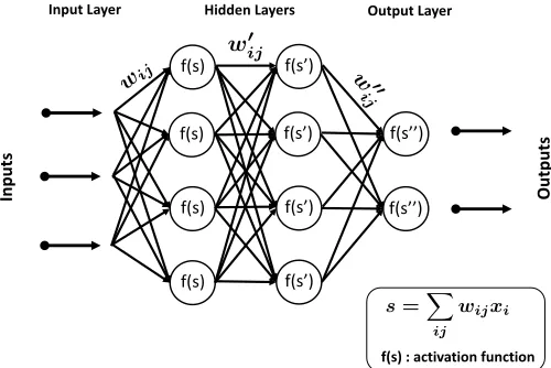
Fig. 4: Neural networks internals.

algorithm involves a number of design decisions to address the specificities of our problem, which are summarized in the following.

Neuron internal configuration. An exemplary NN is

illus-trated in Figure 4, where we have multiple layers of

inter-connected neurons organized as: (i) an input, (ii) an output

and (iii) one or more hidden layers. A neuron is a non-linear

element that executes a so-called activation function to the

linear combination of the weighted inputs. Many different activation functions are available in the literature spanning

from a linear function to more complex ones such as tanh,

sigmoid or the Rectified Linear Unit (ReLU) [44].N3AC employs the latter.

Neural Network Structure. One of the design choices that

needs to be taken when devising a NN approach is the the way neurons are interconnected among them. The most

common setup is feed-forward, where the neurons of a layer

are fully interconnected with the ones of the next. There

are also other configurations, such as the convolutional or

the recurrent (where the output is used as input in the next iteration). However, the best choice for a system like the one studied in this paper is the feed-forward. Indeed, convolutional networks are usually employed for image recognition, while recurrent are useful when the system input and the output have a certain degree of mutual relation. None of these match our system, which is memoryless as it is based on a Markovian approach. Furthermore, our NN design relies on a single hidden layer. Such a design choice is driven by the following

two observations: (i) it has been proven that is possible to

approximate any function using NN with a single hidden

layer [45], and (ii) while a larger number of hidden layers

may improve the accuracy of the NN, it also involves a higher complexity and longer training period; as a result, one should employ the required number of hidden layers but avoid building a larger network than strictly necessary.

Back-propagation algorithm selection. In classical ML

ap-plications, the NN is trained using a labeled dataset: the NN is fed with the inputs and the difference among the estimated output and the label is evaluated with the error function. Then, the error is processed to adjust the NN weights and thus reduce the error in the next iteration. N3AC adjusts

weights using a Gradient Descent approach: the measured error at the output layer is back-propagated to the input layer changing the weights values of each layer accordingly [44]. More specifically, N3AC employs the RMSprop [46] Gradient Descent algorithm.

Integration with the RL framework. One of the critical

requirements for N3AC is to operate without any previously known output, but rather interacting with the environment to learn its characteristics. Indeed, in N3AC we do not have any “ground truth” and thus we need to rely on estimations of the output, which will become more accurate as we keep exploring the system. While this problem has been extensively studied in the literature [43], [47], we need to devise a solution that is suitable for the specific problem addressed. In N3AC, we take as the output of the NN the average revenues expected at a given state when taking a specific decision. Once the decision is taken, the system transitions to the new state and we measure the average revenue resulting from the decision taken (0 in

case of a rejection andρtin case of an acceptance). Then, the

error between the estimated revenue and the measured one is used to train the NN, back-propagating this error into the weights. N3AC uses two different NNs: one to estimate the revenue for each state when the selected action is to accept the incoming request, and another one when we reject the request. Upon receiving a request, N3AC polls the two NNs and selects the action with the highest expected revenue; then, after the transition to the new state is performed, the selected NN is trained. More details about the N3AC operation are provided in the next section.

Exploration vs exploitation trade-off. N3AC drives the

selection of the best action to be taken at each time step. While choosing the action that maximizes the revenue at each step contributes to maximizing the overall revenue (referred

to asexploitationstep), in order to learn we also need to visit

new (still unknown) states even if this may eventually lead to

a suboptimal revenue (referred to as exploration step). This

procedure is especially important during the initial interaction of the system, where estimates are very inaccurate. In N3AC, the trade-off between exploitation and exploration is regulated

by theγ parameter, which indicates the probability of taking

an exploration step. In the setup used in this paper, we take

γ= 0.1. Once the NNs are fully trained, the system goes into

exploitation only, completely omitting the exploration part.

6.3 Algorithm description

In the following, we describe the proposed N3AC algorithm. This algorithm builds on the Neural Networks framework described above, exploiting RL to train the algorithm without a ground truth sequence. The algorithm consists of the following high level steps (see Algorithm 2 for the pseudocode):

• Step 1, acceptance decision:In order to decide whether to accept or reject an incoming request, we look at the expected average revenues resulting from accepting and rejecting a request in the two NNs, which we refer to

as the Q-values. Specifically, we define Q(s, a) as the

expected cumulative reward when starting from a certain

the optimal policy reward when starting from state 0, i.e.,

Q(s, a) =E

 lim

t_→∞ D_∑(t)

n=0

Rn−σt|s0=s, a0=a

  (17)

whereD(t)is the number of requests received in a period

t, Rn is the revenue obtained with the nth request and

σ = E[limt_→∞1_t

∑D(t)

n=0Rn|s0= 0] under the optimal

policy. Then, we take the decision that yields the highest Q-value. This procedure is used for elastic slices only, as inelastic slices shall always be accepted as long as there is sufficient room. When there is no room for an additional slice, requests are rejected automatically, regardless of their type.

• Step 2, evaluation: By taking a decision in Step 1, the

system experiences a transition from statesat stepn, to

states′at stepn+1. Once in stepn+1, the algorithm has

observed both the reward obtained during the transition

R(s, a) and a sample tn of the transition time. The

algorithm trains the weights of the corresponding NN

based on the error between the expected reward of s

estimated at stepn and the target value. This step relies

on two cornerstone procedures:

– Step 2a, back-propagation: This procedure drives the weights update by propagating the error measured back through all the NN layers, and updating the weights according to their gradient. The convergence time is driven by a learning rate parameter that is used in the weight updates.

– Step 2b, target creation: This procedure is needed to measure the accuracy of the NNs estimations during the learning phase. At each iteration our algorithm computes the observed revenue as follows:

ω=R(s, a, s′)−σtn+ max a′ Q(s

′_{, a}′_{), (18)}

whereR(s, a, s′)is the revenue obtained in the

transi-tion to the new state. As we do not have labeled data,

we useωto estimate the error, by taking the difference

between ω and the previous estimate Qn+1(s, a)and

using it to train the NN. When the NN eventually

converges, ω will be close to the Q-values estimates.

• Step 3, penalization:When a state in the boundary of the admissibility region is reached, the system is forced to reject the request. This should be avoided as it may force the system to reject potentially high rewarding slices. To

avoid such cases, N3AC introduces a penalty on the

Q-values every time the system reaches the border of the admissibility region. With this approach, if the system is brought to the boundary through a sequence of highly rewarding actions, the penalty will have small effect as the Q-values will remain high even after applying the penalty. Instead, if the system reaches the boundary following a chain of poorly rewarding actions, the impact on the involved Q-values will be much higher, making it unlikely that the same sequence of decisions is chosen in the future.

Algorithm 2 N3AC algorithm.

1) Initialize the Neural Network’s weights to random values. 2) An event is characterized by:s, a, s′, r, t(the starting state,

the action taken, the landing state, the obtained reward and the transition time).

3) Estimate Q(s′, a′) for each action a′ available in state s′ through the NN.

4) Build the target value with the new sample observation as follows:

target=R(s, a, s′)−σtn+ max a′ Q

(

s′, a′) (19)

wheretnis the transition time between two subsequent states

sands′after actiona.

5) Train the NNs through RMSprop algorithm:

5.1 Ifs ̸∈admissibility region boundary, train the NN with

the error given by the difference between the above target value (step 4) and the measured one.

5.2 Otherwise, train the NN corresponding to accepted

re-quests by applying a“penalty”and train the NN

corre-sponding to rejected requests as in step 5.1.

• Step 4, learning finalization: Once the learning phase is over, the NN training stops. At this point, at a given state we just take the the action that provides the highest expected reward.

We remark that the learning phase of our algorithm does not require specific training datasets. Instead, the algorithm learns from the real slice requests on the fly, during the real operation

of the system; this is the so-called exploration phase. The

training corresponding to such an exploration phase terminates when the algorithm has converged to a good learning status, and is triggered again when the system detects changes in the system that require new training.

7

P

ERFORMANCE

E

VALUATION

In this section we evaluate the performance of N3AC via simulation. Unless otherwise stated, we consider a scenario with four slice classes, two for elastic traffic and two for inelastic. Service times follow an exponential distribution with

µ = 5 for all network slices classes, and arrivals follow a

Poisson process with average rates equal to λi = 2µ and

λe = 10λi for the elastic and inelastic classes, respectively.

We consider two network slice sizes, equal toC/10andC/20,

where C is the total network capacity. Similarly, we set the

throughput required guarantees for elastic and inelastic traffic

to Ri = Re = Cb/10. Two key parameters that will be

employed throughout the performance evaluation are ρe and

ρi, the average revenue per time unit generated by elastic

and inelastic slices, respectively (in particular, performance depends on the ratio between them). The rest of the network setup (including the users’ mobility model) is based on the scenario described in Section 4.2.

Following the N3AC algorithm proposed in the previous section, we employ two feed-forward NNs, one for accepted requests and another one for rejected. Each neuron applies a ReLU activation function, and we train them during the exploration phase using the NNs RMSprop algorithm

imple-mentation available in Keras (https://keras.io/); the learning

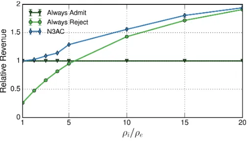
Fig. 5: Revenue vs.ρi/ρe.

equal to 0.001. The number of input nodes in the NN is equal

to the size of the space state (i.e., the number of considered

classes plus one for the next requestk), the number of neurons

in the hidden layer equal to 40 for the scenario described in Sections 7.3 and 7.4 and 20 for the others, and the output layer is composed of one neuron, applying a linear function. Note that, while we are dealing with a specific NN structure, one of the key highlights of our results is that the adopted structure works well for a wide range of different 5G networks.

In the results given in this section, when relevant we provide the 99% confidence intervals over an average of 100 experiments (note that in many cases the confidence intervals are so small that they cannot be appreciated).

7.1 Algorithm Optimality

We first evaluate the performance of the N3AC algorithm (which includes a hidden layer of 20 neurons) by comparing it

against: (i) the benchmark provided by the optimal algorithm,

(ii) the Q-learning algorithm proposed in [30], and (iii) two

naive policies that always admit elastic traffic requests and always reject them, respectively. In order to evaluate the optimal algorithm and the Q-learning one, which suffers from scalability limitations, we consider a relatively small scenario. Figure 5 shows the relative average reward obtained by each of these policies, taking as baseline the policy that always admit all network slice requests (which is the most straightforward algorithm).

We observe that N3AC performs very closely to the Q-learning and optimal policies, which validates the proposed algorithm in terms of optimality. We further observe that the revenue improvements over the naive policies is very

substan-tial, up to 100% in some cases. As expected, for small ρi/ρe

the policy that always admits all requests is optimal: in this case both elastic and inelastic slices provide the same revenue.

In contrast, for very largeρi/ρeratios the performance of the

“always reject” policy improves, as in this case the revenue obtained from elastic traffic is (comparatively) much smaller.

7.2 Learning time and adaptability

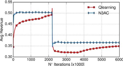
One of the key advantages of the N3AC algorithm as compared with Q-learning is that it requires a much shorter learning time. This is due to the fact that with N3AC the knowledge acquired

Fig. 6: Learning time for N3AC and Q-learning.

Fig. 7: Performance under changing conditions.

at each step is used to update the Q-values of all states, while Q-learning just updates the Q-value of the lookup table for the state being visited. To evaluate the gain provided by the NNs in terms of convergence time, we analyze the evolution of the expected revenue over time for the N3AC and the Q-learning algorithms. The results are shown in Figure 6 as a function of the number of iterations. We observe that after few hundred iterations, N3AC has already learned the correct policy and the revenue stabilizes. In contrast, Q-learning needs several thousands of iterations to converge. We conclude that N3AC can be applied to much more dynamic scenarios as it can adapt to changing environments. Instead, Q-learning just works for relatively static scenarios, which limits its practical applicability. Furthermore, Q-learning cannot scale to large scenarios, as the learning time (and memory requirements) would grow unacceptably for such scenarios.