Article
1
A Novel High Accuracy PV Cell Model Including
2Selfheating and Parameter Variation
3Aurel Gontean1,*, Septimiu Lica1, Szilard Bularka1, Roland Szabo1 and Dan Lascu1 4
1 Politehnica University Timisoara, Romania; [email protected] 5
* Correspondence: [email protected]; Tel.: +40-745-121-383 6
Abstract: This paper proposes a novel model for a PV cell with parameters variance dependency on 7
temperature and irradiance included. The model relies on commercial available data, calculates the 8
cell parameters for standard conditions and then extrapolates them for the whole operating range. 9
An up-to-date review of the PV modeling is also included with series and parallel parasitic 10
resistance values and dependencies discussed. The parameters variance is analyzed and included 11
in the proposed PV model, where the self-heating phenomenon is also considered. Each parameter 12
variance is compared to the results from different authors. The model includes only standard 13
components and can be run on any SPICE-based simulator. Unlike other approaches that consider 14
the internal temperature as a parameter, our proposal relies on air temperature as an input and 15
computes the actual internal temperature accordingly. Finally, the model is validated via 16
experiments and comparisons to similar approaches are provided. 17
Keywords: PV cell; model; simulation; SPICE; selfheating; parameters variation 18
19
1. Introduction 20
PV cells have been extensively studied in the last decades [1-8] as solar energy is more and more 21
accepted as a viable alternative to traditional energy sources. Modeling the PV behavior is useful for 22
system design, planning, research and training. The goal of this work is to develop an accurate model 23
for a PV Cell, expandable to a whole module, using affordable tools and taking into account 24
parameters variations. LTSpice [9] was chosen as the simulation tool due to its free cost and wide 25
acceptance, Visual Studio Express [10], also a free tool, was used for parameters estimation and 26
solution validation. Finally, S-Math Studio [11] was selected for the trial and error different 27
evaluations. The solution implies a reasonable computing power and provides fast convergence. The 28
model itself is portable, as it uses only standard components and is also vendor independent. The 29
input data is usually provided from the manufacturer’s datasheet or can be obtained via experiments. 30
Unlike other approaches, the model input temperature is the ambient/air temperature, and 31
based on actual irradiance the model calculates the internal (silicon) temperature and provides the 32
actual I-V and P-V curves. 33
The paper is organized as follows: Section 2 briefly analyzes the classical PV model and its 34
equations. Section 3 deals with the information provided by the PV cell datasheet and the equipment 35
involved in measurements. Finding the solution for the PV cell model is analyzed in section 4, with 36
section 4.1 introducing the solving algorithm. A review of parameters variation is the subject for 37
Section 4.2, including the real operating conditions, when the PV solar cell is selfheating. The new PV 38
cell model is proposed in Section 4.3, the experimental results are exposed in Section 5, while 39
conclusions are presented in Section 6. 40
41 42 43 44 45
2. The Classical PV Cell Model 46
The equivalent circuit of a solar cell is investigated in several prior works [12 – 38]. It is generally 47
accepted that a PV cell can be modeled by the circuit in Figure 1, including one [12 - 32], two [33 – 35] 48
and rarely three or more diodes [36 - 37]. 49
50
Figure 1. Equivalent circuit of a photovoltaic cell. 51
52
In Figure 1, current source models the photo generated current, with a linear dependency 53
on the irradiance. The first diode, , is associated with the diffusion mechanism. The second diode, 54
, is inserted to include the effect of charge recombination. Resistance represents the cell series 55
resistance and resistance the cell parallel (shunt) resistance. Resistance is related to losses in 56
cell solder bonds, wires, junctions and so on and it is usually bellow 1Ω. Resistance is related to 57
the leakage current through the high conductivity shunts across the p-n junction and is usually in the 58
order of ten of ohms to several kΩ. The circuit in Figure 1 can be extended to any combination of 59
series – parallel cells within a PV module (array). In this paper we shall consider only one diode 60
in the model, , neglecting . The equations will be provided in a general form, while the 61
simulations and experiments will be conducted for a single cell, that is for = = 1. 62
Referring to Figure 1, according to Kirchhoff’s current law (KCL), one can write: 63
= − exp + − 1 − + (1)
64
where is the diode reverse saturation current, is the electron charge, is the Boltzmann 65
constant, is the actual silicon temperature and is the ideality factor of the diode. 66
Current linearly depends on irradiation and temperature [15], [18]: 67
= , + ∆ (2)
At the maximum power point, using (1), the maximum power can be derived [22]: 68
= = − + − 1 − + (3)
Even in (1) and (3) is considered equal to , a more accurate formula for is [22]: 69
, = + , (4)
A good overview of the PV cell performance can be found in [12], where an empirical formula 70
for the fill factor is introduced, considering the single diode model: 71
= −ln 0.72 +
3. Materials, Methods and Equipment 72
For our experiments we have chosen a high efficiency low cost monocrystalline Silicon PV solar 73
cell, unmounted in panels [39]. The datasheet of the PV cell offers a limited amount of data, 74
summarized in Table 1. 75
76
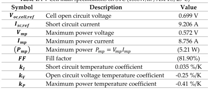
Table 1. PV Cell main specifications on STC (1000W/m2, AM 1.5, 25°C) 77
Symbol Description Value
, , Cell open circuit voltage 0.699 V
, Short circuit current 9.206 A
Maximum power voltage 0.572 V
Maximum power current 8.756 A
Maximum power = (5.21 W)
Fill factor (81.90%)
Short circuit temperature coefficient 0.035 %/K Open circuit voltage temperature coefficient -0.25 %/K Maximum power temperature coefficient -0.41 %/K 78
It is important to note that = 0.75 … 0.9 ∙ for any solar cell. This is a good starting point 79
for any simulation or MPPT algorithm implementation. 80
The data from the datasheet is confusing, as: 81
1. The claimed maximum power (5.21W) differs from = 5.01W. This latter value will be 82
considered subsequently. 83
2. The claimed fill factor (81.90%) differs from the standard definition = ∙
, ∙ , = 77.82%
84
The empirical equation (5) yields an approximate result ( ≅ 84.08%) when compared to the 85
datasheet values (Table 1). 86
The irradiance was measured with a Klipp and Zonen SHP1 pyrheliometer with integrated 87
temperature sensor for temperature compensation. The internal silicon temperature was determined 88
with a FLIR E8 infrared camera and a PT1000 temperature sensor on the rear of the PV cell. In order 89
to obtain reliable data, the PT1000 temperature sensor was glued with high thermally conductive 90
adhesive to the backside metal coating of the PV cell. The ambient temperature was measured using 91
the National Instruments NI USB T01 interface. Due to the extremely low internal series resistance 92
, several series cells were carefully wired and a Kelvin connection had to be used for voltage 93
measurements. The measurements were performed under real life conditions, when the solar 94
irradiance was maximum with the PV cells oriented toward the sun on 45 degree inclined support. 95
The load was an ET Instrument ESL-Solar, configured in MPPT mode. 96
97
4. Classical Model Solving 98
Several ways for solving the equations have been proposed [17, 20, 22, 26, 27, 28, 30, 32]. One of 99
the difficulties is the implicit nature of equation (1) regarding . This has been addressed by various 100
techniques, ranging from pure mathematical approaches (including Lambertian W-Function, [31]) to 101
pure numerical solutions, mainly in MATLAB [5, 6, 16, 35]. Later models [40 - 52] take into account 102
the parameters variation with temperature and irradiance. However the most common approach 103
considers the internal PV temperature as an independent parameter and plots the I-V family curves 104
for different temperatures. This aspect will be covered in the subsequent sections. It has to be stressed 105
out that the exponential nature of equation (1) determines that a small variation in any of the terms 106
involved in the exponential term to substantially modify the final result. This aspect will be addressed 107
4.1. Solving the Equations for the Classical PV Model
109
The method introduced here is an extension of the method proposed by Villalva et al. [22] and 110
involves the following steps: 111
1. Compute 112
2. For validation purposes determine the limits , and ,
113
3. For all values between 0, , with , as increment, numerically solve (1) for the MPP.
114
4. When the maximum power error is below the imposed threshold error, is established and 115
can be computed. 116
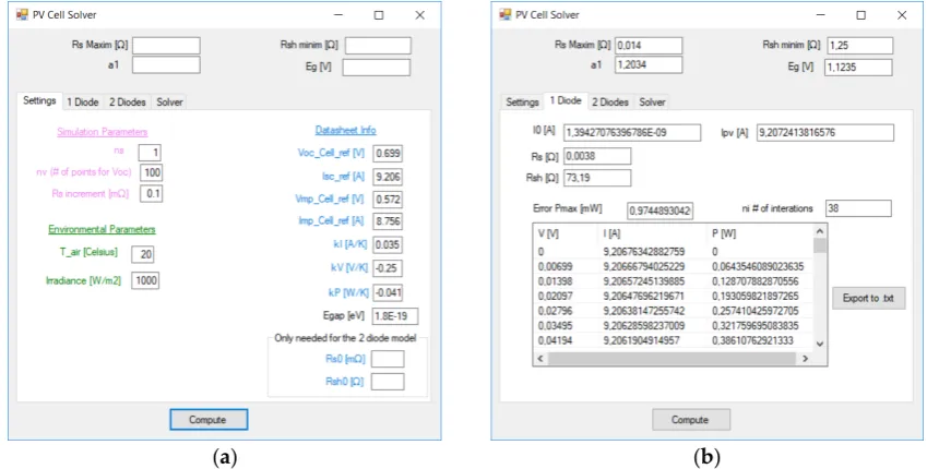
A VB.net application has been developed by the authors in order to numerically solve and 117
compute the model parameters. The application can be downloaded from http://tess.upt.ro. Figure 2 118
depicts a print screen for the initial parameter passing (a) and the results (b). 119
(a) (b)
Figure 2. VB.net PV Cell solver: (a) Entering parameters values; (b) Getting the solution. 120
In our case, using the values taken from the datasheet for = = 1, it results that: 121
, =
−
= 14 Ω (6)
122
, =
, − − , = 1.25 Ω (7)
These limits are important to set reliable ranges for the algorithm. The final results are listed in 123
Table 2. 124
Table 2. Vb.net application results 125
Symbol Description Results
, Photo generated current 9.207 A
, Reverse diode current 1.39427 nA
, Maximum Rs value (initial guess) 14 mΩ
, Series resistance 3.8 mΩ
, Minimum Rsh value (initial guess) 1.25 Ω
, Parallel resistance 73.19 Ω
, Ideality factor 1.2034
, Bandgap energy 1.795E-19 eV
Several attempts have been made for finding explicit expressions for and based on 126
actual datasheet data. For example, Cubas et al. [31] offer the formula (with as an argument, 127
considering = 1): 128
= − − − −
− − − (8)
For the above data, the formula (8) yields a result of 59.43 Ω, compared to the actual value 129
of 73.19 Ω. 130
In a simplified model ( → ∞), Xiao et al. [18] propose for the following relationship (again 131
= 1): 132
=
1 − + −
(9)
Here (9) yields = 0.7 Ω, quite far from its actual value (3.8 mΩ). 133
4.2. Parameters variation for different conditions
134
The parameters in equations (1) – (4) are not constant over the environmental conditions, as 135
, , , , depend on temperature and irradiance. A brief review of these dependencies is 136
provided bellow. 137
4.2.1. Diode saturation current – 138
Phang et al. [13] show that if is below 10A, can be derived as in (10): 139
= − − (10)
140
in (10) yields a very good result of 1.3969 nA vs 1.39427nA obtained in Table 2. 141
Gow and Manning [15] were among the first to claim that: 142
= (11)
The temperature dependence of this current is more detailed expressed by [16], [20]: 143
= ,
1
−1 (12)
144
where is the bandgap voltage of the semiconductor ( = 1.1 … 1.3 for Si at 25 °C). 145
, can be derived from (1) at the reference temperature as:
146
, = ,
exp , − 1 (13)
147
According to Vilalva et al. [22], , can be further improved:
148
, = ,
+ ∆
exp , + ∆ − 1 (14)
In subchapter 4.6.3 of [8], van Zeghbroeck states an equation in which , can be derived
150
from, that can offer an alternate way to estimate , :
151
=
1 +
,
1 + (15)
This proves to be not very accurate in our case, as with the values from Table 1, , from (15)
152
results 0.085 nA, quite far from the actual value (1.39427 nA). 153
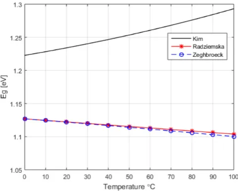
4.2.2. Band gap energy and bandgap voltage – , 154
Van Zeghbroeck [8] shows that the bandgap energy, , exhibits a small temperature 155
dependence as in (16). 156
= 1.166 −0.000477 ∙
636 + (16)
From (16), , = 1.121 eV for silicon cells at 25°C. This is the value considered in Table 1.
157
In contrast, Kim et al. [23] define the variance for for silicon to be: 158
= 1.16 −7.02 ∙ 10 ∙
− 1108 (17)
Both (16) and (17) fit in the [1.1 … 1.3V] interval specified when equation (12) was introduced. 159
In our approach shown in Figure 3, we adopted the Van Zeghbroeck proposal because it will finally 160
lead to a more realistic value for and close to the linear approximation of against temperature 161
suggested by Radziemska and Klugmann [40], which indicate a temperature coefficient d ⁄d = 162
−2.3 ∙ 10 eV K⁄ . 163
164
165
Figure 3. variation against temperature according to several authors 166
4.2.3. Series resistance – 167
Honsberg and Bowden [7] show that does not influence , but close to the open-circuit 168
voltage, the I-V curve is affected by . An initial estimation for is to find the slope of the I-V 169
curve at the open-circuit voltage point (18): 170
= −d
171
In our case, = 11 mΩ (while = 3.8mΩ, as it will later be shown). 172
Cuce and Bali [43], Cuce et al. [47] and Singh et al. [42] claim that linearly decreases with the 173
temperature. Obviously, reducing yields an increase in the output current. 174
A PV Cell model is also available in MATLAB Simscape [52]. It consists of the same circuit as in 175
Figure 1, where the user can choose between: 176
• An 8-parameter model, where equation (1) describes the output current
177
• A 5-parameter model that neglects in Figure 1 and the value of the shunt resistor is infinite.
178
Both models adjust the resistance values and current parameters as a function of temperature. 179
Resistance is assumed to be given by (19): 180
= , (19)
where is the temperature exponent for . is 0 by default and when modified has to be 181
positive. 182
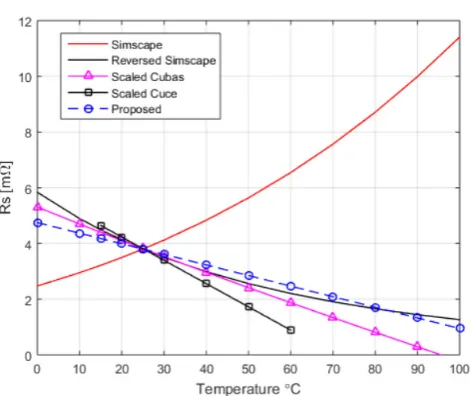
Figure 4 summarizes all these above dependencies. In order to have the results in the same range, 183
Cubas et al. [31] and Cuce et al. [47] results were scaled, and equation (19) was re-written as in (20), 184
interchanging with and was estimated as 4.9 for the best fit. A linear dependency is easy 185
to implement, but might also lead to results not physically true (for example Cuce et al. [47] data lead 186
to negative resistances for temperatures over 75°C and so does Cubas et al. [31] over 97°C). 187
= , (20)
where | | = | |. 188
189
190
Figure 4. variation against temperature by several authors 191
The linear law (21) was adopted for and we chose = −0.01K , again for the best fit. 192
= , 1 + − (21)
193
4.2.4. Parallel resistance – 195
Honsberg and Bowden [7] and Jung and Ahmed [25] showed that the shunt resistance of a solar 196
cell can be determined from the slope of the I-V curve close to the short-circuit point, yielding a fair 197
approximation for : 198
= −d
d (22)
199
From Figure 11.a, = 73.18 Ω, very close to the accurate solution = 73.19 Ω, as it will 200
later be illustrated. 201
Cuce and Bali [43] and Cuce et al. [47] claim that the shunt resistance linearly decreases with 202
temperature. They explain this decrease in terms of a combination of tunneling and trapping– 203
detrapping of the carriers through the defect states in the space-charge region of the device. These 204
defect states act either as recombination centers or as traps depending upon the relative capture cross 205
sections of the electrons and holes for the defect. Temperature dependency for is however more 206
complicate. 207
is again modeled in MATLAB Simscape like (23): 208
= , (23)
where is the temperature exponent for . is 0 by default and when modified has to be 209
positive. 210
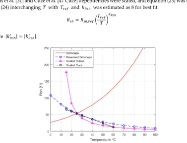
Figure 5 summarizes all these equations. In order to bring the results in the same range, 211
Cubas et al. [31] and Cuce et al. [47 Cuce] dependencies were scaled, and equation (23) was re-written 212
as in (24) interchanging with and was estimated as 8 for best fit. 213
= , (24)
where | | = | |. 214
215
Figure 5. variation over temperature by several authors 216
Although influence is small in the overall model, for an accurate modeling and especially 217
for larger temperature ranges linear variation is not realistic. Therefore in our model described 218
4.2.5. Ideality diode factor – 220
Some authors consider the ideality factor as being constant over the operating temperature range 221
and with a generic value for in the interval [1, 1.5] for every kind of cell [22], [31]. Cuce et al. [29] 222
propose = 1.2 for monocrystalline silicon cells, and = 1.3 for polycrystalline ones. Some 223
studies indicate a linear decreasing with temperature [18]. Cubas et al. [31] say that “the lack of 224
accuracy produced when considering the ideality factor as constant is generally reduced, given that 225
variations of this parameter only affects the curvature of the I-V curve.” This is arguable, as 226
interferes in an exponential dependency and small variations of lead to significant changes in 227
,and finally in . One might say that picking a random in the above specified range will be
228
balanced by a different , so only the pair , matters. However this approach is misleading, as 229
it may induce impossible physical solutions. 230
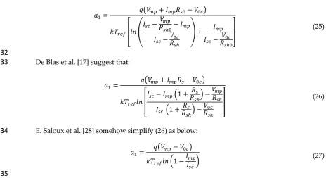
Phang et al. [13] have the following proposal: 231
= + −
− −
− + −
(25)
232
De Blas et al. [17] suggest that: 233
= + −
− 1 + −
1 + −
(26)
E. Saloux et al. [28] somehow simplify (26) as below: 234
235
In the algorithm of Villalva [53], a different formula is introduced. Considering that for 236
crystalline silicon = 1.8J, becomes 1.1235V and the following formula provides a good result1,
237
thus eliminating a trial and error time consuming for the initial guess of : 238
=
−
− 3 − (28)
The results for are summarized in Table 3, with a very good correlation between (25), (26) 239
and (28). This is the reason we have adopted the Villalva value of 1.2034. 240
Table 3. Different values 241
accepted range
Phang, equation (25)
De Blas, equation (26)
Saloux, equation (27)
Villalva, equation (28)
1 – 1.5 1.1952 1.2016 1.6377 1.2034
242
1 Formula (28) was adapted from [53], as the additional presence of the in the initial formula
provided correct results only for = 1
= −
Xiao et al. [18] specify a linear decreases of the ideality factor with the temperature for the Shell 243
ST40 module, ranging from 1.85 to 1.15, corresponding to 5 to 45 Celsius degree variance respectively. 244
From the data plotted in their work, the following law can be adopted: 245
= 7.013 − 0.01875 ∙ (29)
Such approach must be taken with extreme care, as it is a common practice to operate often at 246
temperatures higher than 48°C, where (29) yields = 1 (or 0 at 100°C) 247
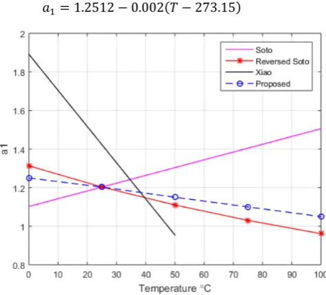
De Soto at al. [20] come with a different proposal: 248
= , (30)
which has a wrong slope. For a proper variation and should be reversed as follows: 249
= , (31)
250
Our experiments presented in Figure 6 yielded a different result, closer to reversed Soto (31), 251
according to the following linear dependency: 252
= 1.2512 − 0.002 − 273.15 (32)
253
Figure 6. vs temperature 254
4.2.6. Selfheating Phenomenon 255
It is a common practice to express the internal cell temperature, based on Normal 256
Operating Cell Temperature (NOCT) data, when the module is mounted 45° from horizontal. 257
= + − 20
800 (33)
Here = 800W m , = 20°C and airflow is 1 ⁄ [45]. 258
The internal temperature of the PV was of permanent concern for the researchers [40 - 42], [46], 259
but in most situations just an uncorrelated dependency is studied. Simply the temperature 260
dependency of the I-V characteristic without acknowledging neither the real, actual temperature of 261
the PV nor parameter variation is considered. Advanced simulators software packages include such 262
features, MATLAB Simscape [52] being one of them. 263
In a recent work, Krac and Górecki [55] introduced a thermal model for the PV cell, where the 264
capacitor, a voltage source related to the ambient temperature and a current source that represents 266
the total dissipated power within the PV. They claim that “for the maximum allowable value of the 267
panel forward current (equal to 8 A), a self-heating phenomenon causes an increase in the panel 268
temperature value equal only by 12°C.” In our experiments, we acquired a rather extended influence, 269
ranging from 20 to 30 °C. 270
Opposite to [54] and [55], the power dissipated by the PV cell is taken into account from the 271
dissipative elements, which are resistive in our model. The energy flows from the two current sources 272
to the resistors and the external circuit. Two or three current sources (or even diodes) are used in 273
order to model different phenomena that take place inside the PV cell, the photoelectric effect and 274
the behavior of p-n junction [8]. 275
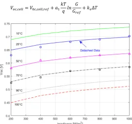
4.2.7. Open circuit voltage - 276
Ishaque and Salam [27] propose for the , the following variation (34), which proves good
277
correlation with the datasheet info and experimental data – see also Figure 7: 278
, = , , + + ∆ (34)
279
Figure 7. , vs Irradiance for different temperatures. Solid and dashed lines are given by (33), while
280
symbols correspond to experimental data. 281
Even (34) is not necessary for the model, it is another starting point for computing . 282
4.3. The New Proposed PV Cell Model
283
The proposed model is presented in Figure 8. The upper section consists of standard elements, 284
while the thermal modeling is ensured by the lower section. Here the current source labeled 285
simulates the power dissipated in the cell, the voltage labeled is the cell temperature and the air 286
temperature is modeled by the voltage source . The thermal resistance models the thermal 287
flow through the system structure, in our case the PV cell. The thermal capacitance models the 288
thermal inertia of the PV cell. Both and emulate all thermal transmission phenomena 289
(conduction, convection and radiation) and depend of the materials, the finishing of the surfaces and 290
292
Figure 8. The new proposed electrical and thermal model of the PV cell. 293
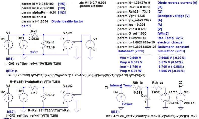
The practical LTSpice model implementation is depicted in Figure 9. The upper circuit addresses 294
the standard conditions (for reference and validation), while the middle section deals with the 295
thermal model of the PV solar cell. The power associated with the circuit also includes the power due 296
to the irradiance scaled with the cell area and the electrical power dissipated in and . 297
298
Figure 9. LTSpice PV Cell proposed model. 299
The thermal parameters and were extracted from experimental data. After a set of data 300
was acquired, the temperature against time curve variation was fit and the time constant and the 301
steady state value were determined. Unlike Górecki and Krac [54 - 56], we considered no dissipated 302
power occurs in the BD2 current source of the model in Figure 9, as it makes no physical sense. 303
5. Experimental Results 306
Figure 10 exhibits the simulated and the measured internal temperature of the PV cell and the 307
dissipated power variation. It is worth mentioning that the corresponding NOCT for the temperature 308
in Figure 9 is 47.2°C. 309
310
Figure 10. PV Cell dissipated power and temperature variation against voltage at STC. 311
Table 4 summarizes the main results for both the proposed model and the experiments 312
performed for the PV cell. It can be observed that perfect agreement between the simulated and 313
measured results is achieved. 314
315
Table 4. Comparison of the results at STC (25 Celsius, 1000 W/m2) 316
Symbol Description Datasheet
Value
Proposed Model
Model Error vs Datasheet
[%]
Experimental Values Results Error vs
Datasheet [%]
, , Cell open circuit voltage 0.699 V 0.6985 V -0.07% 0.693 V -0.86
, Short circuit current 9.206 A 9.206A 0% 9.221 A 0.16 Maximum power voltage 0.572 V 0.575 V 0.52% 0.569 V -0.52 Maximum power current 8.756 A 8.705 A -0.58% 8.731 A -0.29 Maximum power
= 5.01 W 5.005 W -0.06% 4.968 W -0.81
Fill factor 77.83% 77.84% 0.01% 77.52% -0.40 317
The final validation of the model is presented in Figure 11 and Figure 12. Here the I-V and P-V 318
characteristics of the PV cell are plotted at the reference temperature and at the operating 319
temperature. Experimental data is represented with markers while the lines correspond to simulated 320
results with the model proposed. A good correlation between the model and the experiments can be 321
noticed. 322
Figure 12 (a) displays the serial resistance influence on the output current and power. The 323
solid lines graphs correspond to a fixed while the dashed lines correspond to variable with 324
all the parameters included. At MPP a 98 mW power increase was observed. As estimated before, 325
has a minor influence on the PV output – only 4.6 mW power decrease at MPP could be noticed, 326
as displayed in Figure 12 (b). It is worth mentioning that in all cases the model self-computes the 327
(a) (b)
Figure 11. I-V and P-V curves – simulation and experiments. (a) I-V curves at 25°C (upper lines) and with all 329
parameters variation included (lower lines) – internal temperature is 54°C. (b) P-V curves at 25°C (upper lines) 330
and with all parameters variation included (lower lines) – internal temperature is 54°C. 331
332
(a) (b)
Figure 12. and influence and the performance. (a) increase with temperature (25°C to 54°C) 333
determines an increase in the output current and power (b) has no significant influence on the performance. 334
PV arrays compared (Table 5) were monocrystalline (Shell SP-70, MSMD290AS-36.EU and 335
multycrystaline (Kyocera KG200GT, MSP300AS-36.EU, MSP290AS-36.EU, Sharp ND-224uC1) 336
337
Table 5. Datasheet available information for several commercial PV arrays 338
PV Type [ ] [ ] [ ] [ ] [ ⁄ ] [ ⁄ ]
Shell SP-70 36 21.4 16.5 4.24 4.7 -76 2
MSMD290AS-36.EU 72 44.68 37.66 7.7 8.24 -138.508 3.296
MSP290AS-36.EU 72 44.32 37.08 7.82 8.37 -146.256 3.348
KG200GT 54 32.9 26.3 7.61 8.21 -123 3.18
Sharp ND-224uC1 60 36.6 29.3 7.66 8.33 -131.76 4.4149
339
All the data from Table 5 was processed with the above proposed algorithm and the results are 340
listed in Table 6, along with similar results from other researchers. 341
Table 6. Comparison between previous solutions and our proposed model 345
PV Type Solution [ ] [ ] [ ] [ ]
Shell SP-70 Ishaque* [35] 1&2.2 510 91 4.7 0.421;0.421
Proposed 1.022 505 73.85 4.732 0.657
MSMD290AS-36.EU Cubas [31] 1.1 130 316 8.24 2.36
Proposed 1.0 159 194 8.247 0.243
MSP290AS-36.EU Cubas [31] 1.1 162 331 8.37 2.86
Proposed 1.02 191 230 8.377 0.513
KG200GT
Ishaque* [35] 1&2.2 320 160.5 8.21 0.422;0.422 Sumathi et al. [5] 1.3 221 415.4 8.214 98.25
Proposed 1.08 305 186 8.223 2.15
Sharp ND-224uC1 Proposed 1.06 316 108 8.354 1.41
* Ishaque at al. [35] use a 2 diode model with equal saturation currents 346
347
The final validation of the model was by applying the introduced model and computation 348
method for the MSMD290AS-36.EU monocrystalline PV cell array and compare the results to the 349
ones provided by Cubas et al. [31], as shown in Figure 13. As it can be seen, a good correlation exists 350
between the two approaches. 351
(a) (b)
(c) (d)
Figure 13. Final model validation by comparison for the MSMD290AS-36.EU monocrystalline PV cells. (a) I-V 352
curves at 25°C; (b) P-V curves at 25°C (c) I-V curves at 54°C (d) P-V curves at 54°C. 353
6. Conclusions 355
A new thermo-electrical model for the PV cell was introduced. The model proved to be accurate, 356
while considering parameter variation and selfheating phenomenon. Only free available tools were 357
used during modeling. The literature analysis proved discrepancies between authors when studying 358
parameter variation and proposals have been submitted. 359
As other authors have mentioned, influence is relatively reduced in the model. However 360
proved to be a major factor. displayed a small variance with temperature. Resistance 361
influence is important but sometimes shadowed by the wiring. The proposed model was accurately 362
confirmed and validated by the experiments. 363
364
Acknowledgments: This work was supported by a grant of the Romanian National Authority for Scientific 365
Research and Innovation, CNCS/CCCDI - UEFISCDI, project number PN-III-P2-2.1-PED-2016-0074, within 366
PNCDI III. 367
Author Contributions: All of the authors have contributed to this research. Aurel Gontean conceived and 368
designed the study. Aurel Gontean and Septimiu Lica carried out the simulation. Szilard Bularka performed the 369
experiments. Dan Lascu analyzed the data. Aurel Gontean wrote the paper. Dan Lascu reviewed the manuscript. 370
All authors read and approved the manuscript. 371
Conflicts of Interest: The authors declare no conflict of interest. 372
Nomenclature 373
Main Symbols
374
Diodeideality factor 375
, Diodeideality factor at 25°C
376
Thermal capacitance of the cell, a lumped parameter 377
Bandgap energy 378
Fill factor 379
Actual irradiance on cell surface 380
Reference irradiance, 1000 W/m2 381
Solar cell current 382
Saturation current of the modeled diode, due to diffusion 383
, Saturation current of the modeled diode, due to diffusion, at 25°C
384
Current at maximum power point 385
Photo generated current 386
, Photo generated reference current at 25°C
387
Short circuit current of the solar cell 388
, Short circuit current of the solar cell at 25°C
389
Boltzmann constant 390
Current temperature coefficient, A/K 391
Voltage temperature coefficient, V/K 392
Power temperature coefficient, W/K 393
, , temperature exponent 394
, , temperature exponent in Matlab 395
Number of series cells 396
Number of parallel cells 397
= Maximum power 398
Electron charge 399
Cell series resistance 400
, Cell series resistance at 25°C
401
Cell series resistance based on slope close to 402
Cell parallel (shunt) resistance 403
, cell parallel (shunt) resistance, at 25°C
cell parallel (shunt) resistance based on slope close to 405
Thermal resistance of the cell, a lumped parameter 406
solar cell temperature, [K] 407
= reference temperature 298 K 408
∆ = − temperature difference
409
ambient/air temperature, [°C] 410
internal PV cell temperature, [°C] 411
solar cell voltage 412
solar array open circuit voltage 413
, solar array open circuit reference voltage at 25°C
414
, solar cell open circuit voltage
415
, , solar cell open circuit reference voltage at 25°C
416
voltage at maximum power point 417
bandgap voltage 418
= / diode thermal voltage 419
Abbreviations
420
AM Air Mass
421
KCL Kirchhoff’s current law 422
MPP Maximum power point 423
MPPT Maximum Power Point Tracking 424
NOCT Normal Operating Cell Temperature 425
PV Photovoltaic 426
STC Standard Test Conditions (cell temp. 25°C; irradiance 1000 W/m2; air mass 1.5) 427
Greek Symbols
428
series resistance temperature coefficient (linear law) 429
430
References 431
1. Rauschenbach, H.S., Solar Cell Array Design Handbook, The Principles and Technology of Photovoltaic Energy
432
Conversion, Springer: New York, 1980; pp. 167-183, ISBN: 978-9401179171. 433
2. Patel, M. R., Wind and Solar Power Systems, CRC Press, 1999, pp. 32–48,137-157, ISBN: 0-8493-1605-7. 434
3. Emery, K., Measurement and Characterization of Solar Cells and Modules. In Handbook of Photovoltaic
435
Science and Engineering, 2nd ed.; Luque, A., Hegedus S., Eds.; John Wiley & Sons: United Kingdom, 2011, 436
pp. 1164, ISBN 978-0-470-72169-8, pp. 797–840. 437
4. Aparicio, M.P., Pelegrí-Sebastiá J., Sogorb T., Llario V., Modeling of Photovoltaic Cell Using Free Software 438
Application for Training and Design Circuit in Photovoltaic Solar Energy. In New Developments in Renewable
439
Energy, Arman H., Yuksel I., Eds., Intech: Vienna, Austria, 2013, pp. 121 – 139, ISBN 978-953-51-1040-8. 440
5. Sumathi, S., Kumar, L. A., Surekha, P., Solar PV and Wind Energy Conversion Systems. An Introduction to
441
Theory, Modeling with MATLAB/SIMULINK, and the Role of Soft Computing Techniques, Springer: Switzerland, 442
2015, pp. 59-144, ISBN-13: 978-3319149400. 443
6. Khatib T., Elmenreich W., Modeling of Photovoltaic Systems Using MATLAB: Simplified Green Codes, John 444
Wiley & Sons: Hoboken, New Jersey, US, 2016, pp. 39 - 88, ISBN-13: 978-1119118107. 445
7. Honsberg, C., Bowden, S., Photovoltaic Education Network, http://pveducation.org/pvcdrom/instructions, 446
(accessed on 21 10 2017). 447
8. Van Zeghbroeck, B., Principles of Semiconductor Devices, https://ecee.colorado.edu/~bart/book/, 2011, 448
(accessed on 21 10 2017). 449
9. LTSpice, http://www.linear.com/designtools/software/, (accessed on 21 10 2017). 450
10. Visual Studio Community, https://www.visualstudio.com/free-developer-offers/, (accessed on 21 10 2017). 451
11. S-Math Studio, https://en.smath.info/view/SMathStudio/summary/, (accessed on 21 10 2017). 452
12. Green, M. A., Solar cell fill factors: General graph and empirical expressions, Solid State Electron1981, 24(8), 453
13. Phang, J.C.H., Chan, D.S.H., Phillips, J.R., Accurate Analytical Method For The Extraction Of Solar Cell 455
Model Parameters, Electron Lett1984, 20(10), pp. 406 – 408, DOI: 10.1049/el:19840281. 456
14. Liu, G., Dunford, W.G., Photovoltaic Array Simulation, Proceedings of the ESA Sessions at 16th Annual 457
IEEE PESC, Univ. Paul Sabatier, Toulouse, France, 24 – 28 June 1985, pp.145 - 153. 458
15. Gow, J.A., Manning, C.D., Development of a photovoltaic array model for use in power-electronics 459
simulation studies, IEE Proc. – El. Power App.1999, 146(2), , pp. 193 – 200, DOI: 10.1049/ip-epa:19990116. 460
16. Walker, G., Evaluating MPPT converter topologies using a MATLAB PV model, J Electr Electron Eng Aust
461
2001, 21(1), pp. 49 – 55. 462
17. De Blas, M.A., Torres, J.L., Prieto, E., Garcia, A., Selecting a suitable model for characterizing photovoltaic 463
devices, Renew Energy2002, 25(3), pp. 371 – 380, DOI 10.1016/S0960-1481(01)00056-8. 464
18. Xiao W., Dunford, W.G., Capel, A., A Novel Modeling Method for Photovoltaic Cells, Proceedings of the 465
35th Annual IEEE Power Electronics Specialists Conference, 2004, pp. 1950 – 1956. 466
19. King D.L., Boyson, W.E., Kratochvill, J.A., Photovoltaic Array Performance Model, Sandia National 467
Laboratories, December 2004, Available online: http://prod.sandia.gov/techlib/access-468
control.cgi/2004/043535.pdf, accessed on 21 10 2017. 469
20. De Soto, W., Klein, S.A., Beckman, W.A., Improvement and validation of a model for photovoltaic array 470
performance, Sol Energy 2006, 80(1), pp. 78 – 88, DOI: 10.1016/j.solener.2005.06.010. 471
21. Schlosser, V., Ghitas, A., Measurement of Silicon Solar Cells AC Parameters, Proceedings of the Arab 472
Regional Solar Energy Conference (ARSEC 2006), University of Bahrain, Kingdom of Bahrain, 5–7 473
November 2006, pp. 1 – 15. 474
22. Villalva, M.G., Gazoli, J.R., Filho, E.R., Comprehensive Approach to Modeling and Simulation of 475
Photovoltaic Arrays, IEEE T Power Electr2009, 24(5), pp. 1198 – 1208, DOI: 10.1109/TPEL.2009.2013862. 476
23. Kim, S.K., Jeon, J.H., Cho, C.H., Kim, E.S., Ahn, J.B., Modeling and simulation of a grid-connected PV 477
generation system for electromagnetic transient analysis, Sol Energy2009, vol. 83 , pp. 664 – 678. 478
24. Di Piazza, M.C., Vitale, G., Photovoltaic field emulation including dynamic and partial shadow conditions, 479
Appl Energy2010, 87(3), pp. 814 – 823, DOI: 10.1016/j.apenergy.2009.09.036. 480
25. Jung J.H., and S. Ahmed, Model Construction of Single Crystalline Photovoltaic Panels for Real-time 481
Simulation, IEEE Energy Conversion Congress & Expo, September 12 – 16, 2010, Atlanta, USA. 482
26. Kim, W., Choi, W., A novel parameter extraction method for the one-diode solar cell model, Sol Energy
483
2010, 84(6), pp. 1008 – 1019, DOI: 10.1016/j.solener.2010.03.012. 484
27. Ishaque K., Salam Z., An improved modeling method to determine the model parameters of photovoltaic 485
(PV) modules using differential evolution (DE), Sol Energy 2011, 85(9), pp. 2349 – 2359, DOI: 486
10.1016/j.solener.2011.06.025. 487
28. Saloux, E., Teyssedoua, A., Sorin Mikhail, Explicit model of photovoltaic panels to determine voltages and 488
currents at the maximum power point, Sol Energy 2011, 85 (5), 2011, pp. 713 – 722, DOI: 489
10.1016/j.solener.2010.12.022. 490
29. Cuce, P.M., Cuce, E., A Novel model of photovoltaic modules for parameter estimation and 491
thermodynamic assessment, Int J Low Carbon Tech2011, 7(2), pp. 159 – 165, DOI: 10.1093/ijlct/ctr034. 492
30. Tian, H., Mancilla-David, F., Ellis, K., Muljadi, E., Jenkins, P., A cell-to-module-to-array detailed model for 493
photovoltaic panels, Sol Energy2012, Volume 86(9), pp. 2695-2706, DOI: 10.1016/j.solener.2012.06.004. 494
31. Cubas, J., Pindado, S., de Manuel, C., Explicit Expressions for Solar Panel Equivalent Circuit Parameters 495
Based on Analytical Formulation and the Lambert W-Function, Energies 2014, 7, pp. 4098 – 4115, DOI: 496
doi:10.3390/ece-1-c013. 497
32. Aller, J., Viola J., Quizhpi, F., Restrepo, J., Ginart, A., Salazar, A., Implicit PV cell parameters estimation 498
used in approximated closed-form model for inverter power control, Proceedings of the 2017 IEEE 499
Workshop on Power Electronics and Power Quality Applications (PEPQA), Bogotá, Colombia, May 31-500
June 2017, pp. 1 – 6. 501
33. Chan, D., Phang J., Analytical Methods for the Extraction of Solar-Cell Single- and Double-Diode Model 502
Parameters from I-V Characteristics, IEEE Trans Electron Devices1987, 34(2), pp. 286 – 293, DOI: 10.1109/T-503
ED.1987.22920. 504
34. Sandrolini, L., Artioli, M., Reggiani, U., Numerical method for the extraction of photovoltaic module 505
double-diode model parameters through cluster analysis, Appl Energy 2010, 87(2), pp. 442 – 451, DOI: 506
35. Ishaque, K., Salam, Z., Syafaruddin, A comprehensive MATLAB Simulink PV system simulator with partial 508
shading capability based on two-diode model, Sol Energy 2011, 85(9), pp. 2217 – 2227, DOI: 509
10.1016/j.solener.2011.06.008. 510
36. Soon, J.J., Low, K.S., Goh, S.T., Multi-dimension diode photovoltaic (PV) model for different PV cell 511
technologies, Proceedings of the IEEE 23rd International Symposium on Industrial Electronics (ISIE), 512
Istanbul, Turkey, 2014, pp. 1 – 6. 513
37. Pandey, P.K., Sandhu, K.S., Multi Diode Modelling of PV Cell, Proceedings of the IEEE 6th India 514
International Conference on Power Electronics (IICPE), National Institute of Technology Kurukshetra, 515
India, 2014, pp. 1 – 4. 516
38. Erdem Z., Erdem, M.B., A Proposed Model of Photovoltaic Module in Matlab/SimulinkTM for Distance 517
Education, Procedia Soc Behav Sci2013, 103, 2013, pp. 55 – 62, DOI: 10.1016/j.sbspro.2013.10.307. 518
39. 156mm monocrystalline Mono solar cell 6x6, https://www.aliexpress.com/item/50pcs-lot-4-6W-156mm-519
mono-solar-cells-6x6-150feet-Tabbing-Wire-15feet-Busbar-Wire-1pc/1932804007.html, accessed on 21 09 520
2017. 521
40. Radziemska, E., Klugmann, E., Thermally affected parameters of the current–voltage characteristics of 522
silicon photocell, Energ Convers Manage 2002, 43(14), pp. 1889 – 1900, DOI: 10.1016/S0196-8904(01)00132-7. 523
41. Tsuno, Y., Hishikawa, Y., Kurokawa K., Temperature and Irradiance Dependence of the I-V Curves of 524
Various Kinds of Solar Cells, Proceedings of the 15th International Photovoltaic Science & Engineering 525
Conference PVSEC-15, Shanghai China, 2005, pp. 422 – 423. 526
42. Singh, P., Singh, S.N., Lal, M., Husain, M., Temperature dependence of I–V characteristics and performance 527
parameters of silicon solar cell, Sol Energ Mat Sol C 2008, 92(12), pp. 1611–1616, DOI: 528
10.1016/j.solmat.2008.07.010. 529
43. Cuce, E., Bali, T., Variation of cell parameters of a p-Si PV cell with different solar irradiances and cell 530
temperatures in humid climates, Proceedings of the 4th International Energy and Environment 531
Symposium, Sharjah, United Arab Emirates, April 19 – 23, 2009. 532
44. Ghani, F., Duke, M., Numerical determination of parasitic resistances of a solar cell using the Lambert W-533
function, Sol Energy2011, 85, pp. 2386 – 2394, DOI: 10.1016/j.solener.2011.07.001. 534
45. Romary, F., Caldeira, A., Jacques, S., Schellmanns, A., Themal Modelling to Analyze the Effect of Cell 535
temperature on PV Modules Energy Efficiency, Proceedings of the 14th European Conference on Power 536
Electronics and Applications (EPE 2011), Birmingham, United Kingdom, 2011. 537
46. Wen, C., Fu, C., Tang, J. et al., The influence of environment temperatures on single crystalline and 538
polycrystalline silicon solar cell performance, Sci China Phys Mech Astron, 2012, 55, pp. 235 – 241, DOI: 539
10.1007/s11433-011-4619-z. 540
47. Cuce, E., Cuce, P.M., Bali, T., An experimental analysis of illumination intensity and temperature 541
dependency of photovoltaic cell parameters, Appl Energy 2013, 111, pp. 374 – 382, DOI: 542
10.1016/j.apenergy.2013.05.025. 543
48. Bellia A.H., Ramdani, Y., Moulay, F., Medles, K., Irradiance And Temperature Impact On Photovoltaic 544
Power By Design Of Experiments, Rev Roum Sci Tech-El 2013, 58(3), pp. 284–294. 545
49. Araneo, R., Grasselli, U., Celozzi, S., Assessment of a practical model to estimate the cell temperature of a 546
photovoltaic module, Int J Energy Environ Eng 2014, 5(2), pp, 1-16, DOI: 10.1186/2251-6832-5-2. 547
50. Chander, S., Purohit, A., et al., A study on photovoltaic parameters of mono-crystalline silicon solar cell 548
with cell temperature, Energy Reports, vol. 1, 2015, pp. 104 – 109, DOI: 10.1016/j.egyr.2015.03.004. 549
51. Aller, J., Viola, J., et al., Explicit Model of PV Cells considering Variations in Temperature and Solar 550
Irradiance, Proceedings of ANDESCON, Arequipa Peru, 2016, pp. 1 – 4. 551
52. Solar Cell Model, https://www.mathworks.com/help/physmod/elec/ref/solarcell.html, accessed on 10 08 552
2017. 553
53. Personal webpage Prof. Dr. Marcelo Gradella Villalva, https://sites.google.com/site/mvillalva/pvmodel, 554
accessed on 21 09 2017. 555
54. Górecki, K., Górecki, P., Paduch, K., Modelling Solar Cells with Thermal Phenomena Taken into Account, 556
J. Phys.: Conf. Ser2014, 494, 2014, pp. 1 – 8, DOI: 10.1088/1742-6596/494/1/012007. 557
55. Krac E., Górecki K., Modelling characteristics of photovoltaic panels with thermal phenomena taken into 558
account, IOP Conf. Ser.: Mater. Sci. Eng. 2015, 104, 2015, pp. 1 – 7, DOI: 10.1088/1757-899X/104/1/012013. 559
56. Górecki, K., E. Krac, E., Measurements of thermal parameters of solar modules, J. Phys.: Conf. Ser.2016, 709, 560