The RUNE Experiment–A Database of
Remote-Sensing Observations of Near-Shore Winds
Rogier Floors *, Alfredo Peña, Guillaume Lea, Nikola Vasiljevic, Elliot Simon and Michael Courtney
DTU Wind Energy, Technical University of Denmark, Risø Campus, 4000 Roskilde, Denmark; [email protected] (A.P.); [email protected] (G.L.); [email protected] (N.V.); [email protected] (E.S.); [email protected] (M.C.) * Correspondence: [email protected]; Tel.: +45-46775055
Abstract: We present a comprehensive database of near-shore wind observations that were carried out during the experimental campaign of the RUNE project. RUNE aims at reducing the uncertainty of the near-shore wind resource estimates from model outputs by using lidar, ocean, and satellite observations. Here we concentrate in describing the lidar measurements. The campaign was conducted from November 2015 to February 2016 at the west coast of Denmark and comprises measurements from eight lidars, an ocean buoy and three types of satellites. The wind speed was estimated based on measurements from a scanning lidar performing PPIs, two scanning lidars performing dual synchronized scans, and five vertical profiling lidars, of which one was operating offshore on a floating platform. The availability of measurements is highest for the profiling lidars, followed by the lidar performing PPIs, those peforming the dual setup, and the lidar buoy. Analysis of the lidar measurements reveals good agreement between the estimated 10-m wind speeds, although the instruments used different scanning strategies and measured different volumes in the atmosphere. The campaign is characterized by strong westerlies with occasional storms.
Keywords:coastal; experiment; lidar; near-shore; offshore; wind resources
1. Introduction
Near-shore wind measurements (i.e. within ≈12 km from the coast) are both scarce and sparse, and are needed for a number of reasons. First, a number of coastal wind farms are being planned and erected and their design and financial viability highly depends on the accuracy of wind resource estimates. Second, models that estimate atmospheric and oceanic parameters (used in a number of disciplines including wind-power meteorology) become uncertain in coastal areas due to the complexities of the land-sea interactions, the validity of their parametrizations and numerical approximations, and local topographic features that are not adequately captured [1,2]. Evaluation of such models with high-quality observations is therefore needed.
For wind resource estimation near the coast, microscale models such as the one included in the Wind Atlas Analysis and Application Program (WAsP) are normally used [3], although mesoscale models are becoming increasingly popular [4–6]. One of the latter examples is the Weather Research and Forecasting (WRF) model, whose outputs can been ‘downscaled’ with a microscale model to provide detailed wind resource estimations [7]. This downscaling is a two-way process: first the mesoscale model output is ‘generalized’ to remove the effects of mesoscale topographic features and second the generalized wind climate is downscaled adding the effects of microscale topographic features [7]. Near the coast, downscaling has not been thoroughly tested and the RUNE database represents a unique opportunity for model and model-chain evaluation.
as wind resource tools [9]. Recently, scanning lidars that are able to perform a number of scanning trajectories due to a steerable scanning head have also appeared on the market and can be of great advantage when performing wind resource estimation in complex areas [10] or areas with limited access.
One of these scanning lidars is the long-range Windscanner; it can be used to map the line-of-sight (LOS) wind velocities over a predetermined scanning pattern [11,12] and, by assuming certain flow properties in the scanned volume, the wind speed components can be estimated. Three spatially-separated Windscanners can be synchronized and the flow field estimated without making any assumptions, while with two Windscanners the horizontal wind vector can be estimated by assuming that the vertical component is zero. Finally, one wind scanner can be used to estimate the horizontal wind speed by scanning a certain azimuthal sector and assuming the wind direction in this sector is constant. Detailed information about the pointing accuracy and the measuring volume of the Windscanners is given in [11]. For RUNE it is important to determine whether it is sufficient to use one or two Windscanners for coastal wind resource assessment. Recently, lidars mounted on buoys and floating lidars have become available. In RUNE we use measurements from a lidar buoy to compare to those from onshore-located Windscanners that scanned the flow over water.
Here, we present the lidar systems, the locations and the topographic conditions of the RUNE coastal site (Sect. 2). Section2.1shows the timeline of the campaign and the details of the scanning patterns. Settings of the lidars are given in Sect. 3. In Sect. 4, we present the wind climate, how the filtering of the measurements affected the data availability and an inter-comparison of the wind speeds estimated from the lidars. Finally, we provide conclusions and an outlook in Sect. 5. Measurements from an ocean buoy (sea surface temperature, wave parameters and currents) and three types of satellites are also available for RUNE [13]; here we concentrate on the presentation of the lidar measurements only.
2. Site and instruments
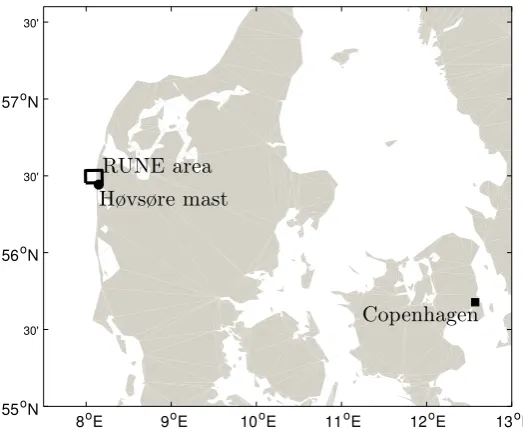
The RUNE near-shore experiment was conducted at the western coast of Denmark, as illustrated in Fig.1, on an area of about 9 km×5 km in the Lemvig municipality. A closer view of the area with the positions used for the installation of the lidars is shown in Fig.2.
8oE 9oE 10oE 11oE 12oE 13oE 55oN
30'
56oN
30'
57oN
30'
RUNE area
H
ø
vs
ø
re mast
Copenhagen
This area was selected because it is close to DTU’s test station of wind turbines at Høvsøre (position 2 in Fig.2is 6 km north from the test station’s main building), where we routinely perform wind-power measurements including those from a meteorological mast [14]. It is also a typical location of interest for offshore wind development. The site is well-serviced by a 4G network useful for device monitoring and data retrieval and needed for synchronization of the Windscanners.
The Høvsøre area is a nearly flat coastal farmland. A sand embankment separates the North Sea from the grasslands. Moving northwards, the embankment transforms into dune cliffs covered by grass. Close to position 3 in Fig. 2, the terrain is≈43 m above sea level (ASL). This is an important feature as lidars need a clear LOS to measure wind velocities and such topography aids in performing measurements over the North Sea with small elevation angles from onshore locations [15].
Figure 2. Topographic description of RUNE’s coastal experimental area based on a digital surface model (UTM32 WGS84, Zone 32V). The positions of the lidars are shown in different markers (see Table1for details). The colorbar indicates the height ASL.
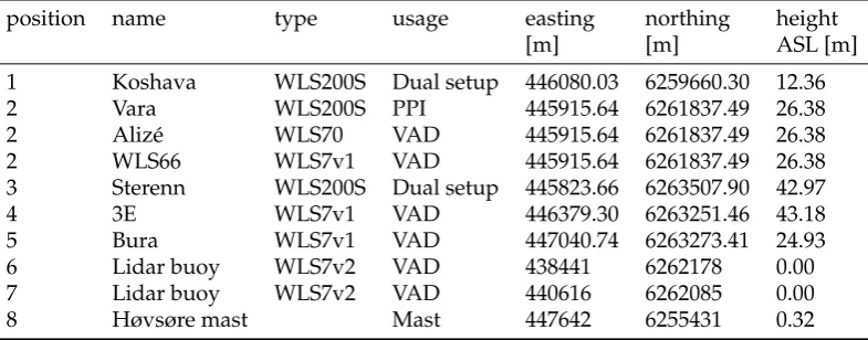
Table 1.Positions, coordinates (UTM WGS84, Zone 32V), types and main scanning strategies (usage) of the lidars during the RUNE campaign (see details in the text), including the information of the Høvsøre meteorological mast. The lidar buoy was used at two positions. The type is the commercial name given by the lidar manufacturer Leosphere.
position name type usage easting northing height
[m] [m] ASL [m]
1 Koshava WLS200S Dual setup 446080.03 6259660.30 12.36
2 Vara WLS200S PPI 445915.64 6261837.49 26.38
2 Alizé WLS70 VAD 445915.64 6261837.49 26.38
2 WLS66 WLS7v1 VAD 445915.64 6261837.49 26.38
3 Sterenn WLS200S Dual setup 445823.66 6263507.90 42.97
4 3E WLS7v1 VAD 446379.30 6263251.46 43.18
5 Bura WLS7v1 VAD 447040.74 6263273.41 24.93
6 Lidar buoy WLS7v2 VAD 438441 6262178 0.00
7 Lidar buoy WLS7v2 VAD 440616 6262085 0.00
8 Høvsøre mast Mast 447642 6255431 0.32
a lighthouse. The long-range profiling lidar Alizé and the short-range profiling lidar WLS66 were installed next to Vara. Two other short-range profiling lidars, 3E and Bura, were installed inland ≈250 m south, and≈550 and≈1200 m west of Sterenn, respectively. The location of the instruments was measured using a differential GPS system with an accuracy of≈10 cm. More information about the site identification for RUNE can be found in Courtney and Simon [15].
The topography of the area at a horizontal resolution of 1.6 m can be obtained via the website of the Danish Geodata Agency [16]. Land-cover data from the Corine dataset can be obtained via the website of the European Environmental Agency [17]. The land-use classes can be associated with an approximate surface roughness lengthz0by using Table 1 in Pindeaet al.[18]. The land-use classes
around the RUNE area are shown in Fig.3. The yellow area is associated with annual cropland (z0=
0.2 m). The villages of Bøvlingbjerg (≈3 km east of the Høvsøre meteorological mast) and Ramme (≈5 km east of RUNE’s experimental site) are the most prominent features that will impact the easterlies. The build-up areas showz0=0.8 m in the reclassified Corine data. The mixed forest area≈10 km east
of the site can also have an impact on the flow at high measuring heights during the campaign. Note that the roughness values that are discussed here are based on a simple reclassification of the land-use data, but Peñaet al.[14] found that the surface roughness at Høvsøre is much lower. They found that z0varies with season, direction, and atmospheric stability based on wind profile observations; the
all-sector long-termz0is 0.012 m. The differences between the Corine dataset-derived roughnesses
and the observed values is partly due to the applicability of the dataset; in mesoscale applications the roughness has to be representative for a grid cell of a kilometre or more, which is often bigger than the local roughness due to the non-linear impact of obstacles on the flow.
56.37°N 56.4°N 56.43°N 56.46°N 56.49°N 56.52°N 56.55°N 56.58°N
7.95°E 8°E 8.06°E 8.11°E 8.17°E 8.22°E 8.28°E 3
km
8
5
6
1
2
34
7
Continuous urban fabric Discontinuous urban fabric Industrial or commercial units
Road and rail networks and associated land Sport and leisure facilities
Non-irrigated arable land Pastures
Complex cultivation patterns
Land principally occupied by agriculture Coniferous forest
Mixed forest Moors and heathland Transitional woodland-shrub Beaches, dunes, sands Inland marshes Salt marshes Water bodies Coastal lagoons Sea and ocean
Figure 3.Land-use description of the terrain around the RUNE site. The main positions described in Sect.3are also given .
2.1. Timeline of the campaign
were prepared. During alignment and trajectory coding, all three Windscanners were used in a Plan Position Indicator (PPI) scenario at one elevation angle (see Sect.3.1for details). During this short phase the area experienced several winter storm events.
Phase 2 started on November 26, when Vara was setup in a PPI scenario at three elevation angles (Sect. 3.1), whereas Sterenn and Koshava follow trajectories in a synchronized manner, hereafter referred to as ‘dual setup’ (Sect.3.2). During a repair following a major hardware failure experienced by Koshava, the dual-setup trajectories were modified to reduce the spatial distance between range gates. This period is referred to as phase 3. Due to the hardware failure, the operational availability of both Koshava and Sterenn is low (see Table2).
During the final period, phase 4, Vara was setup in a PPI scenario covering an azimuthal angle of 120◦at an elevation angle of≈0◦. The two other Windscanners were used in a range height indicator (RHI) mode and because their trajectories were configured so that they matched at a point 5 km west of position 2, the matching vertical positions can be used as a ‘virtual’ mast (Sect.3.3).
3. Setup of the lidars
3.1. PPI scans
During phase 1, the three Windscanners performed PPIs covering an azimuthal range of 60◦with an elevation angle of≈1◦. The scans were centered at directions of 250, 270 and 290◦for Sterenn, Vara and Koshava, respectively. Each scan took 60 s to complete, i.e. the lidar was accumulating 1 s in each 1 degree azimuthal sector. There were 154 range gates for each LOS, except for Vara which had 156 range gates.
During phase 2 and 3 of the campaign, Vara was the only lidar performing 60◦PPI scans facing west but at three different elevation angles. These elevation angles were chosen such that the scans reach 50, 100 and 150 m ASL for a point 5 km west from position 2. An integrated velocity azimuth processing (IVAP) algorithm was used to reconstruct the horizontal wind components at each range gate. The IVAP algorithm uses a summation of the angularly separated LOS velocities [19].
During phases 2 and 3, the full trajectory was taking 145 s to complete; 45 s for each scan at the three different elevations and 10 s to travel back to the first measurement point. Each scan obtained 45 LOS velocities with 1 s accumulation time. Each LOS contained 156 range gates from 100 to 8150 m, so for each full scan 468 reconstructed horizontal wind components were obtained
During phase 4, Vara was performing a PPI scan with an azimuthal range of 120◦centered at 270◦. For each 1◦, the lidar was accumulating LOS spectra during 1 s. The elevation angle during this period was≈0◦and for each LOS there were 159 range gates.
The reconstruction algorithm described in Simon and Courtney [20] was applied to the PPI scans in phases 2 and 3 only (so hereafter PPI refers to such PPIs) for each scan and data were filtered out if the average carrier-to-noise ratio (CNR) of the 45 LOSs at each range gate was below−27 dB. The estimated wind components were then averaged over 10, 30 and 60-min periods, i.e. using 4, 12 and 24 reconstructed velocities per averaged value, respectively. In this article we only use the 10-min mean values.
3.2. Dual setup
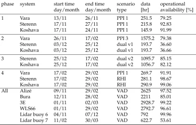
Table 2. Description of the measurement phases during the RUNE campaign. At each phase, operational availability is defined as the hours of acquired data divided by the amount of hours that the system could have acquired data. PPI 1 or 3 refers to scans with one or three elevation angles. v1 and v2 refer to the dual setup with the a larger and shorter distance between range gates, respectively.
phase system start time end time scenario data operational
day/month day/month type [hr] availability [%]
1 Vara 13/11 26/11 PPI 1 251.5 79.25
Sterenn 17/11 27/11 PPI 1 215.8 92.83
Koshava 17/11 24/11 PPI 1 145.9 91.99
2 Vara 26/11 17/02 PPI 3 1575.2 79.38
Sterenn 03/12 25/12 dual v1 193.7 36.60
Koshava 03/12 25/12 dual v1 193.7 36.66
3 Sterenn 25/12 17/02 dual v2 1095.7 85.15
Koshava 25/12 17/02 dual v2 1056.7 82.12
4 Vara 17/02 29/02 PPI 1 269.7 91.91
Sterenn 17/02 29/02 RHI 281.1 98.67
Koshava 17/02 29/02 RHI 290.9 99.06
All Alizé 09/11 29/02 VAD 2625 97.52
Bura 12/11 28/02 VAD 2211 85.01
3E 01/11 02/03 VAD 2928.7 99.22
WLS66 01/11 29/02 VAD 2792.7 96.61
Lidar buoy 6 04/11 07/12 VAD 792 99.96
Lidar buoy 7 11/02 30/03 VAD 622.7 53.61
reconstruction, 89 and 91 range gates were acquired per LOS and per system for phases 2 and 3, respectively.
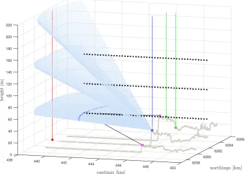
In order to include all acceptable range-gate combinations, a collocating algorithm filtered out data that did not fulfil a certain distance threshold, resulting in the black points depicted in Fig. 4. During phase 2, the range-gate positions were not well collocated in thex-direction (i.e. west–east), and therefore, the threshold in thex-direction was set to 51 m. For they(north–south) andz(vertical) directions and during phase 3, the threshold was 10 m. The reconstruction algorithm was applied to the 10, 30 and 60-min averaged LOS velocities of both systems, after filtering out data that did not fulfil the CNR threshold (−26.5 dB).
3.3. Virtual mast
During phase 4, Sterenn and Koshava performed RHI scans that intersected at a position 5 km west of position 2. A vertical profile with range gates at 36 different heights can be obtained (see Table3). For each 10-min interval, each height was sampled 16 times with 1 s accumulation time. Sterenn and Koshava had an azimuthal angle of 251◦and 293◦ and 143 and 144 ranges gates, respectively. They both swept an elevation range from ≈−0.5◦ to 9.5◦. The same reconstruction algorithm and CNR limit as those used for the dual setup were applied.
3.4. VAD scans
6266 6264 6262
northings [km] 6260
0 20 40 60 80 100
438 120
h
ei
g
h
t
[m
]
140
440 160
eastings [km] 180
200
442 6258
220
444 446 448
450
Figure 4.Overview of the scanning strategies during phase 2 and 3. Collocated points from the dual setup are shown in black circles and the two black lines show two laser beams focusing 5 km west of position 2. The points from the PPI scans are denoted with light blue points and dark blue points denote the first 60◦scan that is collocated with the first dual setup point at 50 m ASL. The green and blue lines denote the positions of the profiling lidars and the red line denotes the floating lidar buoy.
The sampling time per LOS was≈3.5, 1, 1, 5, and 1 s for Bura, 3E, WLS66, Alizé and the lidar buoy, respectively. All lidars were sampling in 4 positions around the zenith, with a 90◦azimuthal separation between each other. The zenith angle was 30◦ for the short-range lidars and 15◦ for the long-range lidar (Alizé). The CNR threshold for the VAD lidars was set to−22 dB, except for Alizé which used a threshold of−27 dB. All samples within a 10-minute period at all heights up to 130 m had to fulfill this threshold.
The lidar buoy was installed on November 4. On November 15, after a storm, it was found that the blades of the wind-power buoy generators were damaged and the buoy’s motion sensor was not working properly. During another storm, the blades were again damaged and the lidar did not have electricity after December 7. Due to the harsh weather conditions, it was only possible to relocate the
Table 3.The heights of the range gates of the VAD lidars and those of the virtual mast scenario.
name range gate height ALL [m]
Alizé 100,150,175,200,250,300,350,400,450, every 100 m from 500–1500 Bura 30,35,40,50,62,75,87,100,112,125,140,155,175,200,250,300
3E 40,57,70,88,107,125,150,200,250,300
WLS66 40,50,60,74,80,90,100,110,124,150
Lidar buoy 40,47,59,79,97,117,134,147,172,197,209,247
name Range gate height ASL [m]
buoy to a location with less-frequent breaking waves by February 11. There, the lidar buoy measured successfully until March 30. Detailed documentation about the lidar buoy can be found in [21].
4. Results
4.1. Wind climate
The RUNE campaign was characterized by periods of very windy weather with sustained winds from the west. Figure5-top panel shows the wind speeds from the cup anemometer at 100 m AGL at the Høvsøre meteorological mast. The wind speed at 100 m reaches more than 25 m s−1 several times, with a maximum wind speed of 35.3 m s−1 at 18:30:00 UTC on November 29. The wind direction (Fig. 5-bottom panel) is taken from measurements of a wind vane at 100 m AGL at the Høvsøre meteorological mast. These records show that the flow was characterized by westerlies during November and December and then a period of several weeks with mostly easterlies followed. After this intermezzo westerlies were again predominant.
10 20 30
December January February March
wind
sp
eed
[m
s
−
1]
NE E SE S SW W NW
December January February March
wind
direction
Figure 5. The wind speed (top panel) and the wind direction (bottom panel) at 100 m from measurements of the Høvsøre meteorological mast during RUNE.
4.2. Actual availability
The availability of measurements depends on the ability of the lidar to measure an accurate LOS velocity, which is mostly a function of the laser power and the presence of aerosols. We define ’actual availability’ when all samples within a 10-min interval fulfilled the thresholds discussed in Sect. 3 and a reconstruction of the wind vector could be obtained. Figure 6shows the actual availability of all lidars performing VAD, dual setup and RHI scans. It should be noted that only the PPI scans during phase 2 and 3 have been used to obtain reconstructed wind speeds.
gates fulfil that criteria are more rare. The lidar buoy was not available for a large portion of the experiment, but measured also during March. The other lidars only measured until February.
Dual setup Sector scan Aliz´e WLS66 Bura 3E Lidar buoy Mast
December January February March
Available Not Available
Figure 6.Actual availability of all reconstructed wind speeds in 10-minute intervals that fulfilled the filtering criteria
Figure7 shows the actual availability of the reconstructed horizontal wind speed components from the PPI and dual setup scans during phases 2 and 3 as a function of distance by assuming an operational availability of 100%. The actual availability decreases with distance (west–east) from the devices. The highest scanned points in the vertical coordinate, level 3, generally have the lowest availability. Further, availability from the dual setup is slightly lower than that of the PPI scan, because Koshava and Sterenn were located further away from the positions where the wind components are reconstructed compared to Vara (Fig. 2). The points over land with low availability are due to the laser beam hitting objects.
0 25 50 75 100
440000 442000 444000 446000
Eastings [m]
Av
ailabilit
y
[%]
dual setup 1 dual setup 2 dual setup 3 PPI 1 PPI 2 PPI 3
4.3. Preliminary intercomparisons
4.3.1. VAD lidars
In this section we use a data set which is the result of merging all lidars in VAD mode that fulfill the filtering criteria. Despite the CNR filtering, some data were found, where Bura measured near-zero wind speeds and 3E measured realistic values of more than 5 m s−1. These outliers were found within periods of near-zero temperatures (a comparison of Bura 10-min wind speeds with those from the Høvsøre meteorological mast at a similar level also showed these data). Therefore 10-minute intervals with an absolute difference of more than 5 m s−1between the wind from Bura
and 3E at 150 m were excluded. The result is a data set with 4640 10-min means.
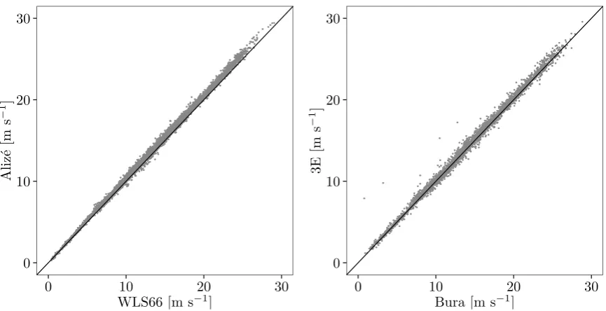
Figure8–left panel shows a scatter plot of the 126-m ASL 10-min mean wind speeds estimated from the collocated vertical profiling lidars WLS66 and Alizé, in order to get an idea of the quality of the data. The agreement is generally good (Pearson’s linear correlation coefficientR2is 1.00). Alizé
generally measures slightly higher wind speeds than WLS66 (≈3%). The mechanism responsible for this is yet unknown but it might be due to both the difference in the lidars’ measuring volumes (Alizé has a larger probe volume but measures over a smaller horizontal measuring area than WLS66) and the flow inhomogeneity near the cliff.
0 10 20 30
0 10 20 30
WLS66 [m s−1]
Aliz
´e
[m
s
−
1]
0 10 20 30
0 10 20 30
Bura [m s−1]
3E
[m
s
−
1]
Figure 8.Scatter plots of 10-min mean wind speeds at≈126 m ASL for WLS66 and Alizé (left panel) and at 150 m ASL for Bura and 3E (right panel). A line through the origin with a slope of 1 is shown in black
A similar comparison is illustrated in Fig. 8–right panel between 3E and Bura (at 150 m ASL), which are separated≈550 m, where the wind speeds are also in good agreement (1% bias andR2 =
0.99).
4.3.2. VAD and dual setup
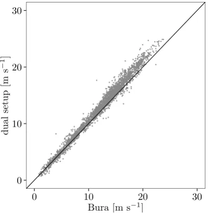
Figure9 shows the scatter plot for a height of 100 m ASL. Slightly more scatter can be seen compared to those in Fig. 8(6% bias andR2 = 0.98). This is also partly due to the effect of having only 4 samples in the dual setup, whereas Bura samples every 4 s within the 10-min intervals.
0 10 20 30
0 10 20 30
Bura [m s−1]
dual
setup
[m
s
−
1 ]
Figure 9.Scatter plot of the 10-min mean wind speeds for Bura and those reconstructed by the dual setup (for the positionx=447052 m) at≈100 m ASL. A line through the origin with a slope of 1 is shown in black
4.3.3. Dual setup and PPIs
There are only a limited amount of positions where the scanning patterns from the concurrent dual and PPI setups intersect and we expect differences in the estimated 10-min wind speed because of the difference in the size of the measuring volume, and the inherent spatial and temporal variability of the wind speed. The scanning pattern of both setups was chosen such that at 5 km west of position 2, they both measure at 50, 100 and 150 m ASL. Further, there are intersecting points at 50 m ASL, ≈0.9 and 1.7 km west of position 2.
Figure10shows scatter plots of the 10-min reconstructed mean wind speeds from the PPI and dual setup scans during phases 2 and 3. We only use data with 50% or higher actual availability within a 10-min interval to increase the number of 10-minute intervals that can be compared. The number of matching 10-min intervals is 4964, 4605, 1325, 1218, 1204 for Fig. 10panels a–e, respectively. Panels a and b show the wind speed at 50 m ASL at≈900 and 1700 m west of position 2, respectively. The agreement is good (R2=0.97 for both panels) but a cluster of points where the PPI scan shows higher
wind speeds is clearly seen. The mean bias is 0.1% and 0.8% for panels a and b, respectively.
Figure10(panels c–e) shows comparisons at 5 km west of position 2 at 50, 100 and 150 m ASL. The agreement is also good (R2=0.86, 0.88, and 0.83 for 50, 100, and 150 m ASL, respectively) and the mean bias is 2% for all heights. The lower agreement found compared to that of the positions closer to position 2 (in panels a and b) are most probably related to the assumption of flow homogeneity within the PPI scan that is needed for wind reconstruction, which is less valid when the PPI scan covers a larger area. At further distances there will be larger differences between the LOS velocities in a scan, due to the higher spatial separation. This makes it more difficult to reconstruct the wind speed. Furthermore, there can also be a bias due to a physical mean wind speed gradient present in the scanning area.
a)
0 5 10 15 20 250 5 10 15 20 25
dual setup [m s−1]
PPI
[m
s
−
1]
x=445011 m,z=50 m
b)
0 5 10 15 20 250 5 10 15 20 25
dual setup [m s−1]
PPI
[m
s
−
1]
x=444193 m,z=50 m
c)
0 5 10 15 20 250 5 10 15 20 25
dual setup [m s−1]
PPI
[m
s
−
1]
x=440921 m,z=50 m
d)
0 5 10 15 20 250 5 10 15 20 25
dual setup [m s−1]
PPI
[m
s
−
1]
x=440921 m,z=100 m
e)
0 5 10 15 20 250 5 10 15 20 25
dual setup [m s−1]
PPI
[m
s
−
1]
x=440921 m,z=150 m
deviation of the difference between the reconstructed wind speed from the dual and the PPI setups at 50 m ASL as a function of wind direction. The wind direction was determined from WLS66 at 76 m AGL due to its high actual availability and sorted into 30◦bins.
-3 -2 -1 0 1 2 3
0 90 180 270
wind direction [deg.]
dual
−
PPI
[m
s
−
1]
x=-1722 m x=-4994 m x=-904 m
Figure 11.The mean (marker)±standard deviation (error bars) of the difference between 10-min mean reconstructed wind speeds from the dual and PPI setups at 50 m ASL at three different westward positions. Thex-position is relative to the position of Vara with positive values going eastward.
From here on, we assume that there is no bias in the dual setup, because it needs fewer assumptions for reconstructing the wind speed. For the positions closest to coast (x = −904andx=-1722 m), the bias and standard deviation are highest for southerly winds (a mean bias of≈ 0.3 m s−1for the 180◦sector). For the point 5-km west from position 2, there is a bias in mean wind speed for the southerly and southwesterly winds of more than 1 m s−1. Very few samples are available for northerly winds, but a clear bias is observed for the furthest westward position. Further, the standard deviation in all direction bins is larger atx =−4994mthanatx=-904 m, which indicates that the reconstructed wind speeds show larger differences between the PPI and the dual-setup scans at large distances.
5. Conclusions and outlook
The RUNE campaign provides detailed novel measurements of the flow in the coastal zone. The flow during the campaign was mostly westerly, with higher wind speeds than usual in this time of the year and the occurrence of several storms. The availability of four land-based VAD lidars was the highest, generally above 95%. The PPI and dual setups showed a lower availability for longer ranges due to the decrease in backscatter signal. The virtual mast scenario had the lowest availability of the scanning setups because the wind speed is reconstructed 5 km from the coast. The power supply of the lidar buoy was damaged by waves several times and experienced long periods of unavailability.
speed reconstruction of the PPI scans for situations with low LOS velocities is expected and seen for northerly and southerly winds.
This preliminary analysis shows us the capabilities of the lidar measuring systems of RUNE. However, RUNE’s main scientific questions still remain to be answered and the next steps in our analysis will address them. First we need to find out what is the accuracy of flow models near the coast. This can be performed by evaluating mesoscale and microscale model outputs (and the combination of both) against RUNE measurements that also include the satellite and ocean buoy observations. We propose to construct blind benchmark cases based on RUNE’s measurements and distribute the description of the cases among the interested audiences. One of those works within the framework of the New European Wind Atlas (NEWA) project [22], in which the RUNE experiment plays an important role. Within NEWA, a number of modelers are going to evaluate the model results, which will be used to obtain the wind atlas, against high-quality measurements. Second we need to determine which is the best way to perform near-shore wind measurements in terms of accuracy, and economical and logistical feasibility. The dual setup and the PPI scans are the two options that can cover the area of interest; the dual setup needs two relatively expensive scanning lidars but the accuracy of reconstructed wind speeds is high because we do not need to assume horizontal flow homogeneity within the scanned area. The PPI scans can be performed by one scanning lidar, thus reducing costs and logistics, but we need to assume horizontal flow homogeneity within the scanned area, thus increasing the uncertainty. The question is whether the increase in uncertainty has a large impact when performing wind resource predictions and wind-power estimations.
Acknowledgments: Funding from the ForskEL program to the project ‘RUNE’ nr. 12263 and The European Commission partly funded ‘New European Wind Atlas’ project through FP7 are acknowledged. We would also like to acknowledge 3E for adding the 3E lidar to RUNE’s network, Fraunhofer IWES for the measurements from the lidar buoy, and the technicians of DTU Wind Energy, Fraunhofer IWES and the Danish Hydrological Institute for their work and support during the campaign
Author Contributions: M.C., G.L., A.P. and N.V. conceived and designed the experiments; G.L, N.V. and E.S. performed the experiments; R.F. analyzed the data; R.F. and A.P. wrote the paper.
Conflicts of Interest:The authors declare no conflict of interest.
References
1. Floors, R.; Vincent, C.L.; Gryning, S.E.; Peña, A.; Batchvarova, E. The wind profile in the coastal boundary layer: wind lidar measurements and numerical modelling. Boundary-Layer Meteorol.2013,147, 469–491. 2. Peña, A.; Gryning, S.E.; Hahmann, A. Observations of the atmospheric boundary layer height under marine
upstream flow conditions at a coastal site. J. Geophys. Res. Atmos.2013,118, 1924–1940.
3. Mortensen, N.G.; Heathfield, D.N.; Myllerup, L.; Landberg, L.; Rathmann, O. Getting started with WAsP 9. Technical Report Risø-I-2571(EN), Risø National Laboratory, Roskilde, Denmark, 2007.
4. Frank, H.P.; Rathmann, O.; Mortensen, N.G.; Landberg, L. The numerical wind atlas - the KAMM/WAsP method. Technical Report Risø-R-1252(EN), Risø National Laboratory, Roskilde, Denmark, 2001.
5. Landberg, L.; Myllerup, L.; Rathmann, O.; Petersen, E.L.; Jørgensen, B.H.; Badger, J.; Mortensen, N.G. Wind resource estimation - an overview. Wind Energy2003,6, 261–271.
6. Nunalee, C.G.; Basu, S. Mesoscale modeling of coastal low-level jets: implications for offshore wind resource estimation. Wind Energy2014,17, 1199–1216.
7. Badger, J.; Frank, H.; Hahmann, A.N.; Giebel, G. Wind-climate estimation based on mesoscale and microscale modeling: statistical-dynamical downscaling for wind energy applications. J. Appl. Meteorol. Climatol.2014,53, 1901–1919.
8. Smith, D.A.; Harris, M.; Coffey, A.S.; Mikkelsen, T.; Jørgensen, H.E.; Mann, J.; Danielian, R. Wind lidar evaluation at the Danish wind test site in Høvsøre.Wind Energy2006,9, 87–93.
9. Gottschall, J.; Courtney, M.S.; Wagner, R.; Jørgensen, H.E.; Antoniou, I. Lidar profilers in the context of wind energy – a verification procedure for traceable measurements. Wind Energy2012, 15, 147–159,
10. Pauscher, L.; Vasiljevic, N.; Callies, D.; Lea, G.; Mann, J.; Klaas, T.; Hieronimus, J.; Gottschall, J.; Schwesig, A.; Kühn, M.; Courtney, M. An inter-comparison study of multi- and DBS-lidar measurements in complex terrain. Remote Sens.,in review.
11. Vasiljevi´c, N. A time-space synchronization of coherent Doppler scanning lidars for 3D measurements of wind fields. Phd-thesis, Danish Technical University, Roskilde, Denmark, 2014.
12. Berg, J.; Vasiljevic, N.; Kelly, M.; Lea, G.; Courtney, M. Addressing spatial variability of surface-layer wind with long-range WindScanners. J. Atmos. Ocean. Technol.2015,32, 518–527.
13. Floors, R.; Lea, G.; Peña, A.; Karagali, I.; Ahsbahs, T. Report on RUNE’s coastal experiment and first inter-comparisons between measurements systems. Technical Report E-0115(EN), DTU Wind Energy, Roskilde, Denmark, 2016.
14. Peña, A.; Floors, R.; Sathe, A.; Gryning, S.E.; Wagner, R.; Courtney, M.S.; Larsén, X.G.; Hahmann, A.N.; Hasager, C.B. Ten years of boundary-Layer and wind-power meteorology at Høvsøre, Denmark.
Boundary-Layer Meteorol.2016,158, 1–26.
15. Courtney, M.; Simon, E. Deploying scanning lidars at coastal sites. Technical Report E-0110(EN), DTU Wind Energy, Roskilde, Denmark, 2016.
16. Geostyrelsen. http://download.kortforsyningen.dk/content/dhm-2007overflade-16-m-grid, Accessed on 2016-06-21.
17. EEA. http://www.eea.europa.eu/data-and-maps/data/corine-land-cover-2006-raster-3#tab-metadata, Accessed on 2016-06-21.
18. Pindea, N.; Jorba, O.; Jorge, J.; Baldasano. Using NOAA-AVHRR and SPOT-VGT data to estimate surface parameters : application to a mesoscale meteorological model. 1st Int. Symp. Recent Adv. Quant. Remote Sens.2002,1161, 16–20.
19. Liang, X. An integrating velocity–azimuth process single-Doppler radar wind retrieval method. J. Atmos. Ocean. Technol.2007,24, 658–665.
20. Simon, E.I.; Courtney, M.S. A Comparison of sector-scan and dual Doppler wind measurements at Høvsøre Test Station – one lidar or two? Technical Report DTU Wind Energy E-0112(EN), DTU Wind Energy, Roskilde, Denmark, 2016.
21. Gottschall, J.; Wolken-Möhlmann, G.; Viergutz, T.; Lange, B. Results and conclusions of a floating-lidar offshore test. Energy Procedia2014,53, 156–161.
22. Mann, J.; Angelou, N.; Arnqvist, J.; Callies, D.; Cantero, E.; Chávez Arroyo, R.; Courtney, M.; Cuxart, J.; Dellwik, E.; Gottschall, J.; Ivanell, S.; Kühn, M.; Lea, G.; Matos, J.C.; Veiga Rodrigues, C.; Palma, J.; Pauscher, L.; Peña, A.; Sanz Rodrigo, J.; Södeberg, S.; Vasiljevic, N. Complex terrain experiments in the New European Wind Atlas. Phil. Trans. R. Soc. A2016,in review.
c