Recreational Use Value of Lakes an Application of Travel Cost Method: A Case of Lake Ziway

http://www.sciencepublishinggroup.com/j/ijeee doi: 10.11648/j.ijeee.20190403.12

ISSN: 2575-5013 (Print); ISSN: 2575-5021 (Online)

Recreational Use Value of Lakes an Application of Travel

Cost Method: A Case of Lake Ziway

Yrgalem Desta

1

, Mekonnen Bersisa

2

1

Department of Economics, Faculty of Business and Economics, Raya University, Maichew, Ethiopia

2

Department of Economics, Faculty of Business and Economics, Addis Abeba University, Addis Abeba, Ethiopia

Email address:

To cite this article:

Yrgalem Desta, Mekonnen Bersisa. Recreational Use Value of Lakes an Application of Travel Cost Method: A Case of Lake Ziway. International Journal of Economy, Energy and Environment. Vol. 4, No. 3, 2019, pp. 56-62. doi: 10.11648/j.ijeee.20190403.12

Received: April 5, 2019; Accepted: June 12, 2019; Published: August 5, 2019

Abstract:

Lake Ziway is one of the largest fresh water Rift Valley Lakes of the Ethiopia; the Lake holds the intrinsic value and aesthetic quality of a wetland, including its functions like shelter for a diversity of plants, aquatic birds and fishes and it is also home of different monastery. This beautiful nature of the lake attracts many visitors. However, despite the many sources of attractions, because the public goods nature of the lake its demand and value in terms of its recreation service to society is not known, which makes deficit to sustain and expand the recreational service of the lake. For this reason this study analyzed the recreational value of Lake and its demand using an individual travel cost method (ITCM) based on face-to-face interview with 223 randomly selected local visitors of the Lake. The truncated Poisson model was used in the empirical analysis to estimate the recreational value of the lake and to identify its determinants. The econometric result of this model shows visitor’s martial statues, family size, and mode of transportation, type of visit, distance and travel cost are significant factors that affects the visitation rate for recreational site. And the study estimates that the on-site recreational benefits per visit per person was about 3353.64 per year and the expected total annual on-site recreational benefit of the site is 118,698,734.16 birr.

Keywords:

Individual Travel Cost Method, Truncated Poisson Model, Lake Valuation

1. Introduction

Lake Ziway is one of the largest fresh water Rift Valley Lakes of the Ethiopia, located 160 km far away from Addis Ababa in Oromia Regional State in Ziway town. It is a large open and shallow Lake with a catchment area of 6834 km2, a shoreline length of 137 km and a mean and maximum depth of 2.5m and 9m respectively. The Lake is known for its five bigger islands namely: Tulu Gudo, Tsedecha, Funduro, Debre Sin and Galila [1] and the Lake hold in excess of 20,000 birds; its avifauna is a major attraction to birdwatchers. The fish landing site in Ziway town attracts a number of fish eating birds including Great White Pelicans, White-breasted African Darter. Besides the interesting birdlife, the Lake also forms suitable habitat for Hippopotamuses [2]. Generally, the Lake holds the intrinsic value and aesthetic quality of a wetland, including its functions like shelter for a diversity of plants, aquatic birds and fish [1]. This beautiful nature of the lake attracts many visitors.

However, despite the many sources of attractions, because the public goods nature of the lake its value in terms of its recreation service to society is not known, which makes deficit to sustain and expand the recreational service of the lake. For this reason this study analyzed the recreational value of Lake and its demand using a travel cost method (ITCM).

2. Methodology

will overestimate the recreational value of the Lake and the estimated consumer surplus per trip will be bias [3]. In this regard it is expected that foreign visitors of Lake Ziway are MD and MP visitors. As a result this study used data only from local visitors as they tend to be single purpose (SP) and single destination (SD) visitors to estimate unbiased consumer surplus per trip (i.e. recreational benefit of the Lake). This would help to estimate nearly accurate recreational value and demand of the Lake, which are the main aims of this study.

The sample sizes calculated using the formula which is suggested by Kothari for finite population [4]. According to Ziway cultural and truism office average local visitors of the Lake are about 35,394 Visitors per year. Accordingly 223 local visitors of the lake randomly selected.

This study done based on analysis of travel cost method recreation value of Lake Ziway. The rationale behind this method is that, the time and costs which people are forgo to visit a place, indicates its recreational value. This method assumed that, the recreational value of a place reflected by the visitor’s total cost to visit it [5]. The travel cost method (TC), which is mostly relevant for determining recreational values related to biodiversity and ecosystem services. This method approaches the problems using either zonal travel cost method (ZTCM) or an individual travel cost method (ITCM). However, because individual travel cost method have several advantages over the zonal travel cost method, this study used individual travel cost method to estimate the recreational use value of the Lake.

And because of the data that used to estimate the recreational use value of Lake was collected only from visitors of Lake; Non-visitors will not be sampled, i.e. excluded from the study. Therefore, the application of Ordinary Least Square (OLS) to this type of data sets leads to biased estimates of the parameters. However, Maximum Likelihood estimation best suit these types of data sets, specifically count data models.

2.1. The Count Data Model

There have been numerous statistical methods that have been used to estimate single site demand models. The trip data is collected in the form of non-negative integers; this led to the use of count data models. According to Haab and McConnell, Count Data models are intuitively appealing for recreational demand because they deal with non-negative integer valued dependent variables. For recreation, the number of trips is a non-negative integer. The count model specifies the quantity demanded, trips, as a random non-negative integer, with a mean that is dependent on exogenous variables [6].

When we come to this study the estimation of the recreational value of the Lake, the dependent variable number of visits assumes only integer values that are greater or equal to one (nonnegative). Hence count data models are a good fit for this study.

The basic count model is written

( _{i j} ) ( , _i )

p r V = n = f n z

β

(1) Where Vij is individual i’s visit to site j and n=1, 2, 3……

This study used the Truncated Poisson Model (TPM) than different count data models for estimating the recreational demand of Lake because there is no a problem of over dispersion.

The following truncated model is adapted from Green with some adjustment to recreation sites [7].

Consider the trip generating function of an individual travel cost method as

'

= + i

Vij

β

X

ε

(2)

Where

2

Xi (0, )

ij N

ε

≈

δ

and assume that

(

)

Vij Xi≈N µ,δ2 ;µ=β'Xi (3) Where Vijis individual i’s visit to site j, β'Xi is the deterministic part of the classical regression model, specifically

x

i

is vector of explanatory variables,

β

is a

parameter and

ε

i is an error term. With truncated sampling,

we observe Vij only if Vij >1. This indicates that 1

X

β

+ ≥

ε

. Given that Vij is truncated from below at Vij>1. If

( )

Vij has normal distribution with mean µ and standard deviationδ , then

ij

1 µ

prob(V 1) 1 Φ 1 Φ(α)

σ

−

 

> = −  = −

  (4)

Where

α

1

µ

σ

−

 

= 

 and Φ

( )

. is the standard normal CDF.

The density of the truncated normal distribution is then

(

)

f Vij

( )

( )

f Vij Vij 1

prob Vij 1

≥ =

≥ (5)

(

)

( )

Vij βX 1

φ .

δ δ

1 Φ αi

 ₋ 

 

 

 

= −

(6)

Where ϕ

( )

. is Standard normal pdf. Following this the mean will be as follow

(

)

(

(

1 β'X /δ

(

(

)

)

)

)

E Vij Vij 1 β' δ

1 Φ 1 β'X δ −

≥ = +

− − (7)

There is similar attenuation for the variance. In the condition y>1, the variance is not σ2 rather;

(

)

2

(

( )

)

Var Vij Vij 1≥ =δ 1 σ α− (8) In this study the estimation of the recreational value of the Lake, the dependent variable number of visits assumes only integer values that are greater or equal to one (non-negative). Hence count data models are a good fit for this study. This study used the Truncated Poisson Model (TPM) rather than Truncated Negative Binomial Model for estimating the recreational demand of Lake because there is no a problem of over dispersion. The Poisson model is best suited for distributions that are free from over dispersion when variance and conditional mean of the number of visits are equal (equi-dispersion). However, for count data the variance usually exceeds the mean, a feature called over-dispersion. In such case the conditional mean will incorrectly specified, which leads to the more fundamental problem of inconsistency and inefficiency of maximum likelihood estimation [8]. So, if such a problems exist Truncated Negative Binomial Model would be best than Truncated Poisson Model for estimating the recreational demand of Lake. However, in our data there is no problem of over dispersion is Truncated Poisson Model (TPM) used.

The Poisson probability density function is given by

Pr( )

!

−

= = in

ij

e

v n

n

λ_λ

(9)

Where, n = 0, 1, 2... N, and the parameter

λ

i is both the

mean and the variance of the distribution. When the first two moments of this distribution are equal each other

( [E v_ij]= =λ Var v[ _ij] ), known as equi-dispersion. This model can be extended to a regression framework by

parameterizing the relation between the mean parameter λ and a set of explanatory variables X.

Where,

λ

_i =exp( ' )x

β

i=1… n

Where X is the matrix of K explanatory variables and β is a conformable matrix of coefficients to be estimated. Given the above two equations, the Poisson regression model can be estimated, under the assumption that v_ij/x_iare independent, by maximum likelihood.

2.2. Functional Forms of ITCM

In empirical estimation of recreation demand models, several functional forms have been used. The most popular functional forms are linear, quadratic, semi-log and log-log. Economic theory does not suggest any particular functional form for TCM [9]. In this study semi-log functional form used because it simple and convenient to estimate consumer surplus per visit and the recreational benefit obtained from the Lake.

(10) Where

Vi = Number of visits taken per year by individual i to Lake Ziway.

TCi = Visit cost faced in birr by individual i to Lake Ziway.

Xi = All other factors determining individual i's visits (socio-economic characteristics)

In this study the specific econometric model that used to describe the relationship between individual visits per year and the travel cost and other explanatory variables is given as:

Visitation rate =f (travel cost, age, sex, education, family size, marital status, visitor occupation, distance in hour, type of visitation, income, mode of transportation)

0 1 2 3 4 5 6 7 8 9 10 11

i i

V =β +βTC+β GEN+β AG+β MRS+β FS+β EDU+β INC+βTYVI+β MOTR+β EMC+β DC+ε (11)

Where: V= Individuals' number of visits. TC = visitors' travel cost.

AG = visitors' age.

GEN= visitors' gender as dummy variable MRS = visitors’ marital status as dummy variable FS = visitors' family size.

EDU = visitors' level of education in year INC= visitors' monthly income in birr1 TYVI = type of visit in a group or alone MOTR = visitors' mode of transport EMC = visitors employment characteristic DS=distance from Lake Ziway to home in hour

Β0, β1, β2, β3, β4, β5, β6, β7, β8, β9, β10, β11 and β12 are the parameters and ε i = error term.

1 Birr is Ethiopia national currency

(

TC i Xi

)

F

3. Results and Discussions

3.1. Descriptive Statistics

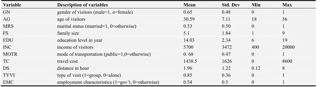
Table 1. Visitors socio economic and demographic characteristics.

Variable Description of variables Mean Std. Dev Min Max

GN gender of visitors (male=1, o=female) 0.65 0.48 0 1

AG age of visitors 30.59 7.11 18 56

MRS marital status (married=1, 0=otherwise) 0.53 0.50 0 1

FS family size 5.1 1.84 1 9

EDU education level in year 14.03 2.34 6 19

INC income of visitors 5700 3472 400 20000

MOTR mode of transportation (public=1,0=otherwise) 0. 68 0.47 0 1

TC travel cost 1438.5 1626 0 8600

DS distance in hour 1.96 1.22 0.12 8

TYVI type of visit (1=group, 0=alone) 0.85 0.36 0 1

EMC employment characteristics (1=gov’t, 0=otherwise) 0.54 0.5 0 1

Source: own survey, 2017

**Note that the mean estimates of dummy variables should be interpreted as percentage. For example the mean of the respondents’ sex is 0.6457. This means that 65% of the respondents are male.

3.2. Econometric Analysis and Regression Results

In the econometric analysis different socioeconomic and demographic variables that are expected to explain the dependent variable are included. In this study, a log-linear functional form for the demand function is used.

Therefore, the demand function for the Lake Ziway outdoor recreational site has the following form

0 1 2 3 4 5 6 7 8 9 10 11

lnV_i=β +βTC+β GEN+β AG+β MRS+β FS+β EDU+β INC+βTYVI+β MOTR+β EMC+β DC+ε_i (12) In this study because the dependent variable number of

visits assumes only integer values that are greater or equal to one (non-negative). Hence, count data models are a good fit for this study. For this reason a count data model used for the econometric analysis. Among the different count data models the truncated Poisson regression Model (TPM) is employed because of its suitability for this study’s data. The TPM is preferred because the data that use in this study not have a problem of over dispersion. Over dispersion appears when very few people make higher number of visits and the majority makes very few trips [8]. This is reflected by a higher variance of the number visits than the mean number of

visits of sample visitors. In fact in this study the variance is found to be 0.74 that is lower than the mean which is 1.98 for the number of trips. Therefore, the data is free from the problem of over dispersion. So, truncated poison model (TPM) is the appropriate model for the analysis rater then the negative binomial model.

Because there are some visitors who made only one trip and if one trip is not added to these values its logarithm will be zero and which cannot be computed using truncated count data model. Therefore, for computational reason one trip is added to all visitors which is (V 1)_i+ =vi

So, the above function becomes as follow;

0 1 2 3 4 5 6 7 8 9 10 11

lnv_i =β +βTC+β GEN +β AG+β MRS+β FS+β EDU+β INC+β TYVI+β MOTR+β EMC+β DC+ε_i (13)

Where (V 1)i+ =vi

To test the significance of the truncated poison model (TPM) regressions to this study the log-likelihood ratio test, the pseudo-R2 value and the Akaki information criteria (AIC) and Bayesian Information criteria (BIC) are used.

The pseudo R2 for truncated Poisson model is 26.75% is better than other count data models and the overall significance of the model was tested using the log likelihood ratio test. The log likelihood ratio calculated as;

LR= -2(Restricted Log-L – Unrestricted Log-L)

In this study the restricted log likelihood is -282.75 while the unrestricted log likelihood is -213.73, thus the LR is equal to 69. The critical value of the chi-square distribution for 11 degrees of freedom at 1 percent is found to be 24.72.

The calculated value is higher than the tabulated value at one percent significant level. Therefore, the null hypothesis that all the explanatory variables are irrelevant in the determination of the variation in the dependent variable can be rejected at 1 percent level of significance. This implies that the estimated model exhibits an overall significance.

The Akaki information criteria (AIC) and Bayesian Information criteria (BIC) for truncated Poisson regression model is low as comparing to other count models, which shows that the Poisson regression model is better model for estimation than any other models.2

3.3. Determinants of Recreational Demand (Visitation) of the Lake

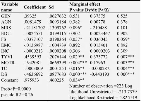
Number of people visiting (visitation rate) a recreation site is affected by number factors such as socioeconomic and demographic characteristics of the visitor’s and the travel cost associated with trip to the recreation site. The sign, magnitude and level of significance of the estimated parameters of the determinants of visitation rate visitors are discussed here from the below table.

Table 2. Robust regression result of the Truncated Poisson regression.

Variable

name Coefficient Sd

Marginal effect P value Dy/dx P>/Z/

GEN .39325 .0627632 0.531 0.37375 0.525

AGN .0081479 .0093184 0.382 0.00778 0.378

MRS -.21181702 .1309762 0.096* -.210488 0.101

EDU -.0024551 .0199115 0.902 0.0023467 0.902

FS -.0377107 .0198364 0.057* 0.036045 0.059*

EMC -.0136987 .1004739 0.892 0.013401 0.892

INC -.0000213 .0000208 0.306 0.0000203 0.309

TYVI .4539593 .2076144 0.029** 0.373772 0.007***

MOTR .1942081 .0669399 0.004*** 0.17963 0.003***

TC -.0003009 .0001254 0.016** -0.000287. 0.004***

DS -.4636692 .0877683 0.000*** -0.443193 0.000***

Constant .975933 .460225 0.034**

Prob>F=0.0000 pseudo R2 =0.26

Number of observation =223 Log likelihood Unrestricted = -213.7379 Log likelihood Restricted = -282.7519

Source: own survey, 2017.

***, ** &* represent statistically Significant at 1%, 5% and 10% level of significant, respectively.

The travel cost (TC) which is the sum of all travel cost expenses including the travel time cost. The travel cost was expected to have a negative relation with the number visitation to Ziway Lake recreation area. As expected the result from our study showed the expected sign in coefficients, negative sign and is significant at 5% significance level; which specifies that when the price of goods/service (travel) increases then the demand of the good/service (i.e. number of visits) will decrease. The coefficient of the travel cost shows that other things remain constant, a one birr increment in the travel cost will decrease the number of visits made to the site approximately by 0.02876%. This means that people living closer to the site made many trips while those living far from the site made fewer trips because travel cost for them is relatively low.

Distance (DS) of the visitor’s resident from the Lake was expected to have a negative relation with the respondent’s visitation rate. As expected the result from this study shows the distance of the respondents from the Lake have a negative sign with 1% significant level. The coefficient distance shows that other things remain constant, a one hour increment in the distance between the Lake and the respondent resident will decrease the number of visits made to the site approximately by 44.31%. This means that people living closer to the site made many trips while those living far from the site made fewer trips.

The family size (FS) was expected to have a negative

relationship with respondents’ visitation rate. As expected the result from this study showed that expected sign at 10% level of significance. The coefficient of this variable shows that other things remain constant a one person increase in the family member of the respondent will decreases the number of visits made to the site approximately by 3.604%. This implies that people who have few family members made many as comparing to peoples who have large family size.

A dummy variable coefficient represents to the marital status (MRS) of the visitors, which is 1 married visitor and 0 otherwise, was expected to have a negative relationship with the respondent’s visitation rate. As expected the results from this study shows that the marital statuses have a positive sign with 5% significant level. The coefficient of this variable shows that other things remain constant; married visitors have 21.04% less probability of visiting the Lake than the visitors who are not marred.

A dummy variable coefficient represents to the type of the visitation (TYVI), which is 1 for group visitors and 0 otherwise, was expected to have a positive relationship with the respondent’s visitation rate. As expected the result from this study shows that the visitation characters have a positive sign with 5% significant level. The coefficient of this variable shows that other things remain constant; visitors who visit the Lake in group have 37.37% probability of visiting the Lake than the visitors who visit the Lake lonely.

A dummy variable coefficient represents to the mode of transportation (MOTR) used by the visitors to reach Lake Ziway, which is 1 for public transportation (including walk) and 0 otherwise, was expected to have a positive relationship with the respondent’s visitation rate. As expected the results from this study shows that the mode of transportation has a positive sign with 1% significant level. The coefficient of this variable shows that other things remain constant; visitors who use public transportation to visit the Lake have 17.96% more probability of visiting the Lake than the visitors who use other transportation method. This is may be due to the reasons that visitors who us public transportation spent low travel cost than those visitors who use other transportation method.

The variables of gender, employment characters and age have the expected sign. However, they are insignificant.

3.4. Estimation of the Demand for the Recreational Value of the Lake

This study uses the estimated coefficient of travel cost to calculate the recreational benefit and consumer surplus of the Lake to the visitors. Basically there are two steps to reach at the final welfare of the visitor. The first step is estimating the demand relationship for the recreational benefit. This demand function can be estimated by using the coefficients the mean values of significant variables i.e. this is done by relating the number of visit with the travel cost.

The linear semi log demand function is as follows: Functionally,

i 0 1 i

Where; v_i refers the visitation rate TC refers the travel cost of trip

i

ε

refers to the stochastic error term and

β

₀and

β

₁ are parameters

The estimated Marshillian demand function for Lake Ziway can be written as:

i

lnv =0.976 .0002876TC− (15)

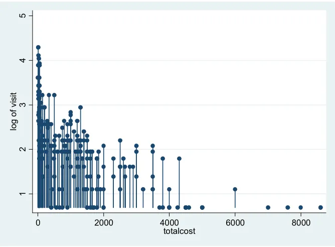
Figure 1. Estimated scattered individual recreational demand curve of Lake Ziway.

Figure 1indicates that the estimated demand curve for the recreation in the Lake is downward sloping, i.e. as a travel cost increases the number visitation to the lake decrease; this fits with the theory of demand.

The second step is the estimation of the annual recreational benefit of the Lake recreational site per person and then to aggregate, it is important first of all to transform the above demand function in to its inverse form. When the above demand function is transformed, then the area under the demand curve is the recreational benefit of the site. This calculated by integrating the inverse demand function between zero and mean trip of 1.98. Accordingly, the estimated recreational benefit for the average number of visits is birr 8901. Therefore the recreational value of the Lake per visit per person is estimated to be approximately 4495.5 birr.

The annual total recreation value of the Lake is calculated by multiplying the number of visitors registered within a year and recreation benefit person per visit. According to Ziway cultural and truism office average local visitors of the Lake are about 35394 Visitors. Therefore, total recreation values of the Lake become;

Total annual recreation benefit

4495.5*35394=159,113,727 birr

But this value is all round values related to outlays made from the start of the trip to the Lake and up to the trip made back to home from the Lake. So, all of this recreational benefit cannot be attributed to the on-site experience. Hence,

we need to find a technique to evaluate how much of this benefit gained purely related to the on-site experience. The common method is asking visitors to allocate percentage points to the on-site and off-site experience to evaluate how much of the utility of the whole recreational experience is due to the on-site experience [10]. In this study a similar procedure was followed, i.e. visitors were asked to allocate their total enjoyment in on-site experience as comparing to off-site enjoyment. According to respondents’ response about their utility proportion to the onsite benefit of Lake Ziway recreational site relative to the offsite, about 74.6% of enjoyment belongs to the onsite recreation. By taking this information, on-site recreational benefit per visit per person estimated by multiplying the percentage enjoyment being on on-site with the estimated benefit of the recreational value of the Lake per visit per person. Therefore, the on-site recreational benefit per visit per Person found to be;

4495.5 * 0.746 = 3353.64 birr

And the aggregate annual on-site benefit for the total numbers of annual visitors of the Lake found to be;

3353.64*35,394 = birr 118,698,734.16birr

Consumer surplus is a widely accepted measure of net social benefit. It represents the difference between an individual‘s willingness to pay and actual expenditure for a good and service. Using the exponential demand function, consumer surplus (CS) for the average number of visits is calculated as the area below the demand curve and above the

1

2

3

4

5

lo

g

o

f

v

is

it

0 2000 4000 6000 8000

average travel cost of birr 1438 or the estimated coefficients can be used to calculate the consumer surplus per predicted trip defined as;

1/

−

β

Tc (16) Where βTC is a coefficient of the travel cost variable Using the above formula Thus, individual consumer surplus (CS) per visit found to be 3477 birr i.e. CS= (1/-0.0002876). And the average recreational value per person is calculated by dividing the average consumer Surplus per visit to the average number of visit per year. Therefore, the average consumer surplus per visit per person is equal to birr 3477 /1.98= 1756 birr.

The annual total (aggregate) consumer surplus per visit was calculated by multiplying the annual average number of visitors of the Lake by the average consumer surplus per visit per person, which was approximated to Birr 62,154,928 birr.

4. Conclusion

The study estimated the recreational value of the Lake Ziway using individual travel cost method based on face-to-face interview with 233 randomly selected local visitors of the Lake. For this study individual travel cost method was used because it has several advantages over zonal travel cost method. The survey results obtained from this individual travel cost method analyzed by using both descriptive and econometric analyses. Since the data for the dependent variable (visits per year) are count data (integer), count data models were used. The dependent variable is truncated at a point where number of visits is greater than or equal to 1. Furthermore the statistical test showed that the data has no over dispersion problem. Thus, the truncated Poisson model was used in the empirical analysis instead of the negative binomial model and other count models.

The result from the Truncated Poisson regression shows that six variables were achieved the expected sign and significant in deferent level of significances in determining the visitation rate for recreational site. These are visitor’s martial statues, family size, and mode of transportation, type of visit, distance and travel cost. The explanatory variables sex and employment type achieved the expected sign but they are insignificant. Conversely the variable age, education and income has unexpected sign and insignificant.

The study estimated that the individual outdoor recreational demand for the Lake;

i

lnv =0.976 .0002876TC− (17)

The recreational benefit computed from the regression analysis indicated that the on-site recreational benefits per visit per person was about 3353.64 birr per year and the expected total annual on-site recreational benefit of the site was 118,698,734.16 birr. And the average consumer surplus per visit per person and the annual total (aggregate) consumer surplus per visit was found to birr 1756 birr and 62,154,928 birr respectively.

Decision makers including Policy makers have no idea as to the economic values of environmental resources such as a recreational value of this lake. They base their decision on their value judgment. This makes deficit to sustain and expand the recreational service of the lakes. Therefore, they should make their decisions based on estimates obtained through valuation techniques.

References

[1] Petra S. et.al. (2009). Past, Current and Potential Production of Fish in Lake Ziway. Wageningen International.

[2] EWNHS. (2010). A Glimpse at Biodiversity Hotspots of Ethiopia. Ethiopian Wildlife & Natural History Society (EWNHS).

[3] Loomis J., Yorizane S., and Larson D.,. (2000). Testing Significance of Melti Destination and Multipurpose Trip Effects in a Travel Cost Method Demand Model for Whale Watching Trips. Agricultural and Resource Economics Review.

[4] Kothari C. (2004). Reserch Methodology: methodes and techinues. New Delhi: New Age International.

[5] Amirnejad H. et.al. (2011). The Comparison of Contingent Valuation and Travel Cost Method in Estimation of Economic Value of Recreational, Tourism and Aesthetic Functions. [6] Haab C. and McConnell E. (2002). Valuing Environmental

and Natural Resources; Econometrics Of Non-Market Valuation. Edward Elgar Publishing Limited.

[7] Greene H. (2003). econometic Analysis. new jersy: Pearson Education LTD.

[8] Cameron C. and Trivedi K. (2005). Microeconometrics Methodes and Applocations. new york: Cambridge University Press.

[9] Himayatullah K. (2006). Willingness to Pay for Margalla Hills National Park: Evidence from the Travel Cost Method. The Labore Journal of Economics.