Comprehensive Bayesian structural identification using
temperature variation
Andre Jesusa,∗, Peter Brommerb,c, Yanjie Zhua, Irwanda Laorya,∗
aCivil Research Group, School of Engineering, University of Warwick, Coventry CV4 7AL
UK
bWarwick Centre for Predictive Modelling, School of Engineering, University of Warwick,
Coventry CV4 7AL, UK
cCentre for Scientific Computing, University of Warwick, Coventry CV4 7AL, UK
Abstract
A modular Bayesian method is applied for structural identification of a reduced-scale aluminium bridge model subject to thermal loading. The deformation and temperature variations of the structure were measured using strain gauges and thermocouples. Feasibility of a practical, temperature-based, Bayesian struc-tural identification is highlighted. This methodology used multiple responses to identify existent discrepancies of a model, calibrate the stiffness of the bridge support and establish uncertainty of a predicted response. Results show that the inference of a structural parameter is successful even in the presence of sub-stantial modelling discrepancies, converging to its true physical value. However measurements should have a high dependency on the calibration parameters. Usage of temperature variations to perform structural identification is high-lighted.
Keywords: Bayesian inference, model calibration, structural-identification, identifiability, temperature variation
1. Introduction
The capability of a structural health monitoring (SHM) system to interpret monitored data is the main factor that dictates its performance and its usefulness to owners and local authorities.
Interpretation of the data using a physics-based model is advantageous be-cause its development and usage as a predictive tool agrees with engineering knowledge, making it more understandable. However the main disadvantage is that the model has to be calibrated, before it can be used as a predictive tool. Moreover, using a deterministic model, i.e. a model where input parameters and
∗Corresponding author
response outputs are deterministic, rarely correlates well with real data, due to the complexity and inherent uncertainties of this latter one. Hence in most sit-uations a probabilistic approach is more realistic [1] and methods such as model falsification [2], fuzzy numbers [3], Kalman filters [4], sampling methods [5], Markov processes [6] amongst others [7] have been developed for this purpose.
Bayesian inference is the basis of a class of well known methods which also allow to perform structural identification. Beck [8,9] is known as one of the pio-neers of the application of Bayesian methods in SHM. Numerous research works have been conducted on the basis of this initial framework [10,11]. Based on this research, two fundamental problems might be thought as to why Bayesian meth-ods were not widely applied in SHM practice. Firstly, the model parameters to be calibrated are often assumed as fixed physical properties of the infrastructure, while in reality these properties change due to external factors such as traffic and environmental variations [12], e.g. stiffness of the structure. Secondly, un-certainties due to modelling errors are only partially considered, despite being ubiquitous. They can be caused by: (a) discrepancy between the behaviour of a physics-based model and that of the real structure; and (b) numerical error in solving the partial differential equations (e.g. finite element method and mesh discretization). Component (a) is extremely difficult to quantify. Most of the present research [13,14] usually disregard this form of uncertainty or consider it as zero mean Gaussian distributed [6]. Only a limited number of authors in the SHM community, namely Higdon [15] and Simoen [16] have applied Bayesian methodologies under this scope. Model-based Bayesian structural identification with temperature variations is also considerably scarce in the literature [17,12]. Higdon applied a comprehensive modular Bayesian method originally devel-oped by Kennedy and O’Hagan (KOH) [18,19], which was not widely accepted, presumably because of a lack of identifiability [20, 21]. Identifiability is un-derstood as the capability of inferring the true value of model parameters that represent a physical property, e.g. Young modulus, based on available data. Arendt et al. [22] suggested an improvement to the KOH original formulation to solve the identifiability problem, by using monitored data with diversified responses. This approach was validated on a simulated simply supported beam. We believe that this formulation is very comprehensive to quantify existent uncertainties and superior in some aspects to the ones used in previous works.
Based on this resurgent interest of the modular Bayesian method, the present work focus on its practical application for structural identification using thermal variations. Studies on advantages of using temperature loading for structural identification can be found in the works of Laory [23, 24] and Yarnold [25]. The objective at hand is to test the performance of the improved algorithm on a scale aluminium bridge model subject to thermal loading. To the best of our knowledge this test is the first practical application of this methodology, particularly for temperature based structural identification.
scenarios; damaging the structure is permissible and allows to easily test damage identification methodologies.
This paper is organised as follows: In section2, a description of the model calibration formulation is given; section3 describes the aluminium bridge and its finite element (FE) model, presents a sensor placement analysis, application of the method and its results, and finally, section4 highlights the conclusions of the present work.
2. Model calibration formulation
This section describes the model calibration approach. A more detailed description can be found in [22]. An introduction to Gaussian process emulation is presented in Appendix A. An outline of the general formulation is given in the next subsection followed by a brief overview of the algorithm and of the numerical approach. To a more in depth description of the uncertainties considered by this methodology see Section 2 of [20].
2.1. Observation and numerical model equations
Let us now assume that a given continuous process ξ has n observations ofq responses Ye and is dependent onddesign variables Xe. Its observation equation can be written as
Ye(Xe) =ξ(Xe) +ε (1)
where εT = [ε
1, . . . ,εn] is an observation error that is assumed to follow a Gaussian distribution N(O,Λ). On the other hand the unobservable process
ξ(Xe) is described using a numerical model Ymas follows
ξ(Xe) =Ym(Xe,θ∗) +δ(Xe) (2)
where δ(Xe) is a discrepancy function that translates the difference between the model and the true process,Ym(Xe,θ∗) is the model output andθ∗ are a r-dimensional vector of structural parameters. This equation is an ideal state of the model (i.e. the model is successfully calibrated) when the model parameters
θ take the values θ∗. Although our example updates only one parameter, the methodology can also consider multiple parameters, which is a common scenario in civil infrastructures [26, 27,13].
It is important to mention that the discrepancy function is independent of the model output and is an unknown of the problem as well as the structural parameters. Now substituting equation number2 in equation number1 results in
The numerical model and the discrepancy function shall now be replaced by multiple response Gaussian processes (mrGp), whose hyperparameters have to be determined (see the Appendix for a definition and details). These hy-perparameters characterise the mrGps and account for an approximation of its associated uncertainties, such as: variability of the numerical model; modelling discrepancies and observation error.
One way of determining the hyperparameters is by applying a Bayesian ap-proach, which fully accounts for all the considered uncertainties and determines all the hyperparameters at the same time. However this implies a significant computational effort and is not recommended [28]. Instead a modular Bayesian approach shall be used, and is described in the following section.
2.2. Modular Bayesian approach
A modular Bayesian approach (MBA) separates the calibration process into four modules, on which the mrGp hyperparameters are estimated separately and progressively [29] as detailed in Fig.1 (based on Fig. 5 from [20]).
Fixing the hyperparameters at an estimated value reduces the degree of approximation of the uncertainties covered by the mrGp. By doing so, the ‘second order’ effect of those uncertainties is being neglected. This means that preference has been given to recognise all of these sources of uncertainty, to a certain extent at a lower computational cost, rather than fully accounting for the uncertainties, with a considerable increase of computational effort.
Module 1: Gaussian Process for numerical model
Replace the numerical model with a mrGp model Simulation Data(Xm,Θm), Ym
Output: Hyperparametersφm
Module 2: Gaussian Process for discrepancy function. Replace the discrepancy function with a
Module 3: Posterior of the calibration parameters Use Bayes theorem to calculate the posterior
p(θ|d,φˆ) =p(d|θ,φˆ)p(θ)/R
p(d|θ,φˆ)p(θ)dθ
Output: Posterior ofθ
distribution for the calibration parameters
MeasurementsXe, Ye
Module 4: Prediction of the experimental response and discrepancy function
ye(x)|θ,φˆ∼mrGp(me(·), Ve(·,·))
Output: Prediction of experimental Output: Hyperparametersφδ
response and discrepancy function
Prior of the calibration parametersp(θ) mrGp model.
This act of estimating and fixing the hyperparameters is applied progres-sively, when moving from module 1 to module 2 and from module 2 to module 3. Estimation is done with numerical optimisation methods by maximising the likelihood between the mrGp and the available data.
In our case we used a matlab genetic algorithm (GA) routine. An initial population of size 40 was generated in the [0–1] range, with default values for Gaussian mutation function (mean 0, standard deviation 1 and shrinkage of the standard deviation as generations go by 1) and scattered crossover function (0.8 fraction of the population at the each next generation). Convergence criteria are set as either a maximum number of 100 generations or an average change in the fitness value less than 1×10⁻⁶.
It is important to stress that the discrepancy function is not being updated i.e. it is not the same as a GA fitness function. Instead the GA in module 2 (see Fig.1) aims to estimate the parameters of a statistical model (a Gaussian process), that approximates the discrepancy function. This is done through maximum likelihood estimation (MLE), which implies that the fitness function of the GA is the likelihood function.
In module 3, Bayes’ theorem is used for approximating the posterior distri-bution ofθ. In contrast to other approaches mentioned in the introduction, its likelihood function contains the two mrGp approximated in modules 1 and 2, now with its hyperparameters fixed.
3. Aluminium bridge subjected to thermal loading
In this case-study a reduced-scale laboratory aluminium bridge inspired by the New Joban Line Arakawa (Japan) railway bridge, was built at the War-wick Civil Engineering Laboratory and subjected to thermal loading due to infrared heaters. Typical daily ambient temperature in the laboratory ranged from 291.15 K up to 294.15 K. A numerical model of the structure was also developed to study the phenomena. The stiffness of a pair of springs located at one of the ends of the bridge will be considered as a model parameter to be calibrated. Subsection3.3details a combinatorial analysis to select the best out of a set of available inputs, to maximise the performance of the method, which is subsequently applied and results are shown in subsection3.4.
3.1. Experiment
The truss structure in Fig.2(a)is simply supported at its ends, being con-strained on one of them by two linear springs Fig.2(b)(supplier reference value isK= 552.26 N/mm).
(a)
(b)
Figure 2: Aluminium bridge subjected to thermal loading (a) and detail - springs constraint (top view) (b).
406
2032
604
382
[mm] 25.4
18.9
cross section TB
SB, SD SC, SE
SF,SG SH, SI, SK
SJ TD TC
TA, SA SA
SB SC SD SE
SF SG
SH SI SJ SK
TC TD
TB TA
were made during the experiment, at a sampling rate of 1 Hz. A proportional-integral-derivative (PID) controller on a Labview routine was used to control the infrared heaters.
Temperature and strain readings during the main experiment, which took approximately half an hour, are displayed in Figs. 4(a)and 4(b). The reason why the strain even at the top is in compression, is that all the strain gauges have been placed on the bottom side of the bars. Therefore, despite the global bending of the structure that leaves the top bars in traction there is a localised bending at the top bars, which is measured as a compression on their bottom side.
The temperature-strain relation visible on Fig. 4(b) is not linear, because the measurements are performed on the surface of a squared hollow section, which cools down faster than the internal cross section and will, therefore, still have some residual thermal deformation when cooling down.
Time (s)
T
emp
erature
(K)
0 500 1000 1500
290 295 300 305 310 315 320 325
TA TB TC TD
(a)
Strain
(
µε
)
Temperature (K)
290 295 300 305 310 315 320 325 -35
-30 -25 -20 -15 -10 -5 0 5
SI SC
(b)
Figure 4: Aluminium bridge heating/cooling cycle - Temperature readings (a) and strain measurements (b), see Fig.3for reference.
Although the strain gauges are thermally compensated for aluminium, the data from the strain gauges has been post-processed to remove the remnant thermal output effect, which is related to the natural thermal expansion of the gauge.
3.2. Finite Element model
In this section a FE model of the scale aluminium bridge is presented. The model was developed on ANSYS and coded with APDL (ANSYS parametric design language) [30]. Beam elements with rotational stiffness were used to represent the bars of the bridge. The material model is isotropic, linear-elastic with Young modulus E = 70×106 kPa, Poisson coefficient ν = 0.35 and
coefficient of thermal expansionα= 23.1×10⁻⁶ K−1, as standard aluminium.
Reference temperature was set as T0 = 293.15 K. A uniform distribution of
Essentially nine linearly spaced points of thermal loading from 293.34 K to 318.64 K were simulated as a quasi-static analysis, with different values of the spring stiffness. Each analysis took approximately 0.128 seconds.
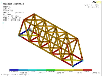
Figure 5: FE model with linear springs at support, maximum temperature of heating cycle.
Figure 5 shows the strain output of the bridge model for this loading con-dition. It is considerably easier to model the infrastructure behaviour with a uniform temperature gradient on all of its elements, but obviously this is a model discrepancy, since in the laboratory experiment the top of the bridge is much hotter than the bottom side, as seen in Figure4(a). Since the strain of the FE model is being sampled at the bottom side of the top bars the effect of the localised bending should be relatively small on the results.
3.3. Sensor location combinatorial analysis
This section presents a study of the influence of sensor location on the ca-pability of inferring the spring stiffness true value.
The modular Bayesian approach was applied to infer this parameter, based on all possible combinations of two out of eleven strain measurements available from the laboratory experiment. Only the first three modules of the algorithm are necessary for this combinatorial analysis. The resulting posterior distribu-tion is a Gaussian-shaped distribudistribu-tion whose moments (mean value and stan-dard deviation) estimate the stiffness value. Therefore of theC11
2 = 55 possible
combinations, the ones with minimum standard deviation σ[θ] and expected valueE[θ] closer to the spring stiffness real value were selected. This is pos-sible only because in this example the true value is known, and (%) can be determined.
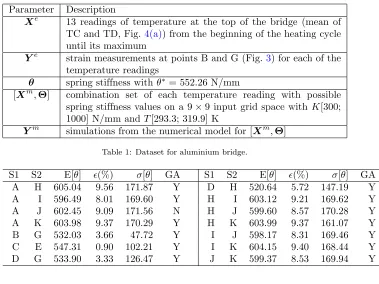
Parameter Description
Xe 13 readings of temperature at the top of the bridge (mean of TC and TD, Fig.4(a)) from the beginning of the heating cycle until its maximum
Ye strain measurements at points B and G (Fig.3) for each of the temperature readings
θ spring stiffness withθ∗= 552.26 N/mm
[Xm,Θ] combination set of each temperature reading with possible spring stiffness values on a 9×9 input grid space withK[300; 1000] N/mm andT[293.3; 319.9] K
Ym simulations from the numerical model for [Xm,Θ]
Table 1: Dataset for aluminium bridge.
S1 S2 E[θ] (%) σ[θ] GA S1 S2 E[θ] (%) σ[θ] GA
A H 605.04 9.56 171.87 Y D H 520.64 5.72 147.19 Y
A I 596.49 8.01 169.60 Y H I 603.12 9.21 169.62 Y
A J 602.45 9.09 171.56 N H J 599.60 8.57 170.28 Y
A K 603.98 9.37 170.29 Y H K 603.99 9.37 161.07 Y
B G 532.03 3.66 47.72 Y I J 598.17 8.31 169.46 Y
C E 547.31 0.90 102.21 Y I K 604.15 9.40 168.44 Y
D G 533.90 3.33 126.47 Y J K 599.37 8.53 169.94 Y
Table 2: Results of inference of the spring stiffness for different measurement combinations and≤10%.
S1 S2 E[θ] (%) σ[θ] GA S1 S2 E[θ] (%) σ[θ] GA
A C 430.84 21.99 58.79 N D F 433.96 21.42 65.98 Y
A F 444.54 19.51 68.20 N F G 640.50 15.98 67.50 Y
A G 687.24 24.44 47.97 N F I 439.67 20.39 65.44 Y
B D 394.75 28.52 68.56 Y G H 681.50 23.40 52.91 Y
B G 532.03 3.66 47.72 Y G I 684.32 23.91 50.80 Y
C G 608.89 10.25 58.89 Y G J 676.23 22.45 55.87 Y
C I 437.85 20.72 56.95 Y
Table 3: Results of inference of the spring stiffness for different measurement combinations andσ≤70 N/mm
respectively. The results show that:
• the combination of responses measured at point B and G provide the lowest error and variance on the inference of the spring stiffness;
present on Table 3), or the genetic algorithm optimisations do not con-verge (see the N on the GA column of Table 3). This indicates that measurements near model singularities such as supports tend to present poor identifiability;
• in general combining one measurement from the bridge bottom with one of the middle or top gives the lowest error and variances, which indicates that combining locations with a different loading range enhances identifiability.
To further support this interpretation, a comparison between an identifiability metric applied by Arendt [22] in his simulation, against our example shall be carried out in the following section.
3.4. Model calibration results and discussion
Considering the above results, the FE model was calibrated against the laboratory scale aluminium bridge. The design variable, response outputs and structural parameter are similar to what was presented for the combinatorial analysis in Table 1. The polynomial regression functions are set asH(•) = 1 and the prior of θ as a uniform probability density function (PDF). For this example the computational effort took 16.50 s on an Intel i7 quadcore 2.2 GHz, 6 GB of RAM and an SSD drive.
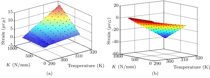
A mrGp of the model is presented in Figs. 6(a)and6(b), for the response surface of the strain at locations B and G. Hyperparameters are shown in Ap-pendix B. Notice how the uncertainty shrinks and increases relatively to the distance to the input dataset, to account for the uncertainty of the numerical model.
K(N/mm) Temperature (K)
Strain
(
µε
B
)
290 300
310 320
0 500 1000-5
0 5 10 15
(a)
K(N/mm) Temperature (K)
Strain
(
µε
G
)
290 300 310 320 0
500 1000 -60 -40 -20 0 20
(b)
Figure 6: 95 % prediction interval of the posterior multiple response Gaussian process - 40×40 grid with 9×9 grid input set (black dots) of strain at B6(a)and G6(b).
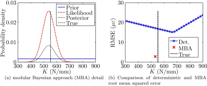
to a stiffness value of K= 661.5 N/mm with an error of 15.16µε. This error is more than five times larger than that of MBA (i.e. 2.82µε). Furthermore as seen in Figure7(b), the stiffness value resulting from MBA, 532.03 N/mm, is closer to the real value of stiffness given by the supplier 552.26 N/mm compared to the stiffness identified using the deterministic model identification. These results demonstrate the superior performance of MBA not only in terms of identifiability but also in the ability to predict structural responses. Despite the fact that the responses used for identification have the same characteristic nature (i.e. strain) the mean value and the variance closely approximate the real stiffness value. It is expected that if other responses such as displacements were given as input this uncertainty would be further improved.
K (N/mm)
Probabilit
y
densit
y
300 400 500 600 700 800 900 0
0.01 0.02 0.03
Prior Likelihood Posterior True
(a) modular Bayesian approach (MBA) detail
K (N/mm)
RMSE
(
µε
)
300 400 500 600 700 800 900 0
10 20 30
Det. MBA True
(b) Comparison of deterministic and MBA by root mean squared error
Figure 7: Inference of the stiffness of linear springs at aluminium bridge end, against reference value (vertical dashed line).
In comparison to the hierarchical Bayesian framework from Behmanesh [12] which had an estimation of model parameters with modelling errors at almost 20 % deviation from the true values (see Table 3 for clarification), our estimate deviated only by 3.66 %.
Also to further justify that the improvement on identifiability was achieved, mainly due to the sensor position and not the nature of the measured responses, a comparison between Arendt’s metric in his simulated example and our analysis was applied here. Essentially an improvement of identifiability by using multiple responses should be quantifiable through the posterior standard deviation of the model parameter that is being calibrated, following the formula (σSR
i,j,min−
σMR
i,j,post)/σi,j,SRmin where σij,SRmin = min(σi,post, σj,post) is the minimum posterior
standard deviation of the calibrated parameter with individual responses and σMR
i,j,post is the posterior standard deviation with multiple responses. In our case
an improvement of 10.1 % was observed which is similar to that of 14 % obtained by Arendt (see Table 3 of [22]), on his simply supported beam for responses with similar nature.
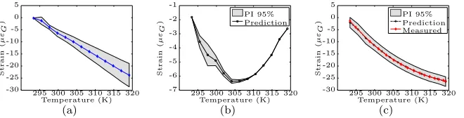
predic-tions for strain B and G are shown in Figure 8 and 9, respectively. Notice how the strain at B is positive for the model while negative in the experiment, and how the considerable discrepancy was predicted accurately on Figure8(b). The solid lines with diamond markers represent the measured response, which is within the uncertainty region. Since this region accounts for: uncertainty of the spring stiffness; model discrepancy; noise and the fact that the model response is known only at a set of discrete points (code uncertainty), the true undisturbed process should also fall within that limit with a 95 % accuracy.
Temperature (K) Strain ( µε B )
295 300 305 310 315 320 -1 0 1 2 3 4 5 6 7 8 9 (a) Temperature (K) Strain ( µε B )
295 300 305 310 315 320 -22 -20 -18 -16 -14 -12 -10 -8 -6 -4 -2 PI 95% Prediction (b) Temperature (K) Strain ( µε B )
295 300 305 310 315 320 -18 -16 -14 -12 -10 -8 -6 -4 -2 0 PI 95% Prediction Measured (c)
Figure 8: Strain at position B - Prediction interval 95 % confidence for numerical model8(a), discrepancy function8(b)and experimental response8(c).
Temperature (K) Strain ( µε G )
295 300 305 310 315 320 -30 -25 -20 -15 -10 -5 0 5 (a) Temperature (K) Strain ( µε G )
295 300 305 310 315 320 -7 -6 -5 -4 -3 -2 -1 PI 95% Prediction (b) Temperature (K) Strain ( µε G )
295 300 305 310 315 320 -30 -25 -20 -15 -10 -5 0 5 PI 95% Prediction Measured (c)
Figure 9: Strain at G aluminium bridge - Prediction interval 95 % confidence for numerical model9(a), discrepancy function9(b)and experimental response9(c).
4. Conclusions
This work applies a modular Bayesian approach on a structural identification framework. A combinatorial analysis to determine the best choice of a set of available sensors which maximises the identifiability of the problem was also per-formed. Afterwards, with these measurements a simplified model was calibrated against a reduced scale aluminium bridge experiment.
Based on the results the following conclusions can be inferred:
• It is possible to infer a fixed structural parameter with only two mea-surements of a single characteristic nature, even in the presence of high discrepancies as shown by the comparative study. This could be fur-ther improved by adding additional responses (three, four) with a more diversified nature (acceleration, displacement, etc.);
• Identifiability is influenced by the dependency of calibration parameters on measured responses. This is shown by measurements near singularities, such as supports of the bridge, which present poor identifiability relatively to measurements at the middle of the bridge. This is so because the dependency of the spring on the strain is smaller near supports;
• Temperature variations can be used to perform structural identification and establish uncertainty response baselines;
The methodology can also be expanded to consider multiple parameters, which is a common scenario on civil infrastructures [26,27,13].
Only two responses with the same nature have been used, which highlights the relevance of sensor placement. It could be relevant to compare the results of this work with an optimal measurement system design methodology, such as described in [31].
Appendix A. Emulation of numerical models with a Gaussian process
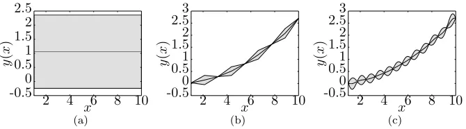
Since a numerical model is typically deterministic in nature and can take hours to compute it is useful to replace it with a probabilistic surrogate model. This current practice is known as metamodelling, or emulation [32]. Examples of this practice in SHM can be found on [27,26]. Also, applying a metamodel establishes a comprehensive framework for uncertainty analysis which eases the Bayesian inference process.
x
y
(
x
)
2 4 6 8 10
-0.5 0 0.5 1 1.5 2 2.5
(a)
x
y
(
x
)
2 4 6 8 10
-0.50 0.51 1.52 2.53
(b)
x
y
(
x
)
2 4 6 8 10
-0.50 0.51 1.52 2.53
(c)
Figure A.10: Prediction interval (grey cloud) and mean function (black line). As more data is being given (from10(a)to10(c)) the Gp model interpolates perfectly the input dataset.
point the mean function should be present and there should be no uncertainty; otherwise the mrGp should reflect a plausible interpolation or extrapolation of the available data, see Fig.A.10.
It is conventioned that in order to approximate the response surface, a dataset of [X,Y] with dimensions [N×d, N×q] shall be given as input. Dimen-sionsdand qrepresent the number of input design variables [x1x2. . .xd] and responses [y1y2. . .yq], whileN is the number of combinations of the whole in-put spaceXand associatedY. The prior mean function of the mrGp is assumed to belong to a hierarchical structure of linear functions, that in a generalised form can be written as M(X) = H(X)β, with matrix H(X) containing N polynomial linear functionsfj−1(x) : j = 1, . . . , p+ 1 of degree p(selected by
the user) and matrix of regression coefficientsβ, for each of the terms contained in matrixH(X) and each of theqfitted responsesY.
A typical choice for the prior covariance function which shall also be em-ployed here is the Gaussian form [34]
r(x, x0) = σ2
mexp
n
−Pd
i=1ωi(xi−x0i)2
o
(A.1)
whereσm2 is the variance of the response andωii= 1, . . . , dare called roughness parameters or length scales ranges [35] and they represent how roughly the response changes from each training data point to the next.
As proposed by Conti et al.[36] this structure can be generalised to an entire dataset by combining a spatial correlation function and a covariance between responses with the Kronecker product as
R(X,X0) =Σ⊗Γ(X,X0) (A.2)
withq×qcovariance matrixΣand aN×N correlation matrixΓthat contains the squared exponential function of equationA.1for all the (X,X’) inputs.
After having supplied a certain amount of data [X,Y] to the mrGp (assumed a non-informative prior forβ and givenωand Σ) the posterior distribution of the response atx0 is given by
y(x0)|Σ,ω,Y ∼ N(m∗(xo),Σ⊗γ∗(xo,xo)) (A.3)
with
m∗(xo) = h(x0) ˆβ+γ(x0)TΓ−1(Y −Hβˆ) (A.4)
γ∗(xo,xo) = γ(xo,xo)−γ(xo)TΓ−1γ(xo) + (A.5) [h(x0)T −HTΓ−1γ(x0)]T[HTΓ−1H]−1[h(x0)T −HTΓ−1γ(x0)],
γ(x0)T = [γ(x0,x1), . . . , γ(x0,xN)] as detailed in [37] andβis given by solving
HTR−1Hβˆ =HTR−1Y, which corresponds to the linear regression solution of the best linear unbiased predictor.
Fig.A.10). Hence the parameters that characterise the mrGp behaviour (hy-perparameters) and that have to be estimated areω,βandΣ. This is typically done by using maximum likelihood estimates (MLE), mainly for computational reasons.
Appendix B. Gaussian process hyperparameters
The following data represents estimates of parameters, that fully characterise the Gaussian processes, approximated on the modular Bayesian approach. They are named here as hyperparameters φ and comprise: a matrix of regression coefficientsβ, a variance matrixΣ, a noise variance matrixΛand the roughness parametersω. The numerical model mrGp has hyperparameters
ˆ
ωT ,K= [2.0 1.4] ˆ
βSB,SG= [−0.105 0.121] ˆ
Σ=
3.0645 8.4687 8.4687 25.3702
and the discrepancy function mrGp has hyperparameters
ˆ
ωT = 6.87 ˆ
βSB,SG= [−3.766 −0.242] Σˆ =
22.90 1.07 1.07 2.75
ˆ
Λ=
0.27 0.03 0.03 0.59
Acknowledgements
This work was supported by the Engineering and Physical Sciences Research Council (EPSRC) reference number EP/N509796.
Special thanks for the theoretical formulation review is referred to Sergio Jesus and technical support in the aluminium bridge case-study to Zong Tan, Arnett Taylor, Neil Gillespie and Colin Banks.
References
[1] Jesus AH, Dimitrovov´a Z, Silva MA. A statistical analysis of the dynamic response of a railway viaduct. Engineering Structures 2014;71. doi:10. 1016/j.engstruct.2014.04.012.
[2] Goulet JA, Smith IF. Structural identification with systematic errors and unknown uncertainty dependencies. Computers & Structures 2013;128. doi:10.1016/j.compstruc.2013.07.009.
[3] Erdogan YS, Gul M, Catbas FN, Bakir PG. Investigation of Uncer-tainty Changes in Model Outputs for Finite-Element Model Updating Us-ing Structural Health MonitorUs-ing Data. Journal of Structural EngineerUs-ing 2014;140(11). doi:10.1061/(ASCE)ST.1943-541X.0001002.
[5] Li PJ, Xu DW, Zhang J. Probability-Based Structural Health Monitoring Through Markov Chain Monte Carlo Sampling. International Journal of Structural Stability and Dynamics 2015;doi:10.1142/S021945541550039X. [6] Lam HF, Yang J, Au SK. Bayesian model updating of a coupled-slab system using field test data utilizing an enhanced Markov chain Monte Carlo simulation algorithm. Engineering Structures 2015;102. doi:10.1016/ j.engstruct.2015.08.005.
[7] Simoen E, Roeck GD, Lombaert G. Dealing with uncertainty in model updating for damage assessment: A review. Mechanical Systems and Signal Processing 2015;56–57(0). doi:10.1016/j.ymssp.2014.11.001.
[8] Beck J, Au SK. Bayesian Updating of Structural Models and Reliability using Markov Chain Monte Carlo Simulation. Journal of Engineering Me-chanics 2002;128(4). doi:10.1061/(ASCE)0733-9399(2002)128:4(380).
[9] Beck J, Katafygiotis L. Updating Models and Their Uncertainties. I: Bayesian Statistical Framework. Journal of Engineering Mechanics 1998;124(4). doi:10.1061/(ASCE)0733-9399(1998)124:4(455).
[10] Vanik MW, Beck JL, Au SK. Bayesian Probabilistic Approach to Structural Health Monitoring. Journal of Engineering Mechanics 2000;126(7). doi:10. 1061/(ASCE)0733-9399(2000)126:7(738).
[11] Cheung S, Beck J. Bayesian Model Updating Using Hybrid Monte Carlo Simulation with Application to Structural Dynamic Models with Many Uncertain Parameters. Journal of Engineering Mechanics 2009;135(4). doi:10.1061/(ASCE)0733-9399(2009)135:4(243).
[12] Behmanesh I, Moaveni B, Lombaert G, Papadimitriou C. Hierarchical Bayesian model updating for structural identification. Mechanical Systems and Signal Processing 2015;64-65. doi:10.1016/j.ymssp.2015.03.026. [13] Matos JC, Cruz PJ, Valente IB, Neves LC, Moreira VN. An innovative
framework for probabilistic-based structural assessment with an application to existing reinforced concrete structures. Engineering Structures 2016;111. doi:10.1016/j.engstruct.2015.12.040.
[14] McFarland J, Mahadevan S. Multivariate significance testing and model calibration under uncertainty. Computer Methods in Applied Mechanics and Engineering 2008;197(29-32). doi:10.1016/j.cma.2007.05.030.
[15] Higdon D, Gattiker J, Williams B, Rightley M. Computer Model Calibra-tion Using High-Dimensional Output. Journal of the American Statistical Association 2008;103(482). doi:10.1198/016214507000000888.
[17] Kuok SC, Yuen KV. Structural health monitoring of Canton Tower using Bayesian framework. SMART STRUCTURES AND SYSTEMS OCT-NOV 2012;10(4-5).
[18] Kennedy MC, O’Hagan A. Bayesian calibration of computer models. Jour-nal of the Royal Statistical Society: Series B (Statistical Methodology) 2001;63(3). doi:10.1111/1467-9868.00294.
[19] Brynjarsd´ottir J, O’Hagan A. Learning about physical parameters: The importance of model discrepancy. Inverse Problems 2014;30(11). doi:10. 1088/0266-5611/30/11/114007.
[20] Arendt PD, Apley DW, Chen W. Quantification of Model Uncertainty: Calibration, Model Discrepancy, and Identifiability. Journal of Mechanical Design 2012;134(10). doi:10.1115/1.4007390.
[21] Yuen KV. Bayesian Methods for Structural Dynamics and Civil Engineer-ing. In: Bayesian Methods for Structural Dynamics and Civil EngineerEngineer-ing. John Wiley & Sons, Ltd. ISBN 978-0-470-82456-6; 2010,.
[22] Arendt PD, Apley DW, Chen W, Lamb D, Gorsich D. Improving Identi-fiability in Model Calibration Using Multiple Responses. Journal of Me-chanical Design 2012;134(10). doi:10.1115/1.4007573.
[23] Laory I, Westgate RJ, Brownjohn JMW, Smith IFC. Temperature Varia-tions as Loads Cases for Structural Identification. In: Proceeding of the of 6th International Conference on Structural Health Monitoring of Intelligent Infrastructure (SHMII), Hong-Kong, 2013. Hong Kong; 2013,.
[24] Laory I, Trinh TN, Smith IF, Brownjohn JM. Methodologies for predicting natural frequency variation of a suspension bridge. Engineering Structures 2014;80. doi:10.1016/j.engstruct.2014.09.001.
[25] Yarnold MT, Moon FL. Temperature-based structural health monitoring baseline for long-span bridges. Engineering Structures 2015;86(0). doi:10. 1016/j.engstruct.2014.12.042.
[26] Spiridonakos M, Chatzi E. Metamodeling of dynamic nonlinear structural systems through polynomial chaos NARX models. Computers & Structures 2015;157. doi:10.1016/j.compstruc.2015.05.002.
[27] Wan HP, Ren WX. Parameter Selection in Finite-Element-Model Updat-ing by Global Sensitivity Analysis UsUpdat-ing Gaussian Process Metamodel.
JOURNAL OF STRUCTURAL ENGINEERING 2015;141(6). doi:10.
1061/(ASCE)ST.1943-541X.0001108.
[29] Kennedy MC, O’Hagan A. Supplementary details on Bayesian Calibration of Computer Models. Tech. Rep.; 2001.
[30] Swanson Analysis Systems IP I. ANSYS, Inc. Documentation for Release 15.0. 2013.
[31] Arendt PD, Apley DW, Chen W. A preposterior analysis to predict iden-tifiability in the experimental calibration of computer models. IIE Trans-actions 2016;48(1). doi:10.1080/0740817X.2015.1064554.
[32] Lophaven SN, Nielsen HB, Søndergaard J. DACE - A MATLAB Kriging Toolbox. 2002.
[33] O’Hagan A. Bayesian analysis of computer code outputs: A tutorial. Reli-ability Engineering & System Safety 2006;91(10-11). doi:10.1016/j.ress. 2005.11.025.
[34] Rasmussen CE, Williams CKI. Gaussian Processes for Machine Learn-ing. Adaptive computation and machine learning; Cambridge, Mass: MIT Press; 2006. ISBN 978-0-262-18253-9.
[35] Cressie NAC. Statistics for Spatial Data. Wiley series in probability and mathematical statistics; reviewed ed.; New York: Wiley; 1993. ISBN 978-0-471-00255-0.
[36] Conti S, O’Hagan A. Bayesian emulation of complex multi-output and dynamic computer models. Journal of Statistical Planning and Inference 2010;140(3). doi:10.1016/j.jspi.2009.08.006.
![Figure 1: Flowchart of the modular Bayesian algorithm, source [20].](https://thumb-us.123doks.com/thumbv2/123dok_us/1002770.1600113/4.612.154.469.406.631/figure-flowchart-modular-bayesian-algorithm-source.webp)