Single– and Multiple–Access Point Indoor
Localization for Millimeter Wave Networks
Joan Palacios, Guillermo Bielsa, Paolo Casari, Joerg Widmer
Abstract—Millimeter wave (mmWave) location systems not only provide accurate positioning for location-based services, but can also help optimize network operations, for example through location-driven beam steering and access point association. In this paper, we design and evaluate localization schemes that exploit the characteristics of mmWave communication systems. We propose two range-free algorithms belonging to the broad classes of triangulation and angle difference-of-arrival. The schemes work both with multiple anchors and with as few as a single anchor, under the only assumption that the floor plan and the positions of the mmWave access points are known. Moreover, they are designed to be lightweight, so that even computationally-constrained devices can run them. We evaluate our proposed algorithms against two benchmark approaches based on fingerprinting and angles of arrival, respectively. Our results, obtained both by means of simulations and through measurements involving commercial 60-GHz mmWave devices, show that sub-meter accuracy is achieved in most of the cases, even in the presence of only a single access point. The availability of multiple access points substantially improves the localization accuracy, especially for large indoor spaces.
Index Terms—Millimeter wave; localization; simulation; ray tracing; measurements; commercial 60 GHz hardware
I. INTRODUCTION
Millimeter-wave (mmWave) communications in the 30 to 300 GHz range are a disruptive technology for future high-rate wireless communications [2]–[4]. mmWaves are characterized by crisp reflections carrying significant power with little energy scattering around the direction predicted by the law of reflection [5], [6], and a predominance of the line-of-sight (LoS) component over reflected components in the absence of blockage [7]. These channel effects have been studied in great detail, e.g., in [6], [8], and the above characteristics imply a quasi-optical propagation behavior, which enables indoor localization methods based on geometrical propagation assumptions [9].
Indoor localization is considered an enabling technology for a range of applications [10], including people and asset
track-Manuscript received March 28, 2018; revised July 27, 2018 and October 16, 2018; accepted February 05, 2019. Date of publication XXX XX, XXX; date of current version XXX XX, XXX. This work has been supported in part by the ERC project SEARCHLIGHT (grant no. 617721), the Ramon y Cajal grant RYC-2012-10788, the Madrid Regional Government through the TIGRE5-CM program (S2013/ICE-2919) and the Spanish Ministry of Science, Innovation and Universities the DiscoEdge grant (TIN2017-88749-R). The associate editor coordinating the review of this paper and approving it for publication was P. Salvo Rossi.
A preliminary version of this work has been presented at the IEEE SECON 2016 conference [1].
All authors (e-mail: [email protected]) are with the IMDEA Networks Institute, 28918 Madrid, Spain. Joan Palacios and Guillermo Bielsa are also with University Carlos III of Madrid, 28918 Madrid, Spain.
Color versions of one or more of the figures in this paper are available online at http://ieeexplore.ieee.org.
Digital Object Identifier xx.xxxx/TWC.xxxx.xxxxxxx
ing, large-scale virtual reality, next-generation RFID tags [11], assisted living [12], tracking of patients in protected areas, as well as other functions related to social proximity and environment-dependent customization of mobile devices [13]. This makes it a hot topic for current theoretical and practical research, as proven by the broad participation to yearly lo-calization competitions such as [14]. Recently, some indoor localization algorithms have achieved remarkable accuracy. For example, Chronos [15] achieves a median error of about 70 cm and 1 m in LoS and non-LOS (NLoS) environments, re-spectively, using multi-channel WiFi signals. The competition report in [16] also shows that a very good average accuracy is achieved by some approaches such as [17] (infrastructure-based, mixing angle and distance measurements) and [18] (infrastructure-free, based on fingerprinting in dense WiFi deployments). Other systems achieve sub-meter accuracy by integrating WiFi signal processing with inertial sensors [19], or by deploying ultra-wideband devices [20], [21].
Importantly, accurate localization and tracking can serve as a proxy for physical mmWave communication functions, such as beam training [22], handover and context switching. While the degree of accuracy required for indoor localization may vary widely depending on the specific application, we remark that no extreme accuracy is required to assist, for example, handover and beam training/tracking in mmWave networks. In fact, the typical beamwidth of current mmWave hardware ranges between 7 and 10 degrees or more [23]. Such apertures translate into a horizontal span between 60 and 90 cm at 5 meters from the access point (AP), or between 90 and 180 cm at 10 meters. In this context, sub-meter accuracy would be more than sufficient to help choose the right sector for link establishment, or to help detect sector changes as a client moves.
Still, several characteristics of mmWave links require to rethink the typical localization methods employed in indoor environments. For example, according to the Friis equation, due to the short wavelength the path loss can easily exhibit 30 to 40 dB higher attenuation compared to microwave signals over typical link distances. Moreover, in some bands the spectrum has further absorption peaks (e.g., at 60 GHz, due to oxygen absorption) [9], [24]. While this implies that a LoS propagation path is easily distinguishable from NLoS paths, it also limits the range of indoor mmWave communi-cations, which is often confined to a single room or a portion thereof [25]. For communications, these effects are typically compensated for via antenna arrays that permit to form narrow and very directional beams, implying that LoS and NLoS components can be discriminated in the angle domain.
energy constraints. This requires to achieve sufficient accuracy without complex signal processing through a low-overhead design. The localization process can be aided in part by the anchor APs, which can simplify the environment estimation by broadcasting constraints such as room boundaries (walls, ceiling height, etc.) as well as their own position. Besides this information, the localization algorithms should rely only on the information that is available locally on the device, i.e., provided by the device’s RF interface.
In this paper, we propose two localization schemes for mmWave systems that work solely based on the angle mea-surements implicitly provided by the beam training process of mmWave devices. One of the schemes uses these measure-ments for a form of triangulation, and the other one uses them to compute angle difference of arrival (ADoA) values. The two algorithms offer different tradeoffs between accuracy and environment awareness requirements. They are designed to work with as many APs as are available in the indoor mmWave network, and leverage indoor multipath propagation in order to improve the localization accuracy. In conditions of particularly low coverage, these characteristics make it possible to localize a node with only a single AP. Note that, even in case the PHY layer of the mmWave devices cannot be easily modified to directly make angle of arrival (AoA) information available, sector information of the highly directional antenna arrays is available at the MAC layer [26], making very it easy to pass such angle-related information to higher-layer protocols. Our algorithms assume to know the indoor area’s floor plan and the location of the mmWave APs. This is a common assumption for indoor localization [27]–[31] and can be realized by means of map-based services [32]. However, we do not require the knowledge of temporary obstructions, such as human bodies blocking mmWave propagation paths. As long as such obstructions do not lead to a very low number of visible paths for the client, the loss of a few propagation paths does not hamper the functionality of the algorithms. Additionally, spurious paths originating from temporary reflections are very likely to be filtered out by the validation or optimization steps of the algorithms. The feasibility and practicality of our schemes is demonstrated through both simulations and experiments with commercial mmWave systems operating in the 60 GHz band, in two different indoor scenarios.
This paper substantially extends several aspects of our previous work [1]. First, while [1] is concerned with single-anchor localization, this work focuses on realistic mmWave deployments with multiple APs and extends all localization algorithms to work with multiple anchors. In this sense, the algorithms in [1] are a special case of those presented in this paper. When designing these improved algorithms, we adhere to the initial design requirement that localization should be achieved using only angle information as provided by the mmWave hardware (e.g., through sector information) and that the algorithms should have limited computational complexity. Moreover, we present several additional simulation results both for multiple and for a single anchor AP. These simulations are complemented by two sets of experimental results obtained with commercial mmWave hardware, including a multi-AP deployment in a realistic office space.
The remainder of this paper is organized as follows. Sec-tion II surveys related work. SecSec-tion III describes the proposed algorithms. Section IV discusses simulation results and draws initial conclusions on the performance of the algorithms, and Section V presents an experimental campaign involving actual mmWave hardware, which characterizes the performance of our localization algorithms in real-world environments. Fi-nally, Section VI draws concluding remarks.
II. RELATEDWORK
We subdivide related work on localization into a general review of classical schemes (Section II-A) and more recent advances (Section II-B).
A. Classical localization schemes
Trilateration and multilateration are among the most com-mon range-based localization methods [33]. Ranging can be provided via the evaluation of the Time of Arrival (ToA) or of the received signal strength (RSS) [34], if a path loss model is available. However, range-based approaches may suffer from inaccurate ranging in typical scenarios. Triangulation [33] requires the knowledge of the distance between two anchor nodes and of the angles of departure from the anchors. Here, angle estimation errors negatively affect the accuracy, especially if the distance between the client and the anchors is large. Fingerprinting-based methods [33], [35] rely on the assumption that measurable radio fingerprints are distinct for a given location. While the definitions of fingerprint vary broadly depending on the scenario and radio technology [36], this method has the significant drawback that a very high measurement effort is required for fingerprint collection (the greater the desired accuracy, the more measurements must be collected). The mathematical analysis of the error performance of schemes based on TOA, TDoA, RSS, and AoA in an NLoS environment is provided in [37] via Cramer-Rao bound expressions, observing that the AoA distance error tends to increase faster than TDoA or RSS errors. The fusion of ToA and RSS measurements via an adaptive likelihood metric in WiFi scenarios is advocated in [38]. The proposed algorithm works with the empirical distribution of such measurements and is robust to non-Gaussian noise, achieving a median error of about 2 m.
The choice of range-based or range-free methods depends on the availability of a precise path loss model: in general, range-based methods achieve better accuracy, but require to accurately tune the parameters of the path loss model in a way that is environment-dependent, and can lead to large errors if such parameters are wrongly estimated or updated too infrequently. In these cases, angle-based methods are preferable.
B. Recent advances in indoor localization
shown to be accurate but sensitive to changes in orientation and antenna height. CUPID [40] is a range-based system that extracts the direct propagation path in multipath WiFi environ-ments and locates a user using multiple RSSI measureenviron-ments. Centaur [41] fuses acoustic and radio-frequency ranging using Bayesian inference to achieve better accuracy than with either system alone. SAIL [42] exploits a single AP for localization, and improves the accuracy of position estimates through dead reckoning enabled by a smartphone’s sensors. The system needs to estimate the gait of the user carrying the smartphone, and is sensitive to pose changes. iLocScan [43] harnesses the multipath propagation of WiFi signals in order to localize a signal source and roughly estimate the surrounding boundaries. The approach is demonstrated using a USRP implementation of the algorithm and the related antenna array signal process-ing. The common aspect of these works is that multi-antenna signal processing is used to improve the performance of the localization algorithms, even in scenarios where only a single AP is available.
Especially mmWave technology is amenable to high-accuracy indoor localization [44]. The shorter mmWave wave-length, compared to microwave frequencies in the sub-6 GHz range, makes it possible integrate larger antenna arrays in a smaller space, enabling MIMO approaches for localiza-tion. By leveraging a sparse representation of the MIMO channel matrix, a localization technique based on ML was designed in [45]. However, such techniques are computation-ally intensive, and efficient implementations usucomputation-ally require programmable hardware such as FPGAs. The performance of RSS-, TDoA- and AoA-based localization schemes in mmWave systems is compared via simulations in [46], as-suming the presence of several anchor nodes deployed over a circumference around the receiver. It is observed that the AoA approach achieves the smallest localization error because of the broad AoA spectrum diversity originating from the circular geometry. Under the assumption of no initial environment knowledge, JADE [47] localizes a client based solely on ADoA information, and maps the environment by leveraging the relationship between physical and virtual anchors, where virtual anchors correspond to the reflected paths of physical anchors. While the method obtains sub-meter localization accuracy in simulations, it requires several APs in order to achieve a realistic map of the environment. A single-anchor pseudo-lateration method is proposed in [48] that estimates the position of a client by measuring the distance from a physical anchor and from a corresponding virtual anchor. Like other range-based methods, pseudo-lateration requires environment-dependent calibration in order to achieve good results. mmWave has been combined with different technolo-gies to localize a client. In [49], the authors consider uplink mmWave and downlink visible light communications, where the lowest error obtained was about 6 cm. For mmWave localization, the authors rely on a single multi-antenna anchor, and exploit reflected paths.
While mmWave systems make it possible to discriminate signals in the angular domain, ultra-wideband (UWB) systems discriminate different propagation paths in time, and enable accurate localization via time-of-arrival (ToA)-based ranging
techniques. In [50] the authors review UWB ranging tech-niques together with the primary sources of TOA error (e.g., clock drift, and interference). Fundamental ToA bounds are described in both ideal and multipath environments. UWB can potentially enable concurrent ranging [21], which has the potential to reduce the ranging time by allowing overlapping transmissions.
By observing that deterministic multipath components typi-cally bear up to 90% of the UWB channel impulse response’s energy, the authors in [51] employ a single anchor node, extract ToA information from the AoA spectrum, and estimate the distance between the client and physical or virtual anchors via an ML approach. The knowledge of the floor plan is assumed in order to identify the location of virtual anchors. In [52], the TDoA between different multipath components is used to compute range estimates via an ML approach. Filtering such estimates through a Kalman filter yields a median localization error below 5 m in simulations.
Cooperative localization is also a promising paradigm that improves the localization accuracy at the cost of exchanging information among the network nodes [53]. In the iterative algorithm DILOC [54], the nodes exchange location estimates and derive their position as the convex combination of the co-ordinated of a proper set of neighboring nodes. The process is initialized bym+1anchors in anm-dimensional environment. DILAND [55] improves over DILOC by supporting noisy distance measurements and unstable communication links. In the network navigation framework [56], the nodes localize themselves using internal measurements (e.g., inertial sensors) and intra-node measurements (e.g., radio ranging). The paper presents theoretical results to establish how navigation infor-mation evolves in a cooperative network. In [57] and [58] the authors develop a framework to characterize the fundamental limits of localization accuracy for a single client and in a wideband cooperative localization scenario, respectively. In the latter, it is assumed that the nodes exchange whole waveforms, instead of summary information such as ToA or RSS.
Table I
NOTATION EMPLOYED IN THE PAPER
Name Meaning Name Meaning
p,n,pn
tx Point, normal vector, location of APn An Set of the virtual anchor locations
NAP Number of APs A¯n Partition of setAn∪ {pntx}
Pn
p(α) AoA spectrum for APnat pointp Anµ Set of virtual anchors mirrored up toµtimes for APn Nn
p Number of MPCs inPpn(α) Aµ Set defined as
SNAP
n=1 Anµ
M(n,p) 2×Nn
p matrix with MPCs inPpn(α) vmax Number of anchors used for validation in TV
˘
M(p) Concatenation of allM(n,P)matrices β Vector such that APβigenerates MPCiinM˘(p)
δm Angle differenceM˘(2p,m) −M˘
(p)
2,1 Dn Set of fingerprints for APn
Z Set of obstacles F Set of fingerprint measurement locations
α0 Reference angle T(n,p) NLoS feature matrix (lastNpn−1rows ofM(n,p))
∆α Error onα0(compass bias) σ AoA estimation error
feature a high density of APs in order to guarantee sufficient coverage. Still, the algorithms also work under sparse deploy-ment conditions, and even in the presence of only a single access point.
III. MILLIMETERWAVELOCALIZATIONSCHEMES
We now present the localization algorithms, which are designed such that the client can run them locally by mea-suring only angle of arrival information. Such information is inherently available in mmWave scenarios, which implement directional communications through phased arrays, and run beam training algorithms to identify the best steering direction for the array’s main lobe [59], even in dynamic scenarios [60], [61]. The algorithms presented in the following are represen-tative of two broad classes of approaches, those based on triangulation and those based on ADoA. Such classes have different advantages and disadvantages. The first algorithm, named Triangulate-Validate (TV), requires fewer anchors to localize a client successfully, but is sensitive to errors in the device orientation. The second one is based on ADoA information, and has the advantage that it is inherently immune to orientation biases, but requires a larger number of anchors than TV. These algorithms will be compared against two benchmark approaches from the literature: the first is based on fingerprinting (FP) [1], [36], which is lightweight for the client, but requires the setup of a fingerprint database, typically implying a very significant measurement collection effort; the second one is named CCAL and is based on the solution of ADoA localization as a convex quadratic problem [62]. All algorithms are designed to leverage the sparse AoA spectrum that results from the quasi-optical mmWave propagation, and can manage the multiple APs that are typically encountered in indoor mmWave deployments. However, even if the indoor space is illuminated by only a single AP (for example in case other APs are blocked by obstacles), the algorithms can leverage multipath propagation in order to localize a node using both LoS and NLoS paths.
We now present the required background and notation. The most important symbols and definitions are collected in Table I. With focus on an indoor scenario, we define a three-dimensional Cartesian coordinate system centered in one of the corners of the room. The system is described by the canonical vectors ex = (1,0,0), ey = (0,1,0) (oriented
orthogonally along the floor sides), andez = (0,0,1)(oriented
along the height of the room), such that any point q =
qxex+qyey+qzezcan be mapped to a triple(qx, qy, qz). The
room boundaries and any other permanent obstacles containing radio-reflective surfaces are grouped in the reflective objects setZ. Obstacles are modeled as three-dimensional polyhedra with flat polygonal faces, straight edges and sharp vertices. We treat each face as an oriented surface S, represented by its normal vector
n= (p2−p1)×(p3−p1)
k(p2−p1)×(p3−p1)k
, (1)
where p1, p2 and p3 are points of S, k · k denotes the
Euclidean norm, and × the cross-product. We assume that one or more mmWave APs 1, . . . , n, . . . , NAP are installed
in the room at the locations p1
tx, . . . ,pntx, . . . ,p
NAP
tx . These
APs act as reference nodes for localization purposes. We also assume that each node trying to localize itself is aware of the location of the APs and of the obstacles in Z. This is in line with our assumption that localization must be attained even by devices with limited computational power or hard energy constraints. The algorithms are designed to leverage the reflections of the AP signals off indoor boundaries in order to compute location estimates. For every AP n, the input to our algorithms is the AoA spectrum Ppn(α), which records
the distribution (over the azimuthal plane) of the amplitude of multipath components (MPCs) of the signal from AP n, as seen at a given location p. The AoA spectrum is a function of the azimuth α, measured relative to a reference angle α0. For each AP n, Ppn(α) is processed to yield a compact
representation of different MPCs atp. In particular, a peak in the reception pattern is identified with an MPC [63]. An MPC can be either a LoS or an NLoS path. We remark that, with respect to the classical triangulation and angle-difference-of-arrival localization algorithms, our schemes are unaware of the correspondence between the APs and the MPCs, and do not know a priori whether an MPC corresponds to a LoS or an NLoS propagation path. Enacting procedures to estimate this correspondence and localize a node is a distinctive feature of our algorithms. Such procedures have been designed to have low complexity, thus avoiding exhaustive search or maximum likelihood approaches in the design of both TV and ADoA. We collect the MPCs related to every AP n in a 2×Nn p
matrix M(n,p), where Nn
p is the number of detected MPCs
inPn
Figure 1. Example scenario, including the geometry of angle difference-of-arrival localization.
each MPC sorted in decreasing order; the second row contains the AoA of the MPC, relative to the referenceα0. In this way,
each columnM(:n,p,k )ofM(n,p)(where the colon notation :,k
denotes all elements of the corresponding dimension, and in this case it means all rows of columnk) can be seen as a vector in polar coordinates, departing from p, where M(1n,p,k ) and
M(2n,p,k ) are the amplitude and phase of the vector relative to α0, respectively. Finally, we defineM˘(p)as the2×P
NAP n=1N
n p
concatenation of all matrices M(n,P), re-sorted in order of decreasing MPC amplitude, and we callβthe 1×PNAP
n=1N
n p
vector whoseith elementβi indicates the index of the AP that
generates the ith MPC in M˘(p). For simplicity, we describe
the algorithms developed in this paper for the case of node localization on the azimuthal plane, but their extension to the 3D case is straightforward.
A. Virtual anchors
The signals emitted by a given AP located at pn
tx generate
an AoA spectrum Pn
p(α) at location p. Each MPC in this
spectrum can be modeled as emitted by a virtual anchor that would be the source of a LoS signal reaching p along the same AoA of the MPC. The position of the virtual anchor can be determined by mirroring the location of APnwith respect to the surfaces where its signal incurs a reflection. CallAn=
{an0,an1, . . .} the set containing the positions of the possible virtual anchors for AP n, and call A¯n ={An
0, A
n
1, A
n
2, . . .}
a partition of the setAn∪ {pn
tx}. We letAn0 =pntx, whereas
each setAni,i= 1,2, . . .contains the virtual anchors that have been mirroreditimes with respect to any surface of the objects in Z. Note that there is no limit to the number of times the AP can be mirrored. However, in practice the mmWave signal of the AP will fade quickly as it propagates and reflects off multiple surfaces: this is a substantially different aspect with respect to, e.g., UWB systems at lower frequencies, and allows us to truncateAn by considering a maximum reflection order
µ [63]. To this end, we defineAn µ=
Sµ
i=0A
n i.
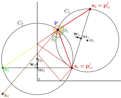
Fig. 1 shows an indoor scenario with two walls (thick gray lines) and two physical APs at locations p1tx and p2tx,
corresponding to anchorsa1anda2, respectively. Two virtual
anchors a3 and a4 correspond to a first- and a second-order
reflection, respectively, i.e.,a3∈A11 anda4∈A12.
B. The Triangulate-Validate (TV) algorithm
With this algorithm, a node at an unknown position p
estimates its position via a number of triangulation steps followed by a validation of the estimated locations. The algorithm assumes that the mmWave client has measured the AoA spectrum Pn
p(α) for each AP n, and has derived the
matrix M˘(p) and the vectorβ defined above. We recall that
the knowledge of the AP locations{pn
tx}
NAP
n=1, of the obstacle
set Z and of the reference angle α0 is also assumed. If
the association between the anchors in each set An and the
MPCs in M˘(p) were known, it would be possible to directly triangulate the position of p. However, we only assume to know the ID of the APs from which the MPCs in M˘(p)
originate, but not the physical or virtual anchor they are associated with. Hence, we have to estimate this association via the procedure explained in the following, which is designed to be significantly less complex than an ML approach [51].
With reference to the pseudo-code in Algorithm 1, we start by considering virtual anchors from all APs up to a reflection orderµ(line 3). While a high value ofµwould yield a richer virtual anchor set Aµ, a low value is more meaningful for
triangulation: in fact, reflections weaken the signal, and virtual anchors of higher order can be quite far from the receiver. In turn, this distance would translate into a large triangulation error, even for small angle errors in the AoA spectrum. In addition, a signal at mmWave frequencies is usually so weak after more than two reflections that it cannot be decoded. Hence, we set µ= 2in the following.
We start by considering M˘(:p,1) and M˘(:p,2) which, due to the sorting of M˘(p), correspond to the MPCs with highest amplitude. Before using them to triangulate a position, we need to transform these entries into vectors departing from the position of any anchor, expressed relative to the reference Cartesian coordinate system of the room. This yields two vectorsu1=−QM˘
(p)
:,1 andu2=−QM˘ (p)
:,2, whereQ is the
coordinate transformation (line 4). We now make an initial guess that the anchors from which u1 and u2 emanate are
two pointsa1, a2 ∈ Aµ. Given that there exist NAP APs in
the environment, each of which can be associated to multiple virtual anchors depending on the cardinality of set Z, we exploit the ID of the AP generating a virtual anchor in β
by imposing that ai ∈ Aβµi and aj ∈ A βj
µ (line 6). We then
triangulate a location by solving the following linear system in two unknowns t1≥0andt2≥0 (line 7):
ai+u1t1=aj+u2t2. (2)
to the floor map constraints (line 8),1 we validate the position by measuring how compatible the remaining MPCs are with the positions of other virtual anchors in Aµ. We assign a
weight wk > w` to all anchors of partition subsets Ank and
An
`, 0 ≤ ` < k ≤ µ, Ank, An` ⊂ Aµ, for all APs n. This
implements the consideration that the validations involving virtual anchors closer topshould be given greater importance. We now choosevmaxfurther MPCsM˘
(p)
:,m,3≤m≤vmax+2,
to be involved in the validation process. For each MPCm, we consider all virtual anchors inT =Aµr{ai,aj}and associate
a cost ck topk as follows:
ck=
vmax+2
X
m=3
min a∈T ∩Aβmµ
cos−1−um·
a−pk
ka−pkk
2
wω(a), (3)
where um = −QM˘
(p)
:,m and ω(a) =` if a ∈ An` for some
AP index n. We note that for a given MPC m, the argument of the sum is identically zero if there exists an anchora∈ T that lies exactly on the line leaving pk with direction M˘
(p) :,m,
whereas it increases if the minimum angle, centered in pk,
between any anchora∈ T andM˘(:p,m) increases. The squaring
operation penalizes large discrepancies (lines 9 to 15). After computing the argument of the minin (3), the anchor a that minimizes the argument is removed fromT (line 14).
The TV steps are repeated for all possible associations of
˘
M(:p,1)andM˘(:p,2)to the anchors in the setAµ, returning a total
of K estimates pk,k = 1, . . . , K, and their related costs ck
(line 6). Note that K ≤ |Aµ|(|Aµ| −1) since the algorithm
fails if a triangulated position is found to be outside the room, or if the ensemble of the AoA spectra received from all APs,
˘
M(p), contains fewer than 3 MPCs. The final estimate of p
returned by the TV algorithm is the one with the minimum associated cost (line 16). In lines 13 and 14, the function COST(pk,a,um), returns the argument of the min function
in (3). We remark that ifNAP= 1, Algorithm 1 falls back to
the triangulate-validate algorithm presented in [1].
C. The Angle Differences-of-Arrival (ADoA) algorithm
The TV algorithm requires the knowledge of the reference angle α0, or equivalently, of the coordinate transformation
matrix Q introduced in Section III-B. As this assumption cannot always be met, and the measurement of α0 (e.g., as
provided by a smartphone’s digital compass) may be affected by a significant error, we develop a second algorithm based on the Angle Differences-of-Arrival (ADoA) among MPCs. This algorithm is slightly more complex than TV, but is immune both to errors inα0 and to variations thereof across the room
area.
We start by defining the angles δ1 = ˘M (p) 2,2 −M˘
(p) 2,1 and
δ2 = ˘M (p) 2,3 −M˘
(p)
2,1. With reference to Fig. 1, that depicts
1The functionISVALIDcan be computed based on the winding number Wz(p), which equalsnif curvezrevolves aroundpntimes in the
counter-clockwise direction, and0if it does not enclosep. For indoor localization, we can assume without loss of generality that the curvesz∈ Zare traveled in the counter-clockwise direction by their parametric equationsz =z(t), 0≤t≤1, and that they have no loops. The logical functionISVALIDcan then be defined asISVALID(p,Z) =1 P
z∈ZWz(p) = 1, where1[p]is
Trueif predicatepis true, and the sum is identically 1 only if the client is inside the room, but outside any obstacle.
Algorithm 1: The Triangulate-Validate algorithm.
1 Function TRIANGVAL(Ppn(α)∀n,{pntx}
NAP
n=1,Z,α0,µ,
vmax,β)
2 Anµ←Sµ`=0DETERMINEANCHORS(`,pntx,Z)
3 Aµ←SNn=1APAnµ
4 Map M˘(p) to canonical base, computeu1,u2
5 k←0
6 foreachpair(ai,aj),ai∈ Aβµi,aj∈ A βj
µ ,ai6=aj do
7 pk ←point such thatai+u1t1=aj+u2t2
8 if ISVALID(pk,Z)then
9 T ← Aµr{ai,aj}
10 ck ←0
11 form= 3 tovmax+ 2 do
12 um← −QM˘
(p) :,m
13 ck ←ck+ mina∈T ∩Aβm
µ COST(pk,a,um)
14 T ←
T r{arg mina∈T ∩Aβm
µ COST(pk,a,um)}
15 k←k+ 1
16 returnpˆ =parg mink(ck)
a typical ADoA localization scenario, the ADoA algorithm is described as follows: given two pointsai andaj, find the
locus of the pointspsuch that the anglea\ipaj (wherepis the
corner), is constant and equal to the angle δ1 defined above.
This locus is a circumference, of which the segment aiaj is
a chord. The client is then located on this circumference. We assume the angle a\ipaj to be positive if ai follows aj in
the counterclockwise direction within the space of a semi-circumference and |a\ipaj| < π, where the | · | operator
represents the absolute value of the angle measure. In Fig. 1, consider the circumference C1. Given the angle a\1pa2, we
have a\1o1a2 = 2a\1pa2, where a\1o1a2 is the central angle
that stands on the same chord a1a2. Ifa\1pa2> π/2,a\1pa2
is concave, hence |a\1o1a2| > π. In this case, we wrap the
angle back into the interval [−π, π) via the operator W(·). The radiusr1 of C1 can be found as
r1=
ka1−a2k
2 sinW(a\1o1a2)
/2
. (4)
Finally, givenζ=r1cos W(a\1o1a2)/2
andu= (a−b)×
(0,0,1), the center of the circumferenceC1 is found as
o1=m1+ sgn
W(a\1o1a2)
ζu
kuk , (5)
wheresgn returns the angle sign, and m1 = (a1+a2)/2 is
the middle point ofa1a2. The vector
w1= o1−m1
sgn W(|a\1o1a2|)
(6)
points to the section of C1 defined by the chorda1a2 where
the constant angle requirement is satisfied. We now consider a second chord a1a3 and the circumference C2 as the locus
of the points q where the angle a\1qa3 =δ2. The radius r2
Algorithm 2:The Angle Difference-of-Arrival algorithm.
1 Function ADOA(P(α),{pntx}
NAP
n=1,Z,µ,vmax,β)
2 Aaµ←Sµ`=0DETERMINEANCHORS(`,pa
tx,Z)
3 Aµ←S NAP n=1 Anµ
4 Map M˘(p)to canonical base, compute δ1,δ2
5 `←0
6 foreach triple
(ai,aj,ak),a∈Aβµi,aj∈ A βj
µ ,ak∈ Aβµk,i6=j6=k do
7 C1← DETERMINECIRC(i,j,δ1)
8 C2← DETERMINECIRC(i,k,δ2)
9 p`←DETERMINEINTERSEC(C1, C2)r{pntx}
NAP n=1
10 if ISVALID(pk,Z) then
11 T ← Aµr{ai,aj,ak}
12 c`←0
13 form= 4to vmax+ 3do
14 c`←
c`+ mina∈T ∩Aβm
µ COST(p`,a,ai, δm)
15 T ← T r
{arg mina∈T ∩Aβm
µ COST(p`,a,ai, δm)}
16 `←`+ 1
17 return pˆ=parg min`(c`)
above. The intersection pbetweenC1 andC2is considered a
feasible location estimate whenever it is located on the sections of C1 and C2 pointed to by the orientation vectors w1 and
w2. This means that, given the two chord centersm1andm2,
it must hold thatw1·(p−m1)>0 andw2·(p−m2)>0.
The pseudo-code of the procedure that provides an estimate
ˆ
p of the location of a node based on ADoA is given in Algorithm 2. The algorithm starts by determiningAµ,M˘(p),
δ1 and δ2 (lines 3 and 4). As with the Triangulate-Validate
algorithm, we are initially unable to map each detected MPC to its related anchor node. Therefore, the ADoA algorithm collects a set of eligible positions which are the result of the intersection between the circumferences determined by the angle differences δ1 and δ2 and the chords aiaj and ajak, ai,aj,ak ∈ Aµ. Lines 7 to 9 determine the center
and radius of C1 andC2 via (4) and (5), and compute their
intersection p` by checking that it is feasible based on the
orientation vectors w1 and w2 (see Eq. (6)). At this point,
as for the TV algorithm, we pick vmax additional anchors
m = 4, . . . ,vmax+ 3 from M˘(p) (line 13), and for each of
them we compute δm = ˘M
(p) 2,m −M˘
(p)
2,1. The contribution
of MPC m to the cost of location p` (lines 14 and 15)
then depends on how well an anchor among those in set T =Aµr{ai,aj,ak} approaches the angle difference δm.
This cost is defined as follows:
COST(p`,a,ai, δm) = |ap\kai| −δm
2
(7)
The ADoA procedure is repeated for different triples
(ai,aj,ak)∈ Aµ (line 6), and the position with the minimum
associated cost is returned as the node location estimate (line 17).
Algorithm 3: ADoA fingerprinting-based localization.
1 Function FINGERPRINT(P(α),Dn,β)
2 ComputeM(n,p), extractT(n,p) 3 foreach f ∈ F do
4 cf ←0
5 foreach 1≤n≤NAP do
6 P(n)←
CLOSESTPAIRS T(2n,p,: ),T (n,f) 2,: −T
(β1,f)
2,1
7 foreach pair(i, j)∈ P(n) do
8 cf ←
cf +MPCCOST T
(n,p) :,i ,T
(n,f) :,j −T
(β1,f)
2,1
9 returnpˆ ←arg minfcf
D. Benchmark: Localization based on ADoA fingerprinting (FP)
We now present a fingerprint-based localization algorithm. Unlike TV and ADoA, FP does not strictly require that pntx,
n= 1, . . . , NAPandZ are known to the node to be localized.
We assume that the area has been previously characterized by creating a database Dn of AoA spectra for all APs,
measured at a set of different locations F = {f1,f2, . . .}.
Given a spectrum Pn
p(α) related to AP n and measured at
locationp, the algorithm looks up the most similar spectrum inDn (according to some proximity measure) and returns its
corresponding location. In order to be fair to the TV and ADoA schemes, we assume we can identify the LoS path, and define the fingerprint ofPn
p(α)in terms of the ADoA of
any NLoS path, computed relative to AoA of the LoS path. This choice is based on the fact that the strongest MPC is typically the LoS path [7], [63], and that we wish to make the feature matching process resilient to position-dependent errors in the reference angleα0. Given the patternPpn(α)and
its MPC matrixM(n,p), callT(n,p) the NLoS feature matrix that collects the lastNpn−1rows ofM(n,p), whereNpn is the
number of rows ofM(n,p). From all elements ofT(n,p) 2,: , we
finally subtract the angle of the LoS pathM(2n,p,1), in order to create a vector of ADoA NLoS features, which is finally used as a fingerprint. Note that with this definition, fingerprints are also immune to a non-zero bias on the reference angleα0. In
the pseudo-code in Algorithm 3, the above step corresponds to line 2.
The AoA spectra received at any two different points typically have one LoS feature, and may have a different number of NLoS features. For each entry of Dn measured
at location f (line 3), we execute an adapted instance of the closest point algorithm [64] which returns the indices i and j of the NLoS features in T(n,p) and T(n,f), respectively,
whose angle differences are most similar. The similarity of the patterns atpandf is finally conveyed by the cost
cf =− NAP
X
n=1
X
∀(i,j)∈P(n)
T
(n,p) 2,i −(T
(n,f) 2,j −T
(β1,f)
2,1 )
, (8)
0 2 5 8 10 0
2 10 13 15
3.5 8.5
pA
tx pBtx
pD
tx
pC
tx
Figure 2. Simulation scenario.
lines 7 and 8 computes the inner term of the sum in (8). These steps are repeated separately for each AoA spectrum corresponding to each of the APs. Finally, the algorithm returns the estimated position pˆ as the the location of the entryf ∈ F that has minimum cost (line 9).
E. Benchmark: a Convex-Combination based AoA Localiza-tion (CCAL)
We now describe the Convex-Combination based AoA Localization (CCAL) scheme [62]. This algorithm works based only on AoA information and exploits the presence of virtual anchors, hence it constitutes a good benchmark for our localization algorithms. CCAL develops from the observation that, in the presence of noisy angle measurements, client localization can be casted as an optimization problem with a non-convex objective function. The authors then propose a linear approximation to the objective function that makes the localization problem amenable to be solved. The use of virtual anchors makes it possible to bound the area where the source can be located in the presence of angle errors.
F. Complexity of the algorithms
The TV algorithm loops twice over the set of anchors and once over the total combination of AoAs and anchors in the MPC set. Therefore its complexity is O(maxn|An|3·vmax),
where maxn|An| is the maximum number of physical and
virtual anchors associated to any AP. The ADoA algorithm loops three times over the number of anchors and once over the number of AoAs and anchors in the MPC set. Its complexity is O(maxn|An|4·v
max). FP cycles once over the measurements
data set, once over the APs, and once to find the closest pairs of MPCs, which leads to a complexity of O(|D| ·maxn|An|2).
Finally, CCAL needs to solve a convexified quadratic prob-lem with O(NAP2 ) variables and O(NAP2 ) constraints, for which there exists a polynomial-time interior point algorithm. CCAL’s complexity is thus O(NAP12).We remark that the algorithmic complexity of TV, ADoA and FP is perfectly acceptable in typical indoor mmWave deployments.
1 2 3 4
Nº of APs 10-1
100 101
Location error [m]
ADoA FP TV CCAL
Figure 3. Statistics of the localization error for all algorithms as a function of the number of APs,NAP. The solid boxes indicate the quartiles of the
error distribution, the dashed error bars convey the 10th and 90th percentiles.
σ= 2◦,∆α= 0.
IV. NUMERICAL RESULTS
A. Simulation setup and scenario
In this section, we evaluate the performance of the proposed localization algorithms by means of simulation. We proceed by first describing an indoor space representing the network area as the input to a ray tracer; this includes the location of the APs and of the client, as well as the location of all walls. Second, for each position of the client, we run the ray tracer to simulate indoor mmWave propagation, and thereby retrieve the AoA spectra. Third, we run the localization algorithms of Section III using these AoA spectra and evaluate the localization error with respect to the true position of the client. We remark that no change is required to the algorithms with respect to the description in Section III.
The ray tracer is the same as described in [65, Section VI-B], and deterministically reproduces all relevant mmWave propagation phenomena, including path loss, material- and frequency-dependent reflection losses, shadowing and block-age. The output of the ray tracer collects the rays that lead to an actual received power contribution at the receiver (or eigenrays). Such output is translated into the AoA spectrum Pn
p(α) measured by the receiver at its location p. The AoA
spectrum is derived for every transmitting AP n, and is the input to all localization algorithms.
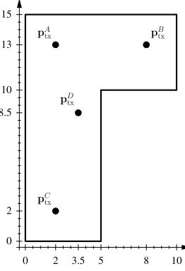
The simulation scenario consists of an L-shaped room, as depicted in Fig. 2. The vertical leg on the left is 5×15 m2, whereas the top-right section is 5×5 m2. We setα
0=π/2, i.e.,
angles are measured in a counterclockwise direction starting from the south-to-north direction. Up to four APs are located in the room at coordinatespAtx= (2,13)m,pBtx= (8,13)m,
pCtx = (2,2) m, and ptxD = (3.5,8.5) m. In the following, when we set NAP = 1, we activate only the AP at pAtx. For
NAP = 2we activate the APs at pBtx andpCtx; for NAP = 3
those at pAtx,pBtx, and pCtx. Finally, for NAP = 4, all of the
four APs in the room will be active.
For all algorithms, we truncate A to Aµ = S NAP n=1A
n µ by
considering only the virtual anchor nodes that correspond to up to µ = 1 reflections. We recall that different APs and virtual anchors become visible to the user as it moves. The fingerprinting algorithm has been trained through a reasonably dense set of measurements Dn for n = 1, . . . , N
1 2 3 4 Location error [m]
0 0.2 0.4 0.6 0.8 1
Cumulative Distribution Function
=1º =2º =5º
(a) TV
1 2 3 4
Location error [m] 0
0.2 0.4 0.6 0.8 1
Cumulative Distribution Function
=1º =2º =5º
(b) ADoA
1 2 3 4
Location error [m] 0
0.2 0.4 0.6 0.8 1
Cumulative Distribution Function
=1º =2º =5º
(c) FP
1 2 3 4
Location error [m] 0
0.2 0.4 0.6 0.8 1
Cumulative Distribution Function
=1º =2º =5º
(d) CCAL
Figure 4. CDF of the localization error for TV, ADoA and FP as a function of the standard deviation of the MPC angle estimation error,σ.NAP = 2,
∆α= 0.
includes a uniform matrix of 8×4 points in the vertical room section on the left, and 4×4 points over the top-right section. We simulate the fact that the measurement of the AoA spectrum by the node to be localized is not ideal, but rather may be affected by errors ∆α on the reference angle α0
as well as on the AoA estimates of the MPCs, e.g., as a consequence of small changes in the propagation environment, or due to imperfect beamforming of the phased antenna array at the receiver. This non-ideal behavior is modeled for a given position p by first estimating the true AoA spectrum, by extracting the MPC matrix M(n,p) for any AP n, and by
adding a different random Gaussian-distributed displacement of standard deviation σto the elements of M(2n,p,: ). To derive realistic MPC angle estimation errors, we synthesize beam patterns for a uniform linear antenna array with 8, 16 and 32 elements. For typical signal-to-noise ratios, these correspond to zero-mean Gaussian-distributed errors of standard deviation σ= 5◦,σ= 2◦, andσ= 1◦, respectively.
B. Simulation Results
We characterize the performance of the algorithms through the statistics of the localization error, as well as via the median location error experienced at different locations throughout the room. In our analysis, we explore the effect of different values
ofNAP,σand of the bias on the reference angleα0, denoted
as ∆αand called compass bias for short in the following. In Fig. 3 we show a box plot for the localization error incurred by ADoA, FP and TV for different values of NAP, for the
case of σ= 2◦ and∆α= 0.
We observe that even with one AP, TV, ADoA and FP achieve a sub-meter localization accuracy in at least 50% of the cases. However, since forNAP= 1the illumination of the
room is sub-optimal, the dispersion of the error is significant for both ADoA and FP, whereas 95% of TV’s errors are within less than 1.5 m. Conversely, CCAL does not perform well. While some positions experience small localization errors, these constitute a minor fraction of the cases, and the median error is about 8 m. The main reason behind this is that CCAL is not very robust to angle errors larger than those presented in [62], i.e., up to±0.1◦. IncreasingNAPimproves
the mmWave illumination across the room and some of the algorithms benefit from this. TV’s localization error decreases for increasing NAP, and levels off for NAP ≥ 3. Since
the statistics of FP’s localization error improve marginally for increasingNAP. CCAL’s performance improves forNAP= 2,
but then the error increases if additional APs are included. The reason is that, with an increasing number of APs, the set of virtual anchors grows, breaking the assumptions behind the linear approximation of the angles in [62]. We remark that the above results cannot be achieved by the TV, ADoA, and FP algorithms originally presented in [1], as they cannot leverage the presence of multiple APs.
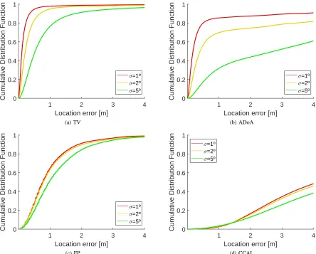
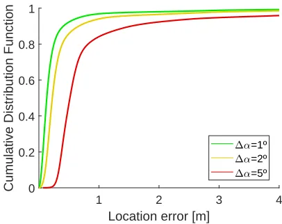
We now consider the effect of MPC estimation errors on the performance of the algorithms. Fig. 4 presents four graphs, one for each of the TV, ADoA, FP and CCAL algorithms. In each panel, we plot the cumulative distribution function (CDF) of the localization error, for σ = 1◦, σ = 2◦ and σ = 5◦. We
remark that the latter represents a very unfavorable case, with 97% of the angle estimation errors comprised in an interval of±15◦around the true AoA of each MPC. For this analysis, we set NAP = 2 (which is also the best case for CCAL)
and ∆α = 0. From panel 4a, we observe that while the performance of TV decreases for increasingσ, the localization error statistics remain very good even forσ= 5◦: in this case, the probability of achieving a sub-meter localization error is about 0.8, and decreases to 0.93 and 0.99 for σ = 2◦ and σ = 1◦, respectively. The situation is slightly different with ADoA (panel 4b), as an error of variance σ2 on the MPC angle estimation translates into an error of variance 2σ2 on angle differences. This adds to ADoA’s need to observe a higher number of MPCs than TV, and results in a higher maximum error. The probability of sub-meter accuracy for ADoA is 0.88 for σ = 1◦, but decreases to about 0.35 for σ = 5◦. The FP algorithm (panel 4c) behaves differently: depending on the value of σ, the probability of achieving a sub-meter localization accuracy ranges between 0.5 and 0.62. Specifically, for low values of σ, the limiting factor is the density of points in FP’s training data set; forσ= 5◦, instead, the effect of wrong MPC angle measurements dominates, and makes the AoA spectra measured by the client more similar to fingerprint database entries associated to farther positions. The results of CCAL (Fig. 4d) are aligned with those in Fig. 3, as the algorithm achieves sub-meter accuracy in less than 10% of the cases, and is characterized by a very high maximum error, above 4 m in at least 50% of the simulated estimates. Considering that FP requires to actually collect and maintain a training database, and given that FP’s performance is worse than TV’s and ADoA’s even forσ= 1◦, we conclude that FP is not a competitive algorithm for indoor mmWave localization. The same conclusion can be drawn for CCAL due to its unsatisfactory performance.
Finally, in Fig. 5 we evaluate the effect of a non-zero value of the compass bias∆αon the performance of TV for the case NAP= 3,σ= 2◦. We remark that ADoA and FP are immune
to non-zero values of ∆α by design. Compared to Fig. 4a, the average and maximum errors achieved by TV increase. While 98% of the estimated locations are within 1 m of the true client location for ∆α = 1◦, for higher values of ∆α we observe that the minimum error increases to about 30 cm, and the fraction of location estimates with sub-meter accuracy decreases to about 82%.
1 2 3 4
Location error [m]
0 0.2 0.4 0.6 0.8 1
Cumulative Distribution Function
=1º =2º =5º
Figure 5. CDF of the localization error for TV as a function of the client’s compass bias,∆α.NAP= 3,σ= 2◦.
In order to investigate the source of the errors observed for the TV, ADoA, FP, and CCAL localization methods in our simulation scenarios, we depict in Fig. 6 a heat map of the median localization error throughout the simulation area for NAP = 2 and∆α = 0◦. Dark-blue hues represent
near-zero error, whereas yellow hues represent high error. Fig. 6 reveals that TV achieves the lowest error throughout the map. A few areas of uncertainty exist for TV, mainly close to the walls. In these regions, the location of the client is estimated to be outside the boundaries of the area, therefore the validation step of the TV algorithm discards the estimate. For ADoA, we observe a generally very good performance, but high-error areas around both APs. These are the areas where the three strongest anchors and the client’s location tend to lie on the same circumference. As a result, the ADoA localization problem becomes ill-conditioned, and the localization error increases. The FP algorithm (Fig. 6c) also achieves a remarkably good error in this case. In some areas, this error increases significantly due to the similarity among arrival patterns throughout the room. Further results obtained with a four times-denser training set (not included due to lack of space) show that FP’s performance improves, but not substantially, leaving areas affected by significant errors close to the bottom and leftmost walls. CCAL’s error (Fig. 6d) shows that acceptable errors concentrate near the bottom-right and top-right corners of the L-shaped room: in these areas, the assumptions behind CCAL are verified and the linear approximation to its cost function is accurate. Otherwise, large errors occur as also noted above. These results confirm our preliminary conclusion that FP and CCAL are not preferred solutions for indoor mmWave localization.
While TV shows generally good performance under most conditions considered here and tends to outperform both ADoA and FP in a number of cases, it remains very sensitive to a biased reference angleα0, which instead does not affect
0 2 4 6 8 10 x-axis (m)
0 5 10 15
y-axis (m)
TV Error map
(a) TV
0 2 4 6 8 10 x-axis (m)
0 5 10 15
y-axis (m)
ADoA Error map
(b) ADoA
0 2 4 6 8 10 x-axis (m)
0 5 10 15
y-axis (m)
FP Error map
0 0.5 1 1.5 2 2.5 3 3.5 4 4.5 5
(c) FP
0 2 4 6 8 10 x-axis (m)
0 5 10 15
y-axis (m)
CCAL Error map
0 0.5 1 1.5 2 2.5 3 3.5 4 4.5 5
0 2 4 6 8 10 x-axis (m)
0 5 10 15
y-axis (m)
FP Error map
0 0.5 1 1.5 2 2.5 3 3.5 4 4.5 5
(d) CCAL
Figure 6. Median localization error maps for all methods,σ= 2◦,NAP= 2,∆α= 0.
0 2 4 6 8 10 x-axis (m)
0 5 10 15
y-axis (m)
TV Error map
(a)σ= 2◦,∆α= 0◦
0 2 4 6 8 10 x-axis (m)
0 5 10 15
y-axis (m)
TV Error map
(b)σ= 2◦,∆α= 5◦
0 2 4 6 8 10 x-axis (m)
0 5 10 15
y-axis (m)
TV Error map
(c)σ= 5◦,∆α= 0◦
0 2 4 6 8 10 x-axis (m)
0 5 10 15
y-axis (m)
TV Error map
0 0.5 1 1.5 2 2.5 3 3.5 4 4.5 5
(d)σ= 5◦,∆α= 5◦ Figure 7. Median localization error maps for TV, for different values ofσand∆α.NAP= 3.
significant reference angle bias ∆α= 5◦ leads to acceptable errors, mostly below 1 m (Fig. 7b). For σ = 5◦, instead, the superposition of inaccurate AoA estimates and a high
∆αimplies that the error remains generally high, with small regions of sub-meter errors, mainly close to the three APs.
V. EXPERIMENTAL RESULTS
We now perform experiments with actual mmWave hard-ware in realistic propagation scenarios, in order to validate the simulation results described in Section IV. We focus only on TV and ADoA for our experimental results, due to the worse performance shown by CCAL and FP. Furthermore, collecting and updating a training database in a fully operational and time-varying environment involves a significant effort and is very cumbersome for practical deployments.
We consider two scenarios: an empty room of size 6.3×8.9 m with a single AP installed (also considered in [1] and re-evaluated here to compare our new algorithms); and a more complex, fully functional L-shaped office area with typ-ical open-space furniture, including workstations and screens, as well as building elements such as columns and glass walls with metal frames. In the L-shaped room, we install up to 5 APs in order to achieve good coverage. The latter is
representative of dense mmWave AP deployments as are en-visioned in the literature to provide adequate indoor mmWave performance [24]. The empty room was chosen so that the LoS mmWave signal can be received clearly at all locations in the room, whereas the L-shaped room is representative of an actual working environment with signal blockage, such that the localization algorithms have to rely more heavily on both the real and virtual anchors they can observe at a given time.
A. Empty room with a single AP
0.1 0.2 0.3 0.4 0.5 0.6 0.7 0.8 0.9 1 −0.4
−0.2 0 0.2 0.4 0.6
Time [ms]
Amplitude [V]
1 2 3 4 5 . . . 32
32 frames
Figure 8. Dell D5000’s device discovery frames. Each frame corresponds to a different configuration of the station’s 2×8 phased antenna array [1], [66].
30
210 60
240
90 270
120
300
150
330
180 0
Sim Exp
Figure 9. AoA spectrum in the empty room at coordinates (1.85,5.75)m. (Adapted from [1].)
discovery frames are sent every 102.4 ms. For additional details, we refer the interested reader to [66].
For the receiver we use a 60-GHz VubIQ development sys-tem, connected to an Agilent MSO-X 3034 oscilloscope and equipped with a standard 25 dBi-gain horn antenna mounted on an Arduino-controlled rotating stage. The VubIQ reveals LoS paths as well as any MPC reflected off the boundaries of the room at any given position. We input the VubIQ’s down-converted, 1.8 GHz-bandwidth, analog modulated I/Q output signals directly into the oscilloscope, which digitizes and stores the traces for analysis. In this way, we collect the amplitude of each of the 32 discovery frames over the azimuthal plane. We control the rotating stage to take measure-ments at orientations spaced 3◦ apart. For every orientation, the receiver captures all 32 frames as in Fig. 8, where each frame is received with a different amplitude in each position, depending on the antenna patterns used by the D5000 for each frame and the mmWave signal propagation throughout the room. From these traces, an AoA spectrum is extracted by measuring the amplitude of the strongest frame. This replicates the behavior of a typical mmWave beam training handshake, where two devices would try several combinations of the beam pattern configurations available to them, until the best transmit and receive beam patterns are found. Fig. 9 shows one of the experimental patterns (in gray), measured at position
(1.85,5.75) m (see also Fig. 10 for a reference about the location). We observe that the LoS path between the D5000 and the VubIQ has an AoA of 215◦. Strong reflections are detected with AoAs of 125◦and 340◦, and a weaker reflection has an AoA of 30◦. For comparison, we also plot an AoA spectrum simulated via ray tracing (in black), which proves the very good agreement between ray tracing simulations and measurements.
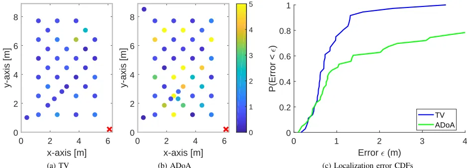
We carried out AoA spectrum measurements at a total of 44 points throughout the room. Figs. 10a and 10b show the localization performance of TV and ADoA, respectively, for all of the measurement points. The color of each circle conveys the accuracy of the position estimate: blue hues correspond to low error, whereas green and yellow hues correspond to increasingly higher errors. A red cross in the bottom-right
corner of the room represents the location of the D5000 docking station, i.e., the mmWave AP. The validity of each position estimate is checked against the room boundaries (this corresponds to the ISVALID(·) function in Algorithms 1 and 2). The 30 cm×30 cm area surrounding the location of the AP is also marked as an invalid location.
In general, TV achieves better localization performance than ADoA, with most estimated positions within 1 m of the true client location. The largest localization errors are primarily due to the large widths of some arrivals in the measured AoA spectra, which make it difficult to accurately estimate the corresponding AoA. Specifically, for the locations near the transmitter, this is the case for the LoS AoA. For TV, wrong AoA estimates result in wrong triangulated positions, which are found to be outside valid room boundaries. For this reason, TV is unable to localize the node at seven locations out of 44: two close to the AP, two concentrating around the measurement point at(3.8,2.5), and three at the opposite end of the room. As ADoA requires at least three MPCs in the AoA spectrum to work properly, the weakness of the received signal and the presence of mainly low-SNR second-order re-flections in some measurements throughout the room explains why ADoA incurs a large error at such locations. Fig. 10c summarizes the results by showing the cumulative distribution function (CDF) of the localization error, for the points for which a valid position can be estimated. We observe that both TV and ADoA achieve a sub-meter median error. While the probability to compute a very accurate location estimate is similar for both algorithms, overall TV has significantly higher location accuracy: its probability to obtain a sub-meter location error is about 0.8, against about 0.5 for ADoA.
B. L-shaped working area with multiple APs
0 2 4 6 8
y-axis [m]
0 2 4 6
x-axis [m] (a) TV
0 2 4 6 8
y-axis [m]
0 2 4 6
x-axis [m] (b) ADoA
0 1 2 3 4 5
0 1 2 3 4
Error (m) 0
0.2 0.4 0.6 0.8 1
P(Error <
)
TV ADoA
(c) Localization error CDFs
Figure 10. Map and CDF of the localization error of TV and ADoA in the empty room with a single AP.
AP5
AP2
RX client
Figure 11. Photo of the open space measurement setup of Fig. 12, showing the client, AP2 and AP5.
AP5
Figure 12. Multi-AP measurement setup in the L-shaped room area. Five different APs are deployed, each using one of three different antenna types (omnidirectional, 120◦-aperture and 80◦-aperture).
As the room is larger and contains different types of obstacles, a single AP cannot cover the whole area. We there-fore investigate scenarios including up to five APs deployed throughout the room. We remark that using D5000 docking stations would make it difficult to differentiate among the signals transmitted by each AP. We solve this issue by using the following five transmitters: one Pasternak VubIQ, two SiversIMA DC1005V/00 and two SiversIMA CO2201A. In order to be able to separate each platform’s signal at the receiver, we tune the local oscillator of each device to a different frequency within the 60 GHz band. Each transmitter is equipped with antennas of different beam widths, depending on the location of the transmitter, with the general objective of covering as much space as possible, so that the maximum number of transmitter signals can be seen and simultaneously sampled from every location in the room.
To emulate the user, we use the same Pasternak VubIQ receiver as before, equipped with a 7◦, 25 dBi-gain horn antenna. However, instead of connecting the VubIQ output to the oscilloscope, we use an Agilent EXA N9010A signal analyzer, capable of recording the mmWave signal and of differentiating between the different frequencies of the
trans-mitters. We take measurements at angular steps of 0.45◦, which covers the azimuthal plane with 800 measurements in total. We use pseudo omni-directional transmitters in order to speed up the collection of the measurements and capture all available paths of a given AP at the same time. As a general rule-of-thumb, we equipped APs located in open areas with an omni-directional antenna; where omni-directionality is not needed we employed wide-beam antennas (e.g., 80◦ -aperture horn antennas for APs near corners, and open wave-guide terminations translating into a 120◦antenna aperture for APs located near walls). After collecting the measurements for the different locations, we retrieve the AoA patterns for each AP by isolating the corresponding frequencies throughout all rotation steps. Different peaks in each pattern correspond to the LoS arrival (when available) and to one or more NLoS arrivals. Fig. 11 shows a view of the deployment.
0 2 4 6 8 10
Error (m)
0 0.2 0.4 0.6 0.8 1
CDF
NAP = 1
N
AP = 2
NAP = 3
N
AP = 5
(a) TV
0 2 4 6 8 10
Error (m)
0 0.2 0.4 0.6 0.8 1
CDF
NAP = 1
N
AP = 2
NAP = 3
N
AP = 5
(b) ADoA
Figure 13. CDF of the localization error for TV and ADoA for the multi-AP deployment in the L-shaped room, for different numbers of active APs.
transmitter in the lower east corner. We measured the AoA pattern from all visible APs at 66 different positions, with an average separation of 1.3 m between nearest measurement points. Note that the furniture constrained the measurements, which were taken around the work stations, in empty areas, and along the corridors. The opacity of glass to mmWaves and the resulting lack of coverage prevented us to do measurements in the offices and labs surrounding the open area.
We evaluate the performance of TV and ADoA in the above scenario for different numbers of active APs between 1 and 5. For the cases of 1 to 3 APs, we test the outcome of all possible choices of active and inactive APs, and select the combination that yields the best results. For example, for a single active AP, the best choice is AP 2 in Fig. 12, which provides the maximum area coverage compared to all other APs. For the case of two active APs, the best APs are AP 2 and AP 4, where the latter provides additional coverage especially around the top-left corner of the open area.
Fig. 13 shows the CDF of the localization error for the best combination of 1, 2, 3, and 5 active APs. As expected, when NAP= 1(only AP 2 is active), the localization error is
good in some cases, but still significant: sub-meter accuracy is achieved in roughly 30% of the estimates for TV and 5% of the cases for ADoA, and the maximum error of both algorithms is large as well. Increasing the number of APs improves the mmWave coverage throughout the room, so that the accuracy of both TV and ADoA increases. For example, sub-meter accuracy is achieved by TV in about 60% of the cases with 2 active APs, and up to 85% of the cases with 5 APs. ADoA’s performance increases similarly with additional active APs, up to a 70% probability of sub-meter accuracy with 5 active APs. This confirms that, in a realistic deployment, ADoA needs additional anchors (hence better mmWave coverage) in order to be able to compute the client location correctly.
In those locations where the localization outcome is in-accurate, the cause of the errors is typically traced back to insufficient mmWave illumination, as is the case in the
top left and rightmost sections of the room. In some cases, the validation step fails because localization errors make the predicted location exceed the room boundaries. Other possible sources of error are the alignment of anchors with the location of the users (which makes the triangulation problem ill-conditioned), or the case where the three strongest anchors and the client’s location lie on the same circumference (which makes the ADoA problem ill-conditioned).
VI. CONCLUSIONS
In this paper, we developed two localization algorithms tailored to the characteristics of mmWave propagation: one based on a Triangulate-Validate (TV) procedure, and one based on Angle Difference-of-Arrival (ADoA) information. We characterized the performance through measurements in-volving commercial 60-GHz mmWave hardware, both in an empty room and in a fully operational work environment that was in use during the measurements. Our results show that unless a large error affects AoA estimates, our algorithms achieve a very good localization performance. Specifically, they achieve sub-meter accuracy with high probability in the presence of sufficient mmWave illumination. An extensive set of simulations that compare TV and ADoA against an algorithm based on fingerprinting and an ADoA and virtual anchor-based algorithm from the literature show that TV is in general a better choice, especially when the orientation of the client can be accurately estimated. Conversely, the ADoA algorithm is immune to any compass bias, and is thus a better choice if the device orientation is affected by large errors.

![Figure 8.Dell D5000’s device discovery frames. Each frame corresponds to a differentconfiguration of the station’s 2×8 phased antenna array [1], [66].Figure 9](https://thumb-us.123doks.com/thumbv2/123dok_us/1108814.1612018/12.612.58.543.57.212/figure-discovery-frames-corresponds-differentconguration-station-antenna-figure.webp)