Disclaimer: The opinions, advice and information contained in this publication have not been provided at the request of any person but are offered by Australian Pork Limited (APL) solely for informational purposes. While APL has no reason to believe that the information contained in this publication is inaccurate, APL is unable to guarantee the accuracy of the information and, subject to
any terms implied by law which cannot be excluded, accepts no responsibility for loss suffered as a result of any party’s reliance on the accuracy or currency of the content of this publication. The information contained in this publication should not be relied upon for any purpose, including as a substitute for professional advice. Nothing within the publication constitutes an express or implied
warranty, or representation, with respect to the accuracy or currency of the publication, any future matter or as to the value of or demand for any good.
Quantifying Greenhouse Gas Emissions from
Australian Piggeries
Final Report
APL Project 2008/2232
November 2008
Department of Employment, Economic Development and Innovation
2 Table of Contents
1.1.1 Table of Tables ... 3
1.1.2 Table of Figures ... 3
2 Executive Summary ... 4
3 Introduction ... 7
4 Emission Measurement Techniques ... 8
4.1 Chamber Techniques ... 9
4.1.1 Flow-Through Steady State Chamber 9
4.1.2 Non-Flow-Through Non-Steady-State Chambers ...10
4.1.3 Flow-Through Non-Steady-State Chambers ...12
4.1.4 Application Contexts ...13
4.1.5 Strengths and Weaknesses...14
4.2 Mass Balance Techniques ...14
4.2.1 Closed or Mass Difference Systems ...15
4.2.2 Open or Integrated Horizontal Flux Systems ...16
4.2.3 Application Contexts for Mass Balance Techniques ...18
4.2.4 Strengths and Weaknesses of Mass Balance Techniques ...19
4.3 Backward Lagrangian Stochastic Techniques ...19
4.3.1 Robust Measurement ...21
4.3.2 Application Contexts for BLS Techniques...22
4.3.3 Strengths and Weaknesses of BLS Techniques ...22
4.4 Landscape Scale Micrometeorological Methods ...23
4.4.1 Eddy Covariance ...23
4.4.2 Eddy Accumulation ...24
4.4.3 Relaxed Eddy Accumulation...24
4.4.4 Flux Gradient Methods ...25
4.5 Online, Offline, Closed Path or Open Path Analysis?...27
4.6 Recommended Approach ...30
5 The Nitrous Oxide Emission Processes ...32
5.1 Nitrogen Transformations and Processes ...32
5.2 Nitrous Oxide Emissions ...34
5.2.1 Direct Emissions ...34
5.2.2 Indirect Emissions through Ammonia Volatilisation ...39
5.3 Data Regarding Manure and Effluent Application to Land ...41
5.3.1 Piggery Manures and Effluents Compared to Other Sources...42
5.3.2 Effect of Effluent Treatment Process ...47
5.3.3 The Influence of Application Technique and Combined Inorganic-N Fertiliser Applications on Nitrous Oxide Emissions ...48
5.3.4 Effluent and Spent Deep Litter Storage Emissions ...48
5.3.5 Diet ...50
5.3.6 Emissions from Housing ...50
5.4 Process Algorithms ...51
6 Conclusions and Recommendations ...54
3
1.1.1 Table of Tables
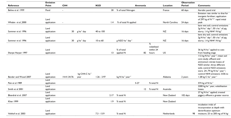
Table 1 Summary of largely overseas piggery production system data. 44
1.1.2 Table of Figures
Figure 1. The DPI&F SIS wind tunnel represents a form of flow through chamber that has been
applied to collect pond and surface emissions. 10
Figure 2. Example of the non-linearity of the gas concentration change under a closed chamber (from
Kroon et al. 2008). 12
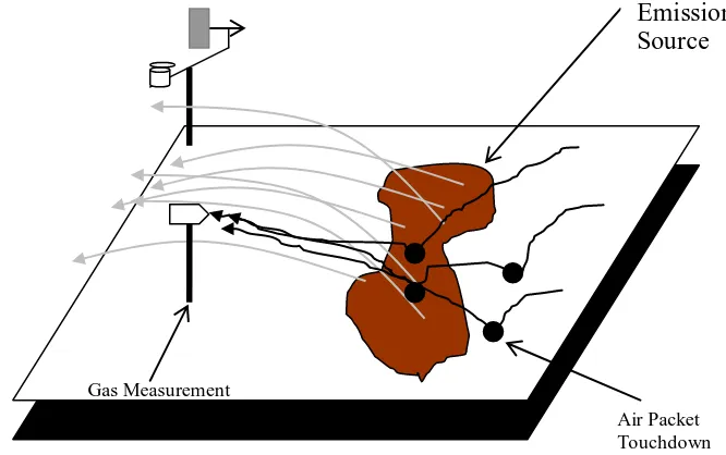
Figure 3. Ammonia emissions measurement using integrated horizontal flux techniques and passive samplers, during a measurement campaign by the DPI&F SIS team. 17 Figure 4. The BLS technique functions by using high resolution meteorological measurements to trace the "packets" of measured gas back to touchdowns within or outside the source area (figure is
a modification of diagrams from Flesch and Wilson 2005). 21
Figure 5. Simulatenous analysis and discrimination of methane (leftmost peak), carbon dioxide (middle peak), and nitrous oxide (right peak) is practical and rapid using GC-MS techniques, as
4
2 Executive Summary
This document details two related literature review conducted as one brief project: a review of greenhouse gas emissions measurement techniques to be applied to intensive pig production; and a review of nitrous oxide emissions and processes from pig production. The review has aimed to be comprehensive and rigorous. However, in order to increase the value to APL, comments and recommendations have been added, including some speculation to allow selection of future directions.
Measurement Techniques and Instruments
In applications where measurements may challenge greenhouse gas assumptions, the most rigorous recognised high accuracy techniques is required
The Backward Lagrangian Stochastic techniques‘ flexibility with regard to emission source and scale is extremely attractive. Advantages include robustness, the body of publications applying it, software support, and modest analytical requirements. The choice of this technique for measurements for the intensive livestock industry in Australia and overseas make the Backward Lagrangian Stochastic method a strong candidate for the primary measurement approach for the pig industry.
Flow through, non-steady state chambers (a chamber placed over an emissions source — such as a deep litter stock pile or suspended over a pond) combined with real-time analysis are probably the best small scale process-based mitigation investigation tool, they allow easy separation of adjacent emissions sources, and also are a critical tool for process evaluations. Most mass balance techniques are more measurement intensive than is desirable, though some techniques may be useful to eliminate the effects of adjacent emissions and to verify the BLS techniques.
Closed path Fourier Transform Infra Red (FTIR) or Tuneable Diode Laser (TDL) instruments will provide the capability to measure emissions adequately in real-time experiments at laboratory, small field scale, and during BLS trials.
Expensive open path tuneable diode laser techniques have proven capability for methane emissions — but instruments are currently not available for nitrous oxide measurement. Gas chromatograph techniques (including GC-MS techniques) are extremely reliable methods suitable for calibration, comparison, and method development roles.
Nitrous Oxide Emissions
Emissions of nitrous oxide occur via both direct and indirect paths.
Direct nitrous oxide emissions can occur from both the nitrification and denitrification processes, and may be delivered through the activity of microbes such as bacteria and fungi, or through purely chemical means.
Denitrification processes are capable of consuming and emitting nitrous oxide.
The major factors controlling emissions from deep litter, effluents, and from effluent/deep litter amended soils are likely to include:
5
Organic carbon availability and quality. This is a mitigation opportunity in that the quantity and ―availability‖ of carbon may be manipulated or altered through managements. Research is required.
Supply of mineral N. This factor is also open to manipulation, and offers potential for the development of mitigation managements. Any management approach that defers nitrate formation or mineralisation until rapid plant uptake is likely will tend to decrease nitrous oxide emissions. Covered anaerobic digesters have advantages in this area, if subsequent nitrogen management steps extract N or allow rapid uptake as nitrate is formed. Systems where effluent or solids ammonia is captured (on smart sorbers or zeolite) or extracted and managed as a high nutrient use efficiency fertiliser would also facilitate a decrease in nitrous oxide emissions.
Soil temperature. Temperature can directly increases denitrification rates, but also via indirect means such as increased respiration rate — resulting in an increase in the volume of anaerobic zones. However, temperature behaviour may not be this simple, as temperature optima do exist. Temperature dependence is more likely to follow a trend of several superimposed relationships. While not readily manipulated in many points in the effluent/deep litter/solids management system, there are likely to be some mitigation opportunities. For example handling, covering, and aeration approaches during composting or stockpiling are capable of altering the temperatures developed. Temperatures in digesters and covered ponds may also be feasible.
Soil pH. The acidity of the soil environment has a controlling influence on nitrification, denitrification, and the ratio of products derived from these processes — directly influencing N2O emissions — and may also influence other nitrogen
transformations, such as immobilisation and mineralisation — that have an indirect influence on emissions. Microbial populations may change or adapt to different pH conditions, and may do so within days. This characteristic is readily manipulated and could form the basis of mitigation development.
Indirect emissions of N2O are likely to be substantial (of the same order of magnitude as
direct emissions), via ammonia volatilisation, deposition, nitrification/denitrification.
A range of reasonably simple mitigation measures to prevent ammonia volatilisation are at a stage where trials may prove some of them practical. These include the use of urease inhibitors, pH modification, use of inexpensive cation exchange materials, and separation of solids from urine.
Piggery effluent nitrous oxide emissions following land application are often larger than those from other waste streams.
Effluent treatment and separating slurry into solid and liquid fractions tends to decrease N2O emissions.
Slurry incorporation and co-application of effluent and inorganic-N sources can greatly increase nitrous oxide emissions.
Nitrous oxide emissions can be particularly problematic from deep litter systems relative to conventional ponds. However Australian data is required.
Permeable pond covers, while potentially valuable in the control of odour, may increase nitrous oxide emissions — though data is scarce.
6
Nitrous oxide emissions from slatted floored housing are likely to be slightly less (in greenhouse gas equivalence terms) than methane emissions. Nitrous oxide dominates GHG emissions from deep litter systems.
Current nitrous oxide emission models are designed for use in soil systems, and tend to be reliant on empirical approaches. The few truly mechanistic models may be over-parameterised. Adaptation to effluent/manure systems would be valuable. Sensitivity analyses could be conducted to remove unwarranted, non critical complexity — revealing the critical factors for manipulation through mitigation managements.
Acknowledgements
7
3 Introduction
Activities across the spectrum of industries are set to encounter considerable pressure for decreased greenhouse gas emissions. While a decision on whether to include agriculture in the Australian carbon trading scheme will not be made until 2013, the lead time to develop the technologies required to make an impact on emissions necessitates that R&D should commence promptly. Even if some portions of the agricultural sector are exempted from the scheme at that time, carbon offset opportunities within the sector may be considerable and a potential source of industry income.
However, even the most basic data is currently not available for the Australian pig industry. For example, emissions data from pig production in Australia has not been collected. Australian Pork Limited has channelled significant funding into specific research areas (capture of methane from covered ponds) related to this deficit, and this will probably be the first relevant data to become available. Availability of the full range of needed data is vital to inform debate around the possible exemption of pig production from the emissions trading scheme. The collection of this vital data may require a substantial investment from the pig industry, and it is therefore important that an appropriate suite of emissions measurement techniques is selected to provide the needed rigorous data at minimum cost.
This literature review will investigate the range of relevant emissions measurement techniques available. A suite of techniques appropriate to the pig industry will be proposed for development of a measurement protocol. The emissions measurement and mitigation issues operating in the realm of pig production have significant commonality with those apparent in other intensive livestock production systems. The review will propose methods with due consideration of the value of a cross industry approach.
Greenhouse gas emissions from intensive livestock enterprises may soon be a major operational consideration. Up to the point of land application, the manure and effluent waste streams from the pig industry are likely to be relatively easy targets for mitigation. Manure and effluent is initially concentrated in sheds, ponds, and spent deep litter or manure solids stockpiles. However, baseline emissions data for the effluent and manure management systems of piggeries is poor or lacking -- both internationally and for Australian conditions.
Relevant data for deep litter systems is almost non-existent. The nitrous oxide emissions that continue after land application of manure/deep litter/or effluent have not been well characterised, and the over-seas data available vary greatly — though it appears that emissions from effluent or manure systems may be much higher than losses from inorganic fertiliser systems with equivalent N applications. Despite the dearth of data, current DOCC guidelines contain techniques for the calculation of piggery manure management emissions — techniques that rely heavily on un-validated emission and conversion factors. In addition to these concerns these calculation techniques do not reward successful mitigation managements. This is a major disincentive to innovation. Ultimately the needs for the pig industry in this area are to accurately quantify the emissions and processes that lead to them, identify the most cost effective points of mitigation, and develop and extend mitigations to producers where required.
8
The literature has a secondary goal to review currently available data on nitrous oxide emissions from the pig industry. While APL, DPI&F, and University of Queensland are currently engaged in a significant research program investigating emissions from piggery ponds, the majority of currently published data is likely to only be available from overseas studies.
4 Emission Measurement Techniques
With the mounting international pressures with regard to climate change and greenhouse gas emissions there has been a dramatic acceleration in the development of techniques for the measurement of emissions. It is now possible to choose from a wide range of approaches, with a range of strengths and different niches for appropriate application.
A number of recent reviews have been conducted. One seeking a broad overview for general applications — and stating the appropriate application context for each (concentrations measured may be 100 times higher than for comparable micro-meteorological techniques. Denmead 2008). Other reviews have sought to recommend approaches for very specific emissions contexts — such as monitoring of the performance of geosequestration (Leuning et al. 2008).
None of these reviews have investigated the range of techniques for applicability to piggery emissions or even to emissions from confined animal feeding operations. However, there have been a range of comparative experimental studies of two or more measurement techniques‘ applicability to the intensive livestock context (Griffith et al. 2008; McBain and Desjardins 2005; Sommer et al.
2004). These studies will be reviewed.
This literature seeks to comprehensively review the available techniques and their applicability in the Australian pig production context, the on farm pig production infrastructure including the land application system — adding the rapidly accumulating science that has been published in the period since the submission of previous more general reviews (e.g. in the 14 months since submission of Denmead 2008).
In selecting techniques appropriate for the piggery context, a range of factors will be considered: The scale of measurement. The scales involved for pig production range from point sources (tunnel ventilation exhausts) and process scales (e.g. small laboratory or field trials concerned with modifiable processes that are readily characterised by measurements at the < 1m scale), through pond and shed scales (10‘s to hundreds of metres in extent), to hundreds or thousands of metres for land application areas.
Practical application. Where if anywhere would the technique fit in to the need to quantifying emissions or process/mitigation development studies in the pig production context?
Accuracy and precision. Cost.
A wide range of techniques are available and will be reviewed: Chamber techniques;
Mass balance methods;
Backwards Lagrangian Stochastic Techniques;
9
4.1 Chamber Techniques
Chamber techniques are the simplest, lowest cost option for portable methods for the capture of greenhouse gas emissions. Implementation varies, but they may be as simple as a dome shaped or cylindrical vessel embedded into a surface from which emissions are to be captured. They are usually of small scale (< 1 m diameter), but have the advantage that they are capable of magnifying changes in concentration of gas in the head space (Denmead 2008) — thus requiring less sensitive analysis techniques or allowing smaller headspace (the air above the surface inside the vessel) concentration changes to be identified.
4.1.1 Flow-Through Steady State Chambers
Flow-Through Steady-State chambers attempt to maintain the concentration of the measured gas in the chamber by a constant known airflow through the chamber.
Emissions are calculated by identifying the difference between the inflow and outflow air concentrations under constant flow conditions. While these techniques are less sensitive when characterising small fluxes than closed chamber techniques, they have the advantage that the constant flow of air can decrease headspace concentration rises that may otherwise inhibit emissions.
While Denmead (2008) comments on the advantages of use of flow through chambers Denmeade‘s review quotes no papers that use this technique. A major disadvantage of flow through steady state chambers is that related to the pressure gradient that may be induced by the air flow through the chambers (Rochette and Hutchinson 2005). Even small gradients of less than 4 Pa have been demonstrated to result in a several fold increase in CO2 emission (Kanemasu et al. 1974). Indeed, it has been demonstrated that pressure gradients must be maintained below 0.2 Pa for accurate determinations (Fang and Moncrieff 1996). The theoretical advantages of these chambers over non-steady state or non-flow through techniques theoretically include: an ability to maintain headspace gas species at pre-deployment concentrations, control of temperature, and control of humidity. However, it has proven difficult or impossible to capitalise on the theoretical advantages of this form of chamber in many situations. If emissions are large relative to the background atmospheric concentrations, it may be impossible even to maintain headspace gas concentrations at close to pre-deployment concentrations.
However, this method, which is similar to wind tunnel techniques, has recently been applied by Blunden and Aneja (2008) to piggery lagoons overseas in order to determine ammonia and hydrogen sulphide emissions. In addition, the SIS team has used this technique extensively to determine odour, hydrogen sulphide, and other gaseous emissions from piggery ponds and other intensive livestock industry sources. Emissions may be calculated as follows:
Flux (kg m-2 s-1) = v ( g,0 - g,i)/A, Equation 1
where the volume flow rate is designated v (m3 s-1), outflow and inflow gas concentrations are g,0
and g,i (kg m-3), and A (m2) is the area of the surface contained under the chamber.
10
Figure 1: The DPI&F SIS wind tunnel represents a form of flow through chamber that has been applied to collect pond and surface emissions.
4.1.2 Non-Flow-Through Non-Steady-State Chambers
A recent review (Rochette and Eriksen-Hamel 2008) of data from non-flow through non-steady state chamber studies (one of the two forms of closed chambers) indicated that while the vast majority of nitrous oxide (N2O) emissions studies have been conducted using these techniques (356
studies reviewed), the data quality of these studies is often poor: poor in terms of absolute measurement accuracy, and poor in terms of methodology. In more recent years, however, the quality of these studies has improved — and the reviewers indicated six factors that can be controlled to improve the quality of N2O flux measurements:
1. Use insulated and vented base-and-chamber designs. 2. Avoid chamber heights lower than 10 cm,
3. Insert the chamber into the emissions source a minimum of 50 mm,
4. Use pressurized fixed-volume containers of known efficiency for air sample storage (i.e., avoid plastic syringes),
5. Include a minimum of three discrete air samples during deployment, including one at time zero, and
6. Test nonlinearity of changes in headspace concentration with time for estimating dC/dt at time zero.
Indeed Rochette and Eriksen-Hamel (2008) indicate a list of chamber characteristic and technique issues that should be considered in the implementation of any chamber measurement campaign:
Surface disturbance related to insertion of chambers into surfaces, and diffusion of gas around this barrier (leakage). Insertion into soils should exceed 120 mm per hour of deployment. There are advantages of a semi-permanent base, over which the chamber is fitted at measurement time.
The height/measurement period ratio of the chamber should exceed 400 mm h-1.
Chamber area to perimeter ratio determines the importance of leakage relative to emissions — it is therefore recommended that cylindrical chamber diameters exceed 400 mm.
Duration of deployment determines the degree of perturbation of soil and air temperature, humidity, gas leakage, and inhibition of emissions. Deployment durations should ideally be kept to less than 40 minutes.
11
Venting — pressure must be able to equalise, without significant leakage occurring. Quality control of air samples — since chamber studies are often associated with off-line analysis rather than in-field analysis. This includes restricting storage periods. However if exetainers are used it has been shown that < 1.5 % change in concentrations will be observed. Where other techniques are applied, a container life/contamination study should be conducted.
Fixed volume sample containers are to be preferred, followed by glass syringes. Plastic syringes are not desirable.
Positive pressure in sample containers minimises contamination risks.
Use non-linear modelling of the concentration increase within the chamber where a linear increase with time is not observed. This requires four or more samples to be collected, allowing extrapolation to time zero emission should significant emission inhibition be detected.
Samples should be taken as soon as possible after deployment time.
Ensuring that reported emission rates exceed the detection limit or are simply reported as sub-detection, rather than quantified.
Correct gas analysis for changes in gas temperature during analysis according to the ideal gas law (Rochette and Hutchinson 2005).
Closed chamber techniques have effectively been evolving over several decades, and their value as a means of monitoring relative changes (for example with different treatments in process and mitigation studies) is well established (Rochette and Eriksen-Hamel 2008).
In its simplest form, emissions are calculated according to the following formula (Denmead 2008):
Flux = (V/A) d g /dt Equation 2
where the volume is designated V (m3), gas concentrations are g (kg m-3), and A (m2) is the area of
the surface contained under the chamber. The term t represents time (s). While not explicitly stipulated by the formula, previous applications of the method have tended to use a linear relationship to model the increase in gas concentration over time (e.g. Hendriks et al. 2007; Ruser et al. 1998). However, there is credible evidence that the slope of increase of gas concentration with time (d g /dt) (Healy et al. 1996; Kroon et al. 2008) is best assumed to be non-linear as increasing
12
Figure 2: Example of the non-linearity of the gas concentration change under a closed
chamber (from Kroon et al. 2008).
Rather than being portable many of the chamber designs are set in place and caused to (automatically) open and close. This is very unlikely to be suitable for trafficked areas in the intensive livestock context. Also, it is likely that this approach would violate some of the heat transfer and shading conditions for good measurements that have been recommended (Rochette and Eriksen-Hamel 2008).
Chamber NFT-NSS techniques remain a key method in the arsenal — fitting situations where no other methods are available. They naturally exclude emissions from other sources, they have low power requirements compared to many other techniques, and they provide greater measurement sensitivity than more expensive techniques. These techniques are also particularly adept at detecting relative treatment differences, and are well suited to process-based mitigation studies — and are capable of measuring emissions at small scale. While Denmead (2006) indicated that there was a factor of 2 variations in emission values for N2O from six chambers, the daily means of the emission values from the chambers was very close to those measured by the aerodynamic technique. Where sufficient replicate chambers are applied it appears that they can be used to quantify emissions from larger sources — suitable for situations where confounding emissions from adjacent sources are a significant problem, or where maximum measurement sensitivity is required.
4.1.3 Flow-Through Non-Steady-State Chambers
13
Observation: FT-NSS chambers combined with real-time analysis are probably the best small scale process-based mitigation investigation tool.
Since the characteristics of these chambers are otherwise similar to those for non-flow-through non-steady-state chambers, the same range of advantages and disadvantages apply with the added advantage of being able to continuously monitor concentrations in real time.
4.1.4 Application Contexts
Given appropriate methodology chambers are known to produce accurate and acceptable results, though many studies have to date been conducted inadequately, or documented inadequately (Rochette and Eriksen-Hamel). The small spatial extent of chamber techniques (e.g. cylindrical chambers with diameters of 400 mm; Rochette & Eriksen-Hamel 2008) suggests a significant disadvantage for larger scales.
However, it is known that replication can overcome this issue where chamber use is necessary, or where chambers have been deployed for another purpose but information is also required at a larger scale. For example, a factor of two variation in emission values for N2O from sugar cane soils with six chambers was observed, though the daily means of the emission values from the chambers was very close to those measured by the aerodynamic micrometeorological technique (Denmead et al. 2006). Comparisons were less encouraging in this case for methane emissions, due to spatial variability or detection limit issues, however, similar successes with replicated chamber studies are also reported elsewhere (Laville et al. 1999).
Some issues to note in the application of these techniques to pig industry research:
Conventional shed emissions. Practical applications in this context are not immediately evident.
Deep litter sheds. Application of this technology within deep litter sheds to measure emissions from the floor space is likely to be practical, inexpensive, and may enable elimination of the influence of other nearby sources. Where nearby sources are not significant or can be eliminated other techniques detailed later in this review may be more suitable.
Ponds. These types of technologies have already been applied to measuring emissions from ponds, and technologies could be similar to those associated with the DPI&F SIS wind-tunnel. While there is likely to be an application for these techniques in eliminating the influence of adjacent emissions sources, it is also probable that other mid scale approaches detailed in this report will be less adversely affected by spatial variability, and will entail lower labour costs due to the need for high replication.
Sludge and solids stockpiles. Similar to the comments above, where discrimination of sources is required, chamber techniques may have application in this context for fairly impermeable stockpiled materials (Pattey et al. 2005). However, where stockpiled solids have significant gas permeability non-steady-state chambers are likely to be completely inappropriate, due to a strong effect in inhibiting evolution of gasses (Sommer et al. 2004). Land application areas. Similarly to above, measurements can be conducted where sufficient replication is applied (Denmead et al. 2006; Laville et al. 1999).
14
Recommendation: NFT-NSS chambers are a key technique for process investigations and development of mitigations in laboratories. They may also be used to separate emissions sources where these adjacent emissions may otherwise be intermingled and expensive or impossible to differentiate.
4.1.5 Strengths and Weaknesses
Chamber methods encompass a range of techniques that are quite inexpensive relative to the other options reviewed in this document. These techniques are extremely portable, and do not require fast response analysers, nor do they require highly sensitive analysers (concentrations measured may be 100 times higher than for comparable micro-meteorological techniques. Denmead 2008).
Weaknesses associated with pressure differences that may result in large errors (Denmead 1979) can be overcome through appropriate venting (Meyer et al. 2001; Rochette and Eriksen-Hamel 2008) or the use of electronic pressure and flow control (Denmead 2008). Turbulence in the chamber may affect the flux (DenmeadReicosky2003), or the flux measured may not reflect the wind speed derived flux from outside the chamber. The solution appears to be to relate emissions to a regular wind speed pattern or to a relationship function as described in Denmead (2008).
The short recommended duration of measurement for NSS chambers implies a large labour requirement for measuring piggery enterprise components where there are large diurnal (Jury et al.
1982), seasonal, and nutrient input-related variations that must be characterised by in a comprehensive measurement campaign (Kroon et al. 2008). Indeed Denmead in his review (2008) points out that due to diurnal cycles – the minimum measurement collection period should be 24 hours of contiguous measurements.
4.2 Mass Balance Techniques
These analytical techniques are guided by the principle:
GHG emissions = GHG exit from area - GHG entry into area, Equation 3
Or more formally, mean horizontal flux Fh (kg m2 S-1) at level z for unit width:
Fh,z = mean over time(uz( g,z- g,u)) Equation 4
15
Recommendation: In applications where measurements may challenge greenhouse gas assumptions, we recommend that the most rigorous approach involving the use of fast response anemometers.
g
g u
u Equation 5
However, there is a significant error in this formula, which would more accurately represented as:
g g
g u u
u ' ' Equation 6
where, u’represents the deviation from the mean of wind speed, and likewise g‘ the deviation from the mean for gas concentration, and the term u' 'grepresents a turbulent diffusive flux in the
upwind direction. The magnitude of u' 'g is between 5 to 20 % of the value of u g(as reviewed
by Denmead 2008) as confirmed in field trials and wind tunnel experiments (e.g. Desjardins et al.
2004). Denmead (2008) recommends a decrease in the horizontal flux estimated by 10 to 15 % or the use of fast response anemometers (Desjardins et al. 2004), such as 3d sonic anemometer apparatus.
The turbulent diffusion flux, however, is the only complication to what is otherwise a fairly simple theoretical basis for the ―closed‖ and ―open‖ forms of mass balance methods.
Some ambiguity is evident in the classifications of techniques described by several of the most recent and comprehensive reviews. Leuning et al. (2008) refers to ―Three dimensional transport‖ measurement systems, and includes in this measurement methods that are certainly mass balance methods — referring to the range of these mass balance techniques as ―integrated horizontal flux methods‖, including together under this title methods that Denmead (2008) refers to as ―closed‖ and ―open‖ mass balance methods. McGinn‘s (2006) separation of ―integrated horizontal flux‖ techniques seems more logical, discussing ―mass difference‖ methods and ―integrated horizontal flux‖ techniques.
4.2.1 Closed or Mass Difference Systems
Closed mass balance approaches seek to measure concentrations both upwind and downwind of a source by means of a grid of samplers, and are suitable for small well defined source areas. They are suitable even for source areas of heterogenous character (Denmead 2008) or complex topography (Leuning et al. 2008). A key advantage of these methods is their ability to represent three dimensional transport (Leuning et al. 2008), making them suitable for measurement of emissions from ponds where there is significant wind disturbance over the surface, where one dimensional methods (such as the flux gradient methods described below) are known to fail (Wilson et al. 2001). When applying these methods, wind velocity (speed and direction) is measured and emissions samples analysed at enough sampling heights to define the concentration profile from the ground surface to the full height of the emission plume.
16
These methods have been used by Denmead et al. (1998) to measure emissions of CO2, CH4, N2O from landfill. They have also been applied to measure methane emissions from penned and free ranging cattle and sheep (Harper et al. 1999; Leuning et al. 1999), and nitrous oxide emissions from a grazed pasture (Denmead et al. 2001). The enclosed areas investigated by Harper et al. (1999) and Leuning et al. (2001) were square with 24 m sides, with measurement conducted at 0.5, 1, 1.5, 3.5 m, or 0.5, 1, 2, and 3.5 m above the ground.
4.2.2 Open or Integrated Horizontal Flux Systems
Integrated horizontal flux techniques (Denmead et al. 1977) utilise a single tower upwind (or known background concentrations), and a single tower downwind of the source (McGinn 2006), and configuration in relation to wind direction determine the completeness of emission characterisation. These techniques are most appropriate in situations of limited upwind source and uniform surface flux and are suitable for measurement of emissions from animal herds and buildings, and from manure management activities such as spreading, effluent lagoons, manure piles, and waste sites (Denmead 2008).
Integrated horizontal flux techniques have been applied to measure emissions from cattle manure stockpiles (Sommer et al. 2004), from grazing cattle (Griffith et al. 2008), from dairy cow herds (Laubach and Kelliher 2005; Laubach and Kelliher 2004), and from grazing sheep (Leuning et al.
1999). Integrated horizontal flux techniques are sometimes used as a reliable reference technique for comparison to other methods (Sommer et al. 2005). Integrated horizontal flux techniques have proven ideal for measurement of manure storages and other point sources (McGinn 2006).
As for mass difference techniques, it is necessary to measure emissions downwind at sufficient height to define the shape of the concentration profile to the top of the emission plume.
17
Figure 3: Ammonia emissions measurement using integrated horizontal flux techniques and passive samplers, during a measurement campaign by the DPI&F SIS team.
18
excess of 6 m. In general, these open mass balance techniques encounter difficulties where wind direction shifts outside a pre-set limit. Where uniform circular emission plots are feasible, this problem can be eliminated by locating a sensor tower at its centre, thus ensuring that the length of fetch is always the same (Beauchamp et al. 1978). In addition to this pioneering work on ammonia emissions from sewage sludge application, the technique has been applied to other emission situations (examples listed in Denmead 2008). Recently the circular source variation of the IHF technique was successfully was to ammonia emissions from piggery effluent applied in a circular plot (Warren et al. 2006). Accuracy deteriorates with decreasing plot radius, and the recommended minimum radius for the technique is 20 m or more, providing accuracy to within 20 % for ammonia volatilisation (Wilson and Shum 1992).
An evolution of the integrated horizontal flux technique provided by Wilson et al. (1982) allows gas flux to be determined from measurements of wind speed and gas concentration at just one height above the surface. This development is reliant on the observed relationship that
u
/
Flux
is almostconstant at a specific height (ZINST) despite changes in stability conditions. The height of ZINST is dependent on plot radius and surface roughness (z0). The authors of this development also provided a procedure to estimate errors due to selection of inappropriate ZINST values (e.g. due to poor values of z0). The method was relatively insensitive to errors related to inaccuracies in z0, with these error values being less than or comparable to errors for the more measurement intensive circular plot techniques (e.g. Wilson and Shum 1992).
4.2.3 Application Contexts for Mass Balance Techniques
Observations on the application of these techniques to the pig industry:
Overall emissions from conventional and deep litter sheds. Mass difference mass balance approaches may be effective in measuring emissions from sheds. Sensitivity to disturbance of air flow over the sheds themselves is unknown, and may increase plume heights, or result in other negative effects. The technique should be capable of eliminating the effects of adjacent sources. Integrated horizontal flux techniques are unlikely to be applicable due to the heterogeneous nature of the source areas.
Ponds. Mass difference techniques have been successfully applied to pond emission measurement. Integrated horizontal flux techniques may be applicable if disturbance due to banks and structures is not significant. Ponds are unlikely to be circular sources, so these latter techniques would not be able to take advantage of the simplifications that a circular source might enable, and fetch length to the downwind measurement tower will vary with wind direction.
Sludge and solids stockpiles. Both forms of mass balance techniques are likely to be applicable to these measurements. The integrated horizontal flux method requires more ingenuity in this application, however, the technique has been applied to a circular plan stockpile with good results, using a weather-vane-like upwind and downwind sensor apparatus suspended above the stockpile (Sommer et al. 2004).
Land application areas. Small to moderate plot sizes (0 to 90 m) could be investigated by either one or other of the mass balance techniques, based on comments in the Denmead (2008) review and other reviewed literature.
19
Recommendation: Most mass balance techniques are more measurement intensive than is desirable. However the ability of mass difference techniques to eliminate the effect of adjacent emission sources may be valuable, and integrated horizontal flux techniques provide a relatively simple technique to which to compare emissions measurements conducted using other techniques. These advantages may make these techniques unavoidable in some circumstances, however, the measurement efficiency of some of the following techniques make mass balance methods less attractive.
4.2.4 Strengths and Weaknesses of Mass Balance Techniques
Mass balance techniques are appropriate for small to mid scale source areas with well defined boundaries (several metres to 90 m according to Denmead 2008). Both homogenous and heterogeneous emissions source measurements can be accommodated with one or other mass balance approach. As Denmead (2008) notes that both homogenous and heterogeneous sources can be measured using:
closed path analysis instruments in combination with mass difference measurement techniques
open path measurement instruments in combination with an integrated horizontal flux approach
Integrated horizontal flux techniques employing closed path single point measurement instruments require a homogenous source distribution.
Rapid response instrumentation is not required. However, slow response instrumentation requires the application of a correction for diffusive flux (decrease estimated flux by 10 to 15 % as discussed in section 2.2). This type of correction is not necessary where fast response instrumentation is applied (Desjardins et al. 2004). No assumptions are made about the wind profile or stability characteristics of the system.
Circular plots offer a considerable simplification of the integrated horizontal flux technique, overcoming the need to continuously monitor wind direction — since fetch distances are always equal. Where this is not possible measurements and post possessing is greatly complicated, and wind direction may render tower placement in a given configuration completely inappropriate.
Mass balance methods are most likely to be effective where strong contrast exists between background concentrations and wind concentrations exiting the plots.
At least 5 profile measurements are required over pastures, or fallow soil (Denmead 2008). However more are probably required where surface airflow is disturbed (such as over a banana plantation, Prasertsak et al. 2001). This suggests that greater profile heights and more samplers may be required for measurements around sheds and ponds.
4.3 Backward Lagrangian Stochastic Techniques
20
enterprises apart from large effluent or solids re-use areas. This latter problem was recently explored for a cattle lot-feed (Baum et al. 2008).
The backward Lagrangian stochastic technique (BLS) is one means of overcoming these difficulties and introducing significant measurement flexibility.
The ―Lagrangian‖ of a dynamic system is equal to system kinetic energy minus potential energy. Where the conditions of Lagrangian Mechanics apply, the motion of particles in a system can be represented (using the Euler-Lagrange equation) if this Lagrangian value is known.
A Lagrangian model of atmospheric dispersion can be used to calculate the flux of a gas given measurements of atmospheric turbulence and concentrations of the gas of interest in air at any height downwind — under any stability condition (Flesch et al. 2004; Flesch et al. 1995).
This translates, in practical terms, to considerable measurement flexibility, and has the added advantage that the technique may be applied with line averaged concentration measurements or with point measurements. The method is likewise applicable to both point and area sources.
The BLS technique is applicable to well defined source areas of moderate size, and any shape — and has already proven very applicable in the measurement of emissions from various beef lot-feed sources (Loh et al. 2008).
Lagrangian mechanics is used to trace detected ―air-packets‖ through their trajectories back from the sensor to the emissions source, using fast response anemometer data (10 Hz measurements; Figure 4). A large number of these simulations are conducted (commonly 50,000). "Touchdowns" are noted as being inside or outside the source area of interest, as the vertical velocity of the particle calculated. The following relationship is used to describe the system:
,
/
2
)
/
1
(
)
/
(
gF
0 simulatedN
w
0 Equation 7F0 is surface flux density, N is the number of particles simulated, w0 is the vertical velocity of particles at touchdown. The surface flux density is derived from:
,
)
/
/(
)
(
, 00 g gb g
F
simulatedF
Equation 8where g,brepresents the background gas concentration. The application of the BLS technique is greatly streamlined and simplified by the use of the Windtrax model (Crenna et al. 2008).
Inputs to the model (Crenna et al. 2008) include the surface roughness height (z0), source area
geometry, and the three dimensional location of the gas sensor, wind speed, direction, and turbulence statistics such as the Obukhov length (L) and friction velocity u*.
21
overdetermination techniques, a CV of 10% has been achieved for ammonia emissions measurement from grazed cattle (Denmead et al. 2004).
Figure 4: The BLS technique functions by using high resolution meteorological measurements to trace the "packets" of measured gas back to touchdowns within or
outside the source area (figure is a modification of diagrams from Flesch and Wilson 2005).
4.3.1 Robust Measurement
Underlying Lagrangian dispersion modelling and the BLS technique are assumption of the Monin-Obukhov hypothesis (Monin and Monin-Obukhov 1954). This theoretical base suggests that over flat terrain, atmospheric surface layer turbulence is determined by a few key parameters, including height, buoyancy, kinematic surface stress, and surface temperature flux (Kaimal and Finnigan 1994). These assumptions are least satisfied during severe atmospheric stratification or during transition periods such as sunrise and sunset. Estimates conducted during periods of extreme stability may also be problematic (Flesch et al. 2004).
Flesch and Wilson (Flesch and Wilson 2005) suggest that where the terrain is ―tolerably‖ homogenous and amenable to the assumptions of Monin-Obukhov theory, the BLS approach can be applied.
In fact, research has already gone a long way to demonstrate just how tolerant and robust the BLS technique is. For example, it has been demonstrated that the technique is insensitive to obstructions between the measurement point and the source — so long as the obstruction was placed more than 25 times it's height from the measurement point (McBain and Desjardins 2005). Measurements of ammonia emissions from the banks surrounding piggery ponds (Dzikowski et al. 1999) have been found to be quite accurate (Flesch and Wilson 2005), within 15 % of measurements conducted using an integrated horizontal flux technique during largely overlapping time periods (McGinn and Janzen 1998). The departures from ideal Monin-Obukhov similarity assumptions caused by the banks of the piggery pond had an insignificant effect on final measurements (Flesch and Wilson 2005).
Divergence from Monin-Obukhov similarity assumptions at the emission source has also been investigated. The effect of obstacles at the source could be overcome by placing the detector an
Emission Source
Gas Measurement
22
appropriate distance downwind (Flesch et al. 2005) — suggesting that measurements of shed sources may be effective. Other options for these types of measurements are likely to be far more expensive (e.g. the intensive sampling required for mass difference techniques on this relatively large scale). A combination of the BLS technique with tracer gas release may be ideal.
Near continuous data sets can be obtained by placing sampling equipment within an emission source area, producing superior data for some source configurations, including beef lot-feed pads (Flesch et al. 2007).
The nature of the BLS model is that measurements conducted at the margin of the emission plume are least likely to produce accurate flux estimates. Adjacent emission sources that disrupt the uniformity of the background concentrations introduce the need for additional sampling and measurement. For example a study has been successfully conducted that separated emissions from adjacent grazed and ungrazed paddocks (Denmead et al. 2004).
One criticism of possible numerical errors in some BLS models (Cai et al. 2008) may simply indicate that the impressive performance of the BLS approach demonstrated in comparison trials could be improved upon. Flesch and Wilson (Flesch and Wilson 2005) suggest that the upper limit of single time-point based flux estimates with this technique is around ± 10 % (assuming perfect wind statistics, which do not exist). Where continuous measurements are conducted with multiple sample points or multiple sample lines, the upper limit of potential for accurate representation is even better. Ultimately the limitation may be the accuracy of the wind statistics available.
4.3.2 Application Contexts for BLS Techniques
As indicated by Denmead (2008), this technique is particularly suited to measurement of intensive animal systems and land application areas. Thus it is one of the primary techniques recommended in this review -- for ponds, sheds, and effluent/solids re-use areas. Pilot trials in conjunction with tracer release (Griffith et al. 2008; Sneath et al. 2006) will help ensure accurate representation of disturbed emissions sources.
Importantly, the technique is already in use in Australian studies of intensive livestock emissions from other industry sectors (beef lot feeding, Loh et al. 2008; McGinn et al. 2008).
4.3.3 Strengths and Weaknesses of BLS Techniques
The mounting body of experimental evidence suggests that while assumptions of appropriate conditions for MOST theory are made for the application of the BLS technique, the technique is robust and measurements conducted using it are accurate. Applications to date have been demonstrated for piggery ponds and beef lot feeding.
The technique is sensitive to poor sampling position relative to the plume, and measurements conducted close to the margins of plumes should be discarded. Similar data filtering should be applied to periods of extreme atmospheric stability, transition periods, and periods of extreme atmospheric stratification.
23
Recommendation: The source and scale flexibility, robustness, body of publication, software support, modest analytical requirements, and choice of this technique for measurements for the intensive livestock industry in Australia and overseas make the BLS method a strong candidate for the primary measurement approach for the pig industry.
The availability of the Windtrax model is also a significant advantage to the implementation of the BLS technique (Crenna et al. 2008).
4.4 Landscape Scale Micrometeorological Methods
Micrometeorological approaches apply where fluxes are nearly constant with height and concentrations change vertically but not horizontally. These approaches are therefore unlikely to apply to pig production and other intensive livestock systems, except where effluent, manure, or manure solids are land applied very broadly in homogenous flat terrain.
The area contributing to the flux measured by a technique is called its ―footprint‖. Under the limitations of micrometeorological techniques, the footprint must logically be smaller than the homogenous source area, and superimposed on it. The footprint of the source contributing to measured gasses at a height z is strongly influenced by surface roughness and thermal stability (Denmead 2008). Several rules of thumb have been observed to apply (Leclerc and Thurtell 1990; Schuepp et al. 1990), producing conditions where flux is nearly constant with height of z, and representative of the flux at the surface (Denmead 2008):
In neutral conditions 85 % of the flux measured at z originates from within 100 z upwind, with the biggest contributions coming from around 10 z. The practical fetch to height ratio to use is 100:1.
In unstable conditions the footprint is somewhat smaller, however, in practical terms the appropriate fetch to height ratio to use is once again 100:1.
In stable conditions this footprint is much larger. Fetch to height ratios expand to 200 to 350:1.
In effect this means that opportunities to use these techniques for the pig industry are probably restricted to homogenous (in terms of topography, soil, and management), large land application areas — where it may be possible to select a fairly regular measurement area with hundreds of metres of upwind extent.
Techniques include eddy covariance, eddy accumulation, and relaxed eddy accumulation.
4.4.1 Eddy Covariance
In many ways, eddy covariance techniques are the most direct way to measure emissions: they determine the vertical flux at the point of measurement, are unaffected by the stability considerations that must be applied to many other methods, and do not require simplifying assumptions (Denmead 2008).
24
The problems related to greenhouse gas emissions measurements using this technique are:
Complications related to simultaneous fluxes of heat and water vapour. Constant sample temperatures can be used to eliminate this issue in closed path analysis using heat exchangers or minimum tube lengths (Leuning and Judd 1996). Air sample dryers can likewise be used to eliminate water vapour issues (Laville et al. 1999).
Since high frequency gas analysis and meteorological data is required there is a need to account for lag between vertical wind measurements and gas concentrations.
While closed path analyses seem to be the only current option, the sample tubes conducting gas to the instrument have the effect of damping important concentration fluctuations due to wall sorption behaviour (Ibrom et al. 2007). Advice on how to deal with this issue has been published (Leuning and Moncrieff 1990) and also means of estimating the impact of this behaviour (Leuning and Judd 1996).
The general difficulty with these ―landscape scale‖ methods — large fetch lengths relative to sampling heights.
Selection of vertical and wind direction alignment of the sonic anemometer to prevent negative effects of flow distortion errors around the instrument given that wind direction will vary (Coppin and Taylor 1983; Kaimal et al. 1990).
The influence on flow due to neighbouring equipment and structures (Moore 1986, as cited in Denmead 2008)
The extremely high frequency of sampling required.
In stable conditions (e.g. night) eddy covariance techniques were found to be preferable to flux gradient techniques for nitrous oxide emissions from grazed pastures (Phillips et al. 2007). However, error due to the micrometeorological technique and analysis combined were about 60 % at night. Similarly errors determined by (Laville et al. 1999) were about 25 % for 15 min flux estimates for N2O using eddy covariance and flux gradient measurements.
4.4.2 Eddy Accumulation
Researchers developed this technique as a solution to the high frequency of sample analysis required to conduct eddy covariance studies (sample analysis required 10 times every second, McInnes and Heilman 2005). Samples are collected with apparatus that collect separate updraft and downdraft samples, proportional to the magnitude of their vertical velocities — that are then analysed (Desjardins 1972). While this solution appeared attractive, there was a practical difficulty in maintaining constantly proportional sampling throughout the range of vertical wind-speed fluctuations that occur in the field (McInnes and Heilman 2005). The relaxed eddy accumulation technique is this methods successor.
4.4.3 Relaxed Eddy Accumulation
The concept behind this approach is similar to that for the eddy accumulation technique, however, sampling proportional to the vertical wind speed is not required. Samples are simply collected at constant flow into one of two bins representing updrafts and downdrafts.
High precision measurements of vertical wind speed are required, and offsets between sample collection times and wind speed measurements cannot be eliminated with latter processing (Leuning
25
, )
(
ft m ft m d d
F w a w a Equation 9
where over-bars represent time means, is a proportionality factor, is the mixing ratio for the gas analysed, dais the density of dry air, w is the standard deviation of the vertical wind velocity, f is the mass flow rate of dry air, t represents the sampling period, and
m
andm
represent themasses of upward and downward accumulated gas to be analysed.
Published literature suggests that the relaxed eddy accumulation technique is a viable alternative to eddy covariance methods for greenhouse gas measurement (McInnes and Heilman 2005). The fact that measurements are conducted at a single height rather than several heights is a slight advantage over flux gradient techniques (described below).
Recently, the relaxed eddy accumulation technique has been applied in an aircraft mounted application to measure landscape scale methane emissions (Pattey et al. 2006).
4.4.4 Flux Gradient Methods
These methods are reliant on an analogue of gas diffusion — gas parcel diffusion. While diffusivities of molecules can be around 0.00001 m2 s-1, parcel diffusions, however, will be on the order of 0.1 m2
s-1, with this diffusion constant being represented by Kg (Denmead 2008). The value of Kg is
influenced by wind speed, height of the point of interest, atmospheric stability, and "aerodynamic roughness". The result of these interactions is that Kg is site and example specific — it must be determined in situ. The underlying relationship for gas emission flux is:
, / z K
Fg g g Equation 10
and similar equations apply to fluxes of heat and momentum (H, ), where the eddy diffusivities are represented by Khand Km:
, / z K
d c
H p a h Equation 11
,
/
z
u
K
d
a m Equation 12where is the potential temperature of the air (the temperature of an air parcel if it was brought to a standard reference pressure, 1 atmosphere, without heat loss or gain) and cpis the specific heat of air at constant temperature (energy required to raise the temperature of a mass of air by a unit of temperature).
In the aerodynamic method the gas concentration and the flux of momentum between the atmosphere and the surface are used to estimate gas concentrations. The diffusivity in Equation 10 is substituted as follows:
,
/
* g
g
ku
z
26
where k is von Karman‘s constant, the function g represents the stability conditions of the
atmosphere (as summarised in Prueger and Kustas 2005), and u* is the friction velocity. Gas concentrations are usually measured at two levels, and the difference between the concentrations at the two heights used in calculations.
Significantly, this technique allows measurement from smaller plot sizes (1-2ha) than from eddy covariance techniques. Since sonic anemometer readings are not required, anemometer readings can be conducted with other devices — that may be mounted closer to the ground surface. This leads to a smaller fetch — and small footprint (smaller plot size)(Wagner-Riddle et al. 2005). Since 3-d sonic anemometry is not required, emissions measurements using cup or 2-d anemometers can also be conducted during fog, dew, and rain. Since synchronisation of high frequency anemometer and gas analysis is not required, buffering effects and high frequency damping of gas concentrations in sample tubes is no longer important — and long sample tubes can be used with closed path analysis techniques (Denmead 2008). McGinn (2006) suggests that aerodynamic methods may be appropriate for effluent pond measurements — but only large lagoons of appropriate footprint (given the above footprint information, presumable larger than 2 ha, which are probably rare or non-existent in the pig industry), and the method is probably inappropriate for any other pig industry point source. While not recommended by McGinn (2006) his review indicates that aerodynamic methods have been applied by a number of researchers in relevant contexts: piggery effluent ponds (Harper et al.
2000; Harper et al. 2004) manure holding facilities, dairy cow emissions from a grazed field — though with additional corrections (Laubach and Kelliher 2004).
A major disadvantage of using aerodynamic techniques is inaccuracy when wind speeds are low — leading to inaccurate estimates of wind speed gradients and large errors in calculated emission fluxes (McGinn 2006). However, in terms of measurements for the pig industry, possibly the greatest downfall of the methods is their suspected inaccuracy due to the difference between the real values of Kg and Km which are normally assumed to be equal or comparable in calculations (estimated emissions only 0.6 of true emissions, Flesch et al. 2002).
While the aerodynamic method uses momentum as a tracer, the same sort of approach can be applied to other tracers: water vapour, CO2, and heat (Tracer methods). The Bowen ratio or energy balance method uses energy as the tracer flux.
Net radiation, or the energy balance, is dependent on the flux density of sensible heat from the surface to the atmosphere, the flux density of latent heat (due to evaporation), the flux density of heat into the soil's surface, and storage of energy. The technique requires measurement of the flux density of heat into the soil, usually with soil heat flux plates. Where accuracy is important, measurements of other sources and sinks of energy are required. The result is a suite of high accuracy measurement requirements.
27
Recommendation: Micrometeorological approaches apply where fluxes are nearly constant with height and concentrations change vertically but not horizontally. These approaches are therefore unlikely to apply to pig production and other intensive livestock systems, except where effluent, manure, or manure solids are land applied very broadly in homogenous flat terrain. Relaxed eddy accumulation may be applicable to large land application areas. The accuracy questions associated with some micrometeorological approaches to greenhouse gas quantification would rule them out of consideration (flux gradient and eddy covariance).
Experienced practitioners with any of these flux gradient methods recommend a suite of sampling approaches to minimise errors between measurements at the different heights, including the use of reference gas cells in analysers and using the same analyser for all heights of analysis by switching gas supplies (Wagner-Riddle et al. 2005).
In unstable atmospheric conditions (e.g. day), it appears that the aerodynamic technique (using friction velocity measured by eddy co-variance) is the most appropriate flux gradient approach, and in stable conditions (e.g. night) eddy covariance techniques were preferable to flux gradient techniques for nitrous oxide emissions from grazed pastures (Phillips et al. 2007). Error due to the micrometeorological technique and analysis combined were about 25 % during the day to 60 % at night. Phillips et al. (2007) were forced to correct for footprints that were larger than plot sizes, and filter data based on factors like wind direction — the complex nature of this calculation may be a deterrent to further use of the technique in similar applications in the pig industry. Similarly errors determined by (Laville et al. 1999) were about 25 % for 15 min flux estimates for N2O using eddy covariance and flux gradient measurements.
4.5 Online, Offline, Closed Path or Open Path Analysis?
One of the decisions to be made regarding the application of any of the above micrometeorological, BLS, mass difference, or integrated horizontal flux techniques is the type of gas analysis technique to apply.
Offline technologies, where gas samples are collected and transported to an analyser are applicable for some types of studies. Indeed gas chromatography has been applied as a ―gold standard‖ comparison or as the primary line of analysis in range recent studies at different scales (Harvey et al.
2008; Mkhabela et al. 2006; Skiba et al. 2006). Offline analysis via gas chromatography is adaptable to the range of scales, though other techniques are less labour intensive where large numbers of samples are collected a long way from the laboratory. Gas chromatography may be the most appropriate means of measuring some common tracer gasses such as SF6 (McGinn et al. 2006).
A recent review appeared to suggest that off-line analysis (possibly gas chromatography) remained the standard for chambers studies, though this issue was not discussed directly (Rochette and Eriksen-Hamel 2008). While the DPI&F team has several conventional gas chromatographs, the team‘s Gas Chromatograph-Mass Spectrometer equipped with a PLOT column for greenhouse gas analysis has proven to have added advantages with respect to simultaneous analysis and discrimination of the range of gases in a single sample (Figure 5). This GC-MS technology is not regarded as portable and is therefore suitable for off-line analysis and real time analysis only where laboratory experiments can be co-located.