Article
A New Method for Computing the Delay Margin for
the Stability of Load Frequency Control Systems
Ashraf Khalil 1,*, Ang Sweee Ping 11 Electrical and Electronic Engineering Department, Universiti Teknologi Brunei
* Correspondence: [email protected]
Abstract: The open communication is an exigent need for future power system where the time delay is unavoidable. In order to secure the stability of the grid, the frequency must remain within its limited range which is achieved through the load frequency control. The load frequency control signals are transmitted through communication networks which induces time delay that could destabilize the power systems. So, in order to guarantee the stability the delay margin should be computed. In this paper, we present a new method for calculating the delay margin in load frequency control systems. The transcendental time delay characteristics equation is transformed to frequency dependant equation. The spectral radius is used to find the frequencies at which the roots crosses the imaginary axis. The crossing frequencies are determined through the sweeping test and the binary iteration algorithm. A one-area load frequency control system is chosen as case study. The effectiveness of the proposed method has been proved through comparing with the most recent published methods. The method shows its merit with less conservativeness and less computations. The PI controller gains are preferable to be chosen large to reduce the damping, however, the delay margin decreases with increasing the PI controller gains.
Keywords: communication time delays; delay margin; delay dependent stability; load frequency control system; sweeping test
1. Introduction
For a stable power system operation, the loads and the demands must be matched in real time. This task is achieved through the load frequency control (LFC) system. The load frequency control is one of the classical power system control problems where the imbalance between the generation and the load is sensed through measuring the frequency. The LFC system must perform three main tasks: 1) to maintain uniform frequency, 2) share the load between the generators, and 3) control the tie-line interchange schedule [1]. In order to achieve these tasks the Automatic Generation Control (AGC) signals are sent through dedicated communication links, and if this link fails the voice communication through telephone lines is used [2]. To guarantee uniform frequency in multi-area power system the area control error (ACE) and the generator control error (GCE) signals are distributed between the different areas [3]. Since the control signals are exchanged over communication network the time delay is inevitable especially if the open communications are adopted in the power system [4]. Time delays could arise in power systems for different reasons and their values depend on the type of the communication link, for example, telephone lines, fiber-optics, power lines, and satellites [5].
The presence of the time delay could lead to poor system performance or at worst system instability. An extensive research has been carried out in the last decades to tackle the problems associated with the delay in the LFC system. The published research either focus on stabilization of the LFC system with the presence of the time delay or computing the delay margin required for system stability. The latter is the focus of this paper. The stabilization of the LFC system while considering the time delay has been studied by many researchers, the reader can refer to [6-15] and the references there in.
The delay margin is defined at the maximum time delay that the system can withstand without losing the stability. In the published research work two approaches are used to determine the delay margin; the first one is based on Lyapunov-Krasovskii theorem and the second approach is based on tracking the eigenvalues in the s-domain. The s-domain methods proved to give less conservative delay margins, however, they can only be applied to constant time delay. The simulation is used in [2] to investigate the impact of the time delay on the stability of the LFC system. Two types of the time delays are studied; the constant and the random. It has been found that the large number of packet loss or time delay lead to the LFC system instability, although, the authors do not consider computing the delay margin or stabilization of the LFC system with the presence of the delay. In [16], the delay margin for single-area and multi-area LFC system is computed through solving a set of linear matrix inequalities (LMIs). The LMIs are derived through solving Lyapunov-Krasovskii functional, replacing the time delay terms with Newton-Leibnitz formula and introducing free weighting matrices (FWMs) [17]. The introduction of the variable FWMs reduces the conservativeness of the delay margin values. The effect of the proportional integral (PI) controllers, KP and KI, on the delay margin is also investigated. In [18], an improved and less conservative
criterion for calculating the delay margin is introduced. The Lyapunov-Krasovskii functional is used. To reduce the conservativeness of the method, Wirtinger inequality and Jenson Integral Inequality are used to bound the derivative of Lyapunov function. It is reported in [10, 19] that the number of decision variables are reduced compared to the number of decision variables in [16], and this will lead to less conservative results for the delay margin.
In [20], the direct method for computing the delay margin is presented. Rekasius substitution is used to eliminate the transcendency in the characteristic equation and to convert it to polynomial. The imaginary roots for positive delays are tracked and then Routh-Hurwitz criterion is used to determine the time delay margin. However the results of the delay margin reported in [20] are less conservative than the results of the method reported in [16], the drawback of the method in [20] is the increased complexity in the case of multiple time delay systems. In [21] the set of the PI controller parameters of single-area LFC system that satisfies the stability with a given time delay is determined. In [22] an exact method for computing the delay margin is introduced. The transcendental equation is transformed to normal polynomial in jω. The analysis is carried out in the frequency domain without any approximations which reduces the conservativeness of the results. The exponential terms are eliminated and the transcendental equation is converted to frequency dependant equation where the number of frequencies that cross the imaginary access are finite.
Determining the delay margin is crucial for LFC system operation. In the event of communication failure the fault counter counts for a specified period before the LFC mechanism is suspended [16]. This period is usually selected to be very conservative which is determined from experience. The delay margin is also very important in determining the upper bound for the sampling time and aiding the control designer in the tuning [3, 8]. In this paper, we present a method for computing the delay margin for LFC system. Relative to the methods reported in the literature, the proposed method has a simple structure and easy to follow while giving accurate values of the delay margin which is very important in practice. In the next sections the dynamic model of single-area LFC system is briefly described. Then the stability analysis of the LFC system is analyzed in the frequency domain. The sweeping test and the binary iteration are used to compute the delay margin. A single area LFC system is chosen as a case study. The results of the delay margin using the proposed method are compared with the results of the most recent published research.
2. Dynamic model of one-area LFC system with time delay
) ( ) ( ) ( ) ( ) ( t x C t y P F t u B t x A t x c c d c c c c
c (1)
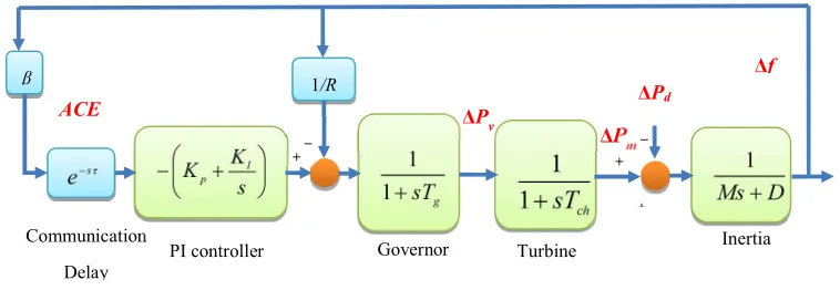
where; g g ch ch c T RT T T M M D A 1 0 1 1 1 0 0 1 g c T B 1 0 0 0 0 1 M
Fc Cc
0 0
T v m
c t f P P
x ( )[ ]
;
ACE t y()
The parameters are defined as: ΔPd is the load deviation, ΔPm is the generator mechanical output deviation, ΔPv is the valve position deviation, Δf is the frequency deviation. M is the moment of inertia, D is the generator damping coefficient, Tg is the time constant of the governor, Tch is the time constant of the turbine, R is the speed drop, and β is the frequency bias factor. For one-area LFC system, the area control error ACE is given as [16]:
f
ACE (2)
Figure 1. Dynamic model of one-area LFC scheme
The AGC has two components; the first is updated every 5 minutes for economical dispatch and the second is updated in the order of 1-5 seconds. The latter signal delay is the one considered in the paper. Stabilizing the system with conventional PI controller given as:
K ACE K ACE
t
u() p I
(3)
where KP is the proportional gain, KI is the integral gain and ∫ ACE is the integration of the
area control error. With the PI controller, the closed-loop system is expressed as follows:
d
dxt F P
A t Ax t
x() () ( ) (4)
where; 0 0 0 0 1 0 1 0 1 1 0 0 0 1
g g
ch ch T RT T T M M D A 0 0 0 0 0 0 0 0 0 0 0 0 0 0 g I g P d T K T K A T M
F 1 0 0 0
T v
m P ACE
P f t
x()[
]The time delay, τ, is composed of transducer delay, analog-to-digital conversion delay, processing delay, multiplexing delay and the delay in the communication link [5]. This time delay
ΔPd
m
P
Δ
β 1/R
v P Δ ACE Δf -+ + -Communication Delay _ _
PI controller Governor Turbine
+
can be constant in dedicated communication links and time varying if open communication is used [16]. Setting ΔPd to zero, the single-area LFC system becomes a linear time delay system, then (4)
becomes:
) ( ) ( )
(t Axt Axt
x d (5)
To find the maximum delay margin, d, we transform (5) using Laplace transform and the
characteristics equation becomes:
0
s
de
A A
sI (6)
Equation (6) is a transcendental equation and have been the subject of the research for many years. The system is asymptotically stable for a given delay if all the roots of (6) lie on the left half plane. The free delay system is assumed to be stable and all the roots are on the left half plane. For some value of the delay one or more roots will cross the imaginary excess. One of the approaches is to replace s with jω and perform the analysis in the frequency domain.
3. Delay Margin Computation Using the Sweeping Test
Time delay systems can be either delay-independent or delay dependent. The delay-dependent system is asymptotically stable for d, marginally stable for d, and unstable for d. The
delay independent system is asymptotically stable for any positive value of the time delay. For the single-area LFC system represented by (5) to be asymptotically stable independent of delay, we must have:
0 ) det( s
de
A A
sI sC, 0 (7)
where Cis the open right half plane. If (7) is satisfied then there are no positive roots for any value of the time delay. The delay dependent stability implies that for time delays less than the delay margin the system is asymptotically stable and all the roots are on the closed left half plane, and when the time delay exceeds the delay margin the system becomes unstable and some roots will be on the right half plane. In this manner, the roots will cross the imaginary axis when d. We are
interested in determining both the delay independent and delay-dependent conditions of the system. To simplify the analysis we replace s by j. Now, we turn our attention to find the delay that produce frequencies on the imaginary axis. Then system (5) is said to be asymptotically stable independent of delay if [23]:
0 ) det( j
de
A A I
j (0,), 0 (8)
If (8) is not satisfied for some values of then the system is delay-dependent stable. Now the problem is to find the crossing frequency, c , where the roots crosses the imaginary axis. To find
the crossing frequencies we use the spectral radius in the following definition.
Definition 1 [24]:
The spectral radius of two matrices pair is defined as:
det( ) 0
min : ) ,
(A Ad AAd
(9)
where i(A)is the ith eigenvalue of the matrix A and i(A,Ad) is the generalized eigenvalue
of matrix pair A, and Ad.
Theorem 1:[24]
For the system (5) stable at τd=0, i.e., A+Ad is stable and rank(Ad)=q, we define
) , 0 ( 1 ) , ( , ] 2 , 0 [ ), , 0 ( ) , ( , min : 1 d i k i k j d i k i i k i k n k i A A I j some for e A A I j if i k
Then d:min1iqi, and the system in (5) is stable for all [0,d) and becomes unstable at
d
. Proof [23-26]:
The system (5) is stable independent of the time delay if the following condition is satisfied:
1 ) , ( ) , ( j d
d j I AAe
A A I
j for 0, 0 (10)
Condition (10) implies that the system is stable with 0, that is, det(AAd)0. Now we
assume that the system becomes unstable for some value of . This means d. Now, we assume that:
0 ) det( j
de
A A I
j (0,) (11)
This can be true for i k
, and consequently at this condition:
1 ) ,
( d
i jI A A
i1,...,n (12) For any [0,d),
i k i
k
we must have:
0 )
det( i
k
j d i
kI A Ae
j (13)
When dthere is a pair ( , ) i k i k
that satisfies i k i k
d
/ , and consequently:
0 ) det(
)
det( i
k d i k j d i k j d i
kI A Ae j I A Ae
j (14) □
Corollary 1 [24]:
The system (5) is stable independent of delay if and only if: (i) A is stable,
(ii) A+Ad is stable, and
(iii) (jIA,Ad)1, 0
The three conditions in Corollary 1 represents the delay independent stability, where (i) states that the system is stable at 0, (ii) the system is stable at and (iii) the system is stable for every in the range [0,).
Theorem 1 determines both the delay independent and the delay dependent stability. First we can verify the delay independent stability by checking the following condition:
1 ) , (jIAAd
(0,)
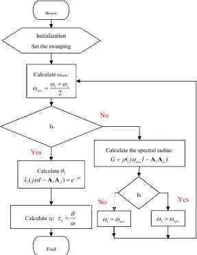
If the above condition is satisfied then the system is stable independent of time delay and if it is not satisfied for some values of ω that makes (jIA,Ad)1 then we calculate the crossing frequencies using the algorithm in Fig. 2. Finally we compute the exact delay margin. The algorithm can be summarized as follows:
Step 1: With the given system parameters, compute A and Ad. Using the sweeping test, check if
the system is stable independent of delay or not, that is (jIA,Ad)1 for (0,). If for some values of , (jIA,Ad)1, then proceed to step 2, otherwise the system is stable independent
of the time delay.
Step 2: Define a range [1,2]. At 1 the spectral radius (jIA,Ad)1 and at 2 the
spectral radius (jIA,Ad)1. Now the crossing frequency, c, lies in the range from 1 to 2
Step 3: Use the binary iteration to find the crossing frequency, c, with a given error tolerance
e
[27, 28]. We set new(12)/2 , if (jnewIA,Ad)1 then 2 new and if
1 ) , (jnewIAAd
then 1 new. Now the search range is reduced every iteration until the desired
accuracy is reached.
Step 4: When the desired accuracy is reached we calculate i k
, the crossing angles, through
solving i
k
j d i k
i j I A A e
( , ) . Finally, i
k i k n k
d
min /
1
is the desired delay margin.
4. Case Study: One-Area LFC system
To compare the results of our proposed method with the published ones we use the same parameters in [16,18,22]. The parameters of the LFC system shown in Fig. 1 are given as: Tch=0.3,
Tg=0.1, R=0.05, D=1.0, β=21.0 and M=10. Under open communication network the remote terminal
unit (RTU) sends the signals to the central controller through the shared network, and then the controller sends the commands back. In most of the studies these two delays are aggregated into a single delay and this assumption is made in this paper. The ACE signals are updates every 2-4 s [10]. In power systems the data collection is in the order of 1−5 s [4]. The results of the delay margin with different values of the controller gains, KP and KI are shown in Table 1 along with the results of the
methods in [16,18,22]. It should be noted that the method in [22] gives the most accurate reported delay margins. Table 1 shows clearly that the proposed method gives almost exactly as the results of the method reported in [22], however, the proposed method is simpler with less computations.
Figure 2. The delay margin calculation algorithm
Initialization Set the sweeping
Calculate the spectral radius:
Is Is
End
Calculate θ:
Calculate τd:
Calculate ωnew:
Start
Yes
No
The delay margin as function of the integral gain for various values of the proportional gain with the proposed method and the method reported in [22] are shown in Figs 3-9. As can be seen the proposed method accurately determines the delay margin for the single-area LFC system. The relative error between the proposed method and the method published in [22] is very small. The average relative percentage error is 0.023867% which shows that the delay margin values are nearly exactly as the same reported in [22].
Table 1. The delaymargin for different values of KP and KI
τd, s KI
KP Method 0.05 0.1 0.15 0.2 0.4 0.6 1.0
0 Theorem.1 [22] [18] [16] 30.928 30.915 30.853 27.927 15.207 15.201 15.172 13.778 9.961 9.960 9.942 9.056 7.338 7.335 7.323 6.692 3.382 3.382 3.377 3.124 2.042 2.042 2.040 1.910 0.923 0.923 0.922 0.886 .05 Theorem.1
[22] [18] [16] 31.851 31.875 31.498 27.874 15.687 15.681 15.647 14.061 10.277 10.279 10.258 9.284 7.573 7.575 7.561 6.866 3.502 3.501 3.496 3.215 2.122 2.122 2.119 1.974 0.970 0.970 0.969 0.927 0.1 Theorem.1
[22] [18] [16] 32.769 32.751 30.415 27.038 16.127 16.119 15.765 13.682 10.575 10.571 10.547 9.220 7.793 7.794 7.777 6.941 3.610 3.610 3.604 3.290 2.194 2.194 2.191 2.029 1.012 1.012 1.011 0.963 0.2 Theorem.1
[22] [18] [16] 34.198 34.226 28.010 25.114 16.860 16.856 14.597 12.760 11.060 11.062 10.107 8.617 8.160 8.162 7.821 6.535 3.792 3.792 3.784 3.320 2.313 2.313 2.309 2.108 1.079 1.079 1.077 1.016 0.4 Theorem.1
[22] [18] [16] 35.802 35.834 22.457 20.364 17.661 17.658 11.835 10.426 11.596 11.594 8.287 7.065 8.559 8.559 6.505 5.384 3.981 3.980 3.718 2.832 2.426 2.426 2.419 1.912 1.118 1.118 1.116 1.017 0.6 Theorem.1
[22] [18] [16] 34.906 34.922 16.033 14.618 17.198 17.195 8.624 7.477 11.280 11.278 6.209 5.157 8.311 8.312 4.997 3.958 3.826 3.826 3.038 2.130 2.281 2.281 2.178 1.475 0.947 0.947 0.964 0.827 1.0 Theorem.1
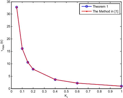
Figure 3. The delay margin as function of the integral gain, KI with KP=0
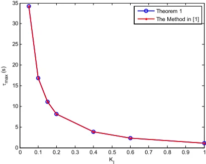
Figure 4. The delay margin as function of the integral gain, KI with KP=0.05
Figure 5. The delay margin as function of the integral gain, KI with KP=0.1
0 0.1 0.2 0.3 0.4 0.5 0.6 0.7 0.8 0.9 1
0 5 10 15 20 25 30 35
KI
max
(
s)
Theorem 1 The Method in [1]
0 0.1 0.2 0.3 0.4 0.5 0.6 0.7 0.8 0.9 1
0 5 10 15 20 25 30 35
KI
max
(
s)
Theorem 1 The Method in [1]
0 0.1 0.2 0.3 0.4 0.5 0.6 0.7 0.8 0.9 1
0 5 10 15 20 25 30 35
KI
ma
x
(
s)
Figure 6. The delay margin as function of the integral gain, KI with KP=0.2
Figure 7. The delay margin as function of the integral gain, KI with KP=0.4
Figure 8. The delay margin as function of the integral gain, KI with KP=0.6
0 0.1 0.2 0.3 0.4 0.5 0.6 0.7 0.8 0.9 1
0 5 10 15 20 25 30 35
KI
max
(
s)
Theorem 1 The Method in [1]
0 0.1 0.2 0.3 0.4 0.5 0.6 0.7 0.8 0.9 1
0 5 10 15 20 25 30 35 40
KI
max
(
s)
Theorem 1 The Method in [1]
0 0.1 0.2 0.3 0.4 0.5 0.6 0.7 0.8 0.9 1
0 5 10 15 20 25 30 35
KI
ma
x
(
s)
Figure 9. The delay margin as function of the integral gain, KI with KP=1.0
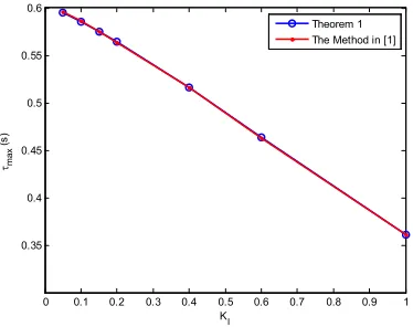
Case I (KP=0 and KI=0.4): In [22] it is reported that the delay margin with KP=0 and KI=0.4 is 3.382
s, with the proposed method it is 3.382 s. The proposed method gives accurate values of the delay margin as the method reported in [22]. The proposed method give less conservative results than the LMI methods reported in [16,18]. To validate the results, simulations with Matlab/Simulink are carried out. The frequency response of the LFC system with KP=0 and KI=0.4 for different values of
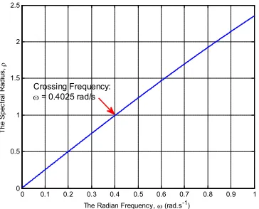
the time delay is shown in Fig. 10. A 0.1 p.u change in the load occurs at 10 s. Fig. 10 shows the frequency response with 3.3 s, 3.382 s and 3.4 s, and it is clear that the system is stable with 3.3 s and unstable with 3.4 s. From the simulation the system is marginally stable with 3.384 s. The percentage error with the simulation based delay margin is 0.071%. For this system we have only one generalized eigenvalue. The spectral radius as function of ω is shown in Fig. 11. From Fig. 11 the crossing frequency is 0.4025 rad/s, solving (14), we have θ = 1.3678 rad which makes the delay margin equals 3.382 s. From Fig. 10 the oscillating frequency is 0.4025 rad/s which proves the validity of the results.
Figure 10. The frequency response for different values of the time delay with KP=0 and KI=0.4
0 0.1 0.2 0.3 0.4 0.5 0.6 0.7 0.8 0.9 1
0.35 0.4 0.45 0.5 0.55 0.6
KI max
(
s)
Theorem 1 The Method in [1]
0 10 20 30 40 50 60 70 80 90 100
-8 -6 -4 -2 0 2 4 6 8
10x 10
-3
Time, (seconds)
F
re
qu
en
cy
D
ev
ia
tio
n,
f,
(p
.u
)
= 3.300 s
=3.382
Figure 11. The spectral radius as function of ω for KP=0 and KI=0.4
Case II (KP=0.6 and KI=0.6): In [22] it is reported with KP=0.6 and KI=0.6 that the delay margin is
2.281 s, while with our method it is 2.281 s. The frequency response with different delays is shown in Fig. 12. The system is stable with 2.1 s, however it becomes unstable with 2.4 s which is larger than the delay margin. The simulation based delay margin is 2.282 s. The crossing frequency is 0.8015 rad/s , solving (14) for θ then; θ = 1.8283 rad. Fig. 13 shows the spectral radius as function of ω for KP=0.6 and KI=0.6.
Case III (KP=0.05 and KI=0.05): In [22] it is reported with KP=0.05,KI=0.05 that the delay margin is
31.875 s, while with our method it is 31.8509 s. The frequency response with different delays is shown in Fig. 14. The system is stable with 31.8509 s, however it becomes unstable with 33 s which is larger than the delay margin. The simulation based delay margin is 31.88 s. The relative percentage error is 0.0438%. The crossing frequency is0.0502 rad/s , solving (14) for θ then θ = 1.596 rad. Fig. 15 shows the spectral radius as function of ω for KP=0.05 and KI=0.05.
Figure 12. The frequency response for different values of the time delay with KP=0.6 and KI=0.6
0 0.1 0.2 0.3 0.4 0.5 0.6 0.7 0.8 0.9 1
0 0.5 1 1.5 2 2.5
T
he
S
pe
ct
ra
l R
ad
iu
s,
The Radian Frequency, (rad.s-1) Crossing Frequency:
= 0.4025 rad/s
0 10 20 30 40 50 60 70 80 90 100
-0.015 -0.01 -0.005 0 0.005 0.01 0.015
Time, (seconds)
F
re
qu
en
cy
D
ev
ia
tio
n,
f,
(p
.u
)
= 2.100 s
= 2.281 s
Figure 13. The spectral radius as function of ω for KP=0.6 and KI=0.6
Figure 14. The frequency response for different values of the time delay with KP=0.05 and KI=0.05 The delay margin for different values of the PI controller gains is shown in Fig. 16. The delay
margin dependence on KI, and KP showed similar behavior as in [16,18,22]. Additionally, the crossing
frequencies and crossing angles are shown in Table 2 and 3 respectively. The variation of the crossing angle and the crossing frequency gives more details on the dependence of the delay margin on KP
and KI. From Fig. 16 the delay margin decreases with increasing KI if KP is kept constant. The delay
margin increases as KP increase in the range KP<0.4, then the delay decreases as KP becomes larger
than 0.4. This is the same behavior observed in [16,18,22]. The delay margin becomes large for small values of KP and KI.
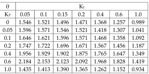
Table 2. The crossing angle with different values of KP and KI
θ KI
KP 0.05 0.1 0.15 0.2 0.4 0.6 1.0
0 1.546 1.521 1.496 1.471 1.368 1.257 0.989 0.05 1.596 1.571 1.546 1.521 1.418 1.307 1.041 0.1 1.646 1.621 1.596 1.571 1.468 1.358 1.092 0.2 1.747 1.722 1.696 1.671 1.567 1.456 1.187 0.4 1.956 1.929 1.902 1.875 1.765 1.647 1.349 0.6 2.184 2.153 2.123 2.092 1.968 1.828 1.419 1.0 1.435 1.413 1.390 1.365 1.262 1.152 0.934
From Table 3, the LFC system oscillate with lower frequencies for small values of KP and KI. The
LFC system tends to oscillate with higher frequency with large values of KP and KI.
0 0.1 0.2 0.3 0.4 0.5 0.6 0.7 0.8 0.9 1 0
0.2 0.4 0.6 0.8 1 1.2 1.4
The Radian Frequency, (rad.s-1)
T
he
S
pe
ct
ra
l R
ad
iu
s,
Crossing Frequency:
= 0.8015 rad/s
0 50 100 150 200 250 300 350 400 450 500
-8 -6 -4 -2 0 2 4 6 8x 10
-3
Time, (seconds)
F
re
qu
en
cy
D
ev
ia
tio
n,
f,
(p
.u
)
= 31.0000 s
= 31.8509 s
Figure 15. The spectral radius as function of ω for KP=0.05 and KI=0.05
Figure 16. The delay margin with different values of KP and KI
Table 3. The crossing frequency with different values of KP and KI
Ω KI
KP 0.05 0.1 0.15 0.2 0.4 0.6 1.0
0 0.0500 0.1000 0.1502 0.2005 0.4045 0.6153 1.0714 0.05 0.0501 0.1002 0.1505 0.2009 0.4050 0.6161 1.0732 0.1 0.0502 0.1005 0.1509 0.2016 0.4067 0.6187 1.0784 0.2 0.0511 0.1021 0.1534 0.2048 0.4133 0.6295 1.1004 0.4 0.0546 0.1092 0.1640 0.2191 0.4434 0.6789 1.2065 0.6 0.0626 0.1252 0.1882 0.2518 0.5143 0.8015 1.4981 1.0 2.4102 2.4120 2.4151 2.4193 2.4462 2.4861 2.5867
The delay margins, crossing angles and the crossing frequencies with different values of KI when
KP=0 are shown in Table 4. It is interesting to observe that the crossing frequency with KP=0
numerically equals KI. As KP is made larger than 0.2, the crossing frequency increases with increasing
KP
Table 4. The delay margin for various values of KI and KP=0
KI θ ω τd
0.05 1.5460 0.0500 30.9283 0.1 1.5212 0.1000 15.2066 0.15 1.4963 0.1502 9.9614
0.2 1.4712 0.2005 7.3375 0.4 1.3678 0.4045 3.3816 0.6 1.2566 0.6153 2.0422 1.0 0.9889 1.0714 0.9230
0 0.01 0.02 0.03 0.04 0.05 0.06 0.07 0.08 0.09 0.1 0
0.2 0.4 0.6 0.8 1 1.2 1.4 1.6 1.8 2
The Radian Frequency, (rad.s-1)
T
he
S
pe
ct
ra
l R
ad
iu
s,
Crossing Frequency: = 0.0501 rad/s
0 0.5
1 1.5
0 0.2 0.4 0.6 0.8 1 0 10 20 30 40
KI KP
ma
The proposed method has been compared with four different published methods. The delay margin results are less conservative than the results of the LMI method reported in [16,18], however, the LMI method which are time domain methods have an advantage of dealing with time varying delays. The results of the delay margin are equal to the delay margins obtained by the frequency domain methods reported in [20,22], however, the proposed method is simpler for implementation.
5. Conclusions
In this paper we propose a method for analyzing the stability of load frequency control system with communication delay. The method is a frequency domain method without any approximation to the resultant delay system. The delay margins are computed through the binary iteration and the sweeping test. A single-area load frequency control system has been chosen as case study and the delay margin values have been compared with values reported in the literature. The method gives accurate delay margin which is proved by time delay simulation and comparison with the published methods. The main two advantages of the proposed method is its accuracy and simplicity compared with the other methods. Additionally, the method can determine accurately the oscillating frequency of the load frequency control system when the time delay equals the delay margin. The proposed method in this paper is applied to single delay load frequency system. The method will be extended to deal with multiple time delays which is the case for multi-area load frequency control system.
References
1. H. Saadat, Power System Analysis, New York: McGraw-Hill Companies, 1999.
2. S. Bhowmik, K. Tomsovic, and A. Bose, "Communication Models for Third Party Load Frequency Control
," IEEE Transactions on Power Systems, vol. 19, no. 1. pp.543-548, 2004.
3. A . Khalil, J. Wang, and O. Mohammed, "Robust stabilization of load frequency control system under
networked environment," International Journal of Automation and Computing, vol. 14, no. 1. pp.93-105, 2017.
4. K. H. Mak and B. L. Holland, "Migrating electricalpower network SCADA systems to TCP/IP and Ethernet
networking," Power Engineering Journal, vol. 16, no. 6. pp.305-311, 2002.
5. B. Naduvathuparambil, M. C. Valenti, and A. Feliachi, "Communication delays in wide area measurement
systems." Proceedings of the Thirty-Fourth Southeastern Symposium on System Theory , pp. 118-122. 2002 .
6. H. Bevrani and T. Hiyama, "A control strategy for LFC design with communication delays." 2005
International Power Engineering Conference , pp. 1087-1092. Nov. 2005 .
7. Y. Xiaofeng and K. Tomsovic, "Application of linear matrix inequalitiesfor load frequency control with
communication delays," IEEE Transactions on Power Systems, vol. 19, no. 3. pp.1508-1515, Aug., 2004.
8. C. K. Zhang, L. Jiang, Q. H. Wu et al., "Delay-Dependent Robust Load Frequency Control for Time Delay
Power Systems ",IEEE Transactions on Power Systems, vol. 28, no. 3. pp.2192-2201, Aug., 2013.
9. C. Peng and J. Zhang, "Delay-Distribution-Dependent Load Frequency Control of Power Systems With
Probabilistic Interval Delays," IEEE Transactions on Power Systems, vol. 31 ,no. 4. pp.3309-3317, 2016.
10. C. K. Zhang, L. Jiang, Q. H. Wu et al., "Further Results on Delay-Dependent Stability of Multi-Area Load
Frequency Control," IEEE Transactions on Power Systems, vol. 28, no. 4. pp.4465-4474, Nov., 2013.
11. Rajeeb Dey, Sandip Ghosh, G. Ray et al., "H1 load frequency control of interconnected power systems with
communication delays," Electrical Power and Energy Systems, vol. 42, no. 2012. pp.672-684, 2012.
12. Pegah Ojaghi and Mehdi Rahmani, "LMI-Based Robust Predictive Load Frequency Control for Power
Systems With Communication Delays," IEEE Transactions on Power Systems, vol. 32, no. 5. pp.4091-4100, 2017.
13. Vijay P. Singh, Nand Kishor, and Paulson Samuel, "Load Frequency Control with Communication
Topology Changes inSmart Grid," IEEE Transactions on Industrial Informatics, vol. 12, no. 5. pp.1943-1952, 2016.
14. H. Bevrani and T. Hiyama, "On Load Frequency Regulation With Time Delays: Design and Real-Time
15. A. Khalil and J. Wang, "Stabilization of load frequency control system under networked environment."
Automation and Computing (ICAC), 2015 21st International Conference on, pp. 1-6. Sept. 2015 .
16. L. Jiang, W. Yao, Q. H. Wu et al., "Delay-Dependent Stability for Load Frequency Control With Constant
and Time-Varying Delays," IEEE Transactions on Power Systems, vol. 27, no. 2. pp.932-941, May, 2012.
17. Y. He, J.-H. She, and M. Wu, Stability Analysis and Robust Control of Time-Delay Systems: Springer, 2010.
18. K. Ramakrishnan, "Delay-dependent stability criterion for delayed load frequency control systems2016 ".
IEEE Annual India Conference (INDICON) , pp. 1-6. 2016 .
19. K. Ramakrishnan and G. Ray, "Improved results on delay dependent stability of LFC systems with multiple
time delays," Journal of Control, Automation and Electrical Systems, vol. 2015, no. 26. pp.235-240, 2015.
20. S. Sonmez, .Ayasun, and U. Eminoglu, "Computation of time delay margins for stability of a single-area
load frequency control system with communication delays.," WSEAS TRANSACTIONS on POWER SYSTEMS ,vol. 9, no. 2014. pp.67-76, 2014.
21. Sahin Sonmez and SAFFET AYASUN, "Stability Region in the Parameter Space of PI Controller for a
Single-Area Load Frequency Control System With Time Delay," IEEE Transactions on Power Systems, vol. 31, no. 1. pp.829 ,830-Jan., 2016.
22. Sahin Sonmez, SAFFET AYASUN, and Chika O. Nwankpa, "An Exact Method for Computing Delay
Margin for Stability of Load Frequency Control Systems With Constant Communication Delays," IEEE Transactions on Power Systems, vol. 31, no. 1. pp.370-377, Jan., 2016.
23. Jie Chen, "On Computing the Maximal Delay Intervals for Stability of Linear Delay Systems," IEEE Transactions on Automatic Control, vol. 40, no. 6. pp.1087-1093, 1995.
24. Keqin Gu, Vladimir L. Kharitonov, and Jie Chen, Stability of Time-Delay Systems: Springer, 2003.
25. Jie Chen and Haniph A. Latchman, "Frequency Sweeping Tests for Stability Independent of Delay," IEEE
Transactions on Automatic Control, vol. 40, no. 9. pp.1640-1645, 1995.
26. Jie Chen, Guoxiang Gu, and CarlN. Nett, "A New Method for Computing Delay Margins for Stability of
Linear Delay Systems." IEEE 33rd Conference on Decision and Control , pp. 433-437. 1994. Lake Buena Vista, FL .
27. S. Elkawafi, A. Khalil, A. I. Elgaiyaret al., "Delay-dependent stability of LFC in Microgrid with varying time delays." 2016 22nd International Conference on Automation and Computing (ICAC). pp. 354-359. 2016. Colchester, UK .