Model-based systems engineering with requirements variability for embedded real-time systems

Model-Based Systems Engineering with

Requirements Variability for Embedded Real-Time

Systems

Mole Li, Firat Batmaz, Lin Guan

Loughborough, UK [email protected]

Alan Grigg, Matthew Ingham

Services Derby, UK

[email protected]

Peter Bull

Birmingham City University Birmingham, UK [email protected]

Abstract—Product Line Engineering (PLE) offers the benefits of reducing costs and time to market by reusing requirements and components. Current PLE methods, however, mainly focus on the software aspects and are lacking in support for many system level concerns like physical and non-functional require-ments (Quality of Service attributes) that play an important role in the development of Embedded Real-Time Systems (RTS). This paper proposes a new method to support a combination of variability modelling (a key feature of PLE) and model-based requirement engineering (in SysML) for Embedded RTS. It provides four main contributions: 1. it extends the Orthogonal Variability Model (OVM) to support the separation of function-al, physical and non-functional variability; 2. it proposes a mechanism for the evolution of variability; 3. stakeholders’ specifications for variable requirements are extended by the proposed approach; 4. it increases the consistency of system models by directly using SysML Activity Diagrams and Block Definition Diagrams as a base model for refining variability models for requirement representation. The proposed method is illustrated by an Aircraft Engine Control System case study.

Index Terms—Product Line, Requirement Engineering, Embedded Real-Time System, Variability Modelling.

I.INTRODUCTION

To meet the requirements of competitive pressures, Em-bedded Real-Time Systems (RTS) need to leverage advanced technology to offer a capability that can reduce development costs and shorten development times. Traditionally, Model-Based System Engineering (MBSE) uses modelling languages such as Unified Modelling Language (UML) and Systems Modelling Language (SysML) to meet these demands by de-termining the system requirements and foreseeing the risks at an early stage [1].

Nowadays, fewer industrial projects start to develop sys-tems from scratch. Today’s syssys-tems development rather tends to use and upgrade existing designs to produce new products [2]. For coping with demand, Product Line Engineering (PLE) has drawn a great deal of attention, as it improves time to market, cost, quality and productivity by identifying common-alities and variabilities between existing systems to provide reusability [3]. As P. Clements and L. Northrop [3] mentioned,

PLE is managed by a requirement engineering-change man-agement process. The key feature of PLE is variability model-ling [4]. This distinguishes PLE from traditional System Engi-neering approaches by explicitly considering system diversity, including requirement diversity, for reusability purposes. It refers to the ability of systems requirements to be configured, customised and extended for specific contexts [5]. Due to the importance of variability modelling in PLE, a great number of researchers focus on addressing the challenges that come with it. The earliest variability method, Feature-Oriented Domain Analysis (FODA) [6], can be traced back to the 1990s. In the years between 1990 and 2014, several variability modelling methods and systematic literature reviews [7-11] were pub-lished, taking into account different contexts, aspects, devel-opment stages and purposes. Specifically, the systematic liter-ature review paper by V. Alves, N. Niu, C. Alves and G. Valença [10] focused on requirement engineering for Software Product Line. However, many Product Line Engineering pub-lications on System Engineering are actually focussed on only the software aspect [12]. While Software Product Line Engi-neering is important in the systems domain, System Engineer-ing is a much broader discipline; it includes the consideration of hardware aspects (mechanical and electrical engineering) as well as the overall integration of hardware and software com-ponents [13].

Therefore the aim of this paper is to propose a practical variability modelling method that can be combined with mod-el-based requirement engineering in the Embedded RTS do-main. To fulfil this aim, the proposed requirement variability model should represent and separate functional, physical and non-functional requirements clearly.

The rest of the paper is structured as follows: Section II provides information on fundamental concepts of Product Line Engineering, summarises related works and traditional requirement modelling approaches for the Embedded RTS (without reusability concerns); Section III introduces the pro-posed modelling approach; Section IV provides a case study of an Aircraft Engine Control System to further explain the proposed method and the applied modelling tool; Section V discusses the contributions of the proposed method and the differences between it and related works. Finally, a conclusion to this paper and information about future work are provided.

II.BACKGROUND AND RELATED WORKS

This section gives an introduction on Product Line Engi-neering and variability modelling classification. This is fol-lowed by the introduction of traditional Embedded RTS re-quirement modelling methods. Numerous methods exist for model-based requirement engineering for Embedded RTS and variability modelling. This section briefly introduces related works by classification group.

A. Classification of Variability Modelling Methods

As previously mentioned, variability modelling is the key feature of PLE. It defines how the system requirements of a product line asset can vary [17]. This paper adopts A. Metzger and K. Pohl’s classification [9]: “integrated variability docu-mentation” and “orthogonal variability docudocu-mentation”.

“Integrated variability documentation” refers to the mod-elling methods that represent the commonalities and variabili-ties of systems together in the same model. For example, the feature model [6] illustrates common and variable features (via an optional feature) of a system on a feature diagram. As S. Sepúlveda, C. Cares and C. Cachero [18] stated, feature modelling is the most common method of variability model-ling in Software Engineering. It is a tree-like structure which represents both the commonality and variability features of products in a product line. Each feature model consists of a root that is the software product family, and leaves that are the components that can be selected [19].

“Orthogonal variability documentation” involves the sepa-ration of commonalities and variabilities into different dia-grams. Variability is treated as the first class and based on the concept of the variant and the variation point. The variation point describes where variability occurs. A variant is an in-stance of a variable item [20]. In addition, orthogonal variabil-ity documentation only handles variants on its diagram, and is linked with commonality models or artefacts. It has attracted a lot of attention in recent publications [12] [21], because it does not require changing the complexity of development artefacts and can be combined with different development artefacts [20]. For this classification, most recent efforts, such as the

Orthog-onal Variability Modelling (OVM) [22] (which was adopted as ISO/IEC standard #26550 in 2013) are examples. It repre-sents variability in terms of variation points and variants. The variation points and variants can be linked to a base model specified by UML or SysML. Common Variability Language (CVL) [23] is an Object Management Group (OMG) standard proposal for variability modelling. It consists of a user-centric layer and a product realisation layer. The user-centric layer is used for high-level variability representation in terms of the feature model. The realisation layer defines lower level opera-tions for transformation from the base model to a new, solved model [23]. It specifies how an individual feature is imple-mented on the base model.

B. Integrated Variability Documentation

A number of works consider feature modelling with the variability of non-functional requirements. For example, E. Bagheri, M. Asadi, D. Gasevic and S. Soltani [28] extend feature models with the meta-class to represent non-functional requirements. L. Etxeberria and G. Sagardui [29] create a quality feature tree in a feature model to represent non-functional requirements. Another paper by L. Belategi, G. Sagardui and L. Etxeberria [30] also uses a quality feature tree to model non-functional requirements and a MARTE profile for platform resource representation. In addition, MARTE is also utilised for quality analysis in the design stage.

There is another trend in integrated variability documenta-tion, which is extending UML or SysML by stereotypes to support variability representation. For instance, AspectSM [31] extends the UML State Machine Diagram and Class Diagram with stereotypes for variability modelling. It organises these models in two packages: the software package contains the State Machine Diagram to model the core behaviours and functional behaviours; the hardware package contains the Class Diagram for representing hardware configurations. Non-functional behaviours are modelled as class attributes via MARTE.

Some approaches merge feature models with UML or SysML. Feature models are used for the high-level abstraction of variability, and then UML or SysML is used for refinement. S. Trujillo et al. [32] proposed combining the feature model with extended SysML (by stereotypes for variability model-ling). The feature model handles high-level requirements. Structural and behavioural variability is handled by variation point notation.

In practice, industrial projects often start with legacy sys-tems and software requirements. As the paper by C. Dumitres-cu et al. [33] suggests, variability should be compatible with legacy documents. Using the integrated variability documenta-tion method requires changing the complexity of development artefacts by introducing both commonality and variability into existing models [9].

C. Orthogonal Variability Documentation

Diagram to model the structural design and safety require-ments. Functional requirement variability is represented in the user-centric layer as a feature model. Similarly, P. Queiroz and R. Braga [35] also use CVL with SysML and MARTE. For requirement variability modelling, it utilises a SysML Requirement Diagram with a CVL feature in the user-centric layer. However, it takes on the disadvantages of integrated variability documentation, and in particular the fact that the CVL’s user-centric layer is a feature model.

Unlike CVL, OVM only models variability in parts. Some researchers have implemented OVM with SysML in industrial settings [36] [12] [37]. While OVM allows variation points and variants to link with base models (SysML) to illustrate the variability of different requirement types, such as functional, physical and non-functional requirements. However, it is hard to identify whether a variability requirement is functional, non-functional or physical if it is only based on a variability model of OVM.

D. Requirement Modelling for Embedded Real-Time Sys-tems

According to S. Friedenthal, A. Moore and R. Steiner [1], conventionally engineers model system requirements using SysML Requirement Diagrams, which are graphical represen-tations of textual system requirements. SysML Activity Dia-grams, which show sequences of the elementary actions of systems, are then generated to model system behaviours. A SysML Block Definition Diagram can be used to represent hardware architecture.

As M. Rashid, M. W. Anwar and A. M. Khan [24] men-tion, requirement modelling is the most important activity for Embedded Real-Time System Engineering, so requirements are modelled with different verification and validation con-cerns. Some approaches [25] [26] have been proposed to mod-el system requirements with SysML Activity Diagrams to facilitate the verification of requirements. For example, E. Andrade, P. Maciel, G. Callou and B. Nogueira [26] use the Activity Diagram in SysML and combine it with the Model-ling and Analysis of Real-Time and Embedded Systems (MARTE) to verify the functional, timing and low-power re-quirements of the embedded system. MARTE [27] is a UML profile which is used for the modelling and verification of non-functional requirements of Embedded RTS. Activity Dia-grams are used for requirement modelling by E. Andrade, P. Maciel, G. Callou and B. Nogueira [26]. MARTE is used for timing and energy value representation with stereotypes of best-case and worst-case response times. The Activity Dia-gram, with quantitative data, is then translated into a Time Petri Net with Energy constraints (ETPN) for non-functional property estimation.

In summary, integrated variability documentation requires more effort than orthogonal variability documentation when being adopted for large scale industries that apply re-use of numerous legacy requirements. The reason for this is that in-tegrated variability documentation requires changing existing models to express both commonality and variability. For exist-ing orthogonal variability methods, there are also some

chal-lenges which need to be solved to enable modelling require-ment variability in Embedded RTS:

V. Alves, N. Niu, C. Alves and G. Valença [10] sug-gest that requirement engineering with PLE should consider multiple stakeholder aspects including those of customers, systems engineers, software engineers and hardware engineers. However, current orthogonal variability methods cannot illustrate which stakehold-er is responsible for a cstakehold-ertain variation point or variant. According to L. Chen, L and M. A. Babar [38], who investigated the industrial challenges of PLE, variabil-ity of requirements exists not only in space ences between systems) but also over time (differ-ences between times). Current orthogonal variability methods do not support the specification of the evolu-tion of variability.

Most requirement variability modelling is based on UML Use Case Diagrams or SysML Requirement Di-agrams. As stated above, using SysML Activity Dia-grams for requirement modelling in Embedded RTS facilitates requirement verification and validation. Therefore modelling requirement variability for Em-bedded RTS using SysML Activity Diagram is more beneficial when it comes to verification and validation. However, current requirement modelling methods that use SysML Activity Diagrams do not support consid-eration of the variability aspect.

III.PROPOSED APPROACH

This section introduces the proposed method for modelling requirement variability for Embedded RTS. To cope with the challenges mentioned above, this proposed method adopts OVM as its core variability modelling means, and extends it to support representations of variability types, stakeholders and the evolution of variability. Adopting OVM also leads to a model that is less complex than integrated variability docu-mentation methods [9]. This approach also integrates the pro-posed variability model with SysML in order to support re-quirement engineering with a variability aspect in the Embed-ded RTS domain.

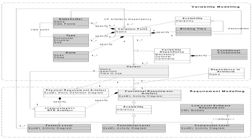
Figure 1. The meta-model of the Embedded RTS requirement variability modelling approach

time and stakeholders. The requirement modelling part shows the commonality and variability of system requirements through SysML Activity Diagrams and Block Definition Dia-grams. The existing legacy system requirement models are not changed. The variable requirements are introduced by adding variable artefacts (refinements of each variant) to existing models. The definitions and semantics of each concept of the meta-model are introduced as follows:

A. Variability Modelling

“Variation point” has the same meaning as in OVM, i.e. describes where variability occurs. However, the proposed method extends it with stakeholder, state, type and binding time information. This is the starting point for building a variability model. The functional variation point can be linked or refined using a Fea-ture Level requirement diagram (SysML Activity Di-agram). This proposal adopts the concept of state in [49]. The “state” of the variation point indicates whether the variation point can be modified to accept new variants during future development. Normally the state “Open” is used to show that the variation point is modifiable. In contrast, “Close” means the variation point cannot be changed.

“Stakeholder” is a tag that works on a variation point to identify the people who are responsible for this var-iation point. For example, domain experts may man-age functional variation points. Customers may

inter-act with physical resource variation points, especially on system level interfaces.

“Type” is a tag for the variation points, which repre-sents whether it is related to functional, physical or Quality of Service (QoS) attributes (non-functional). Variants are of the same type as their linked variation points.

“Binding time” is a tag that indicates when a certain variation point should be instantiated. It is important to specify when to bind a specific variant to its varia-tion point [47]. A typical binding time might be “Do-main Requirement Stage”, which means “determine the variation point when considering requirement commonality and variability”, or “Application Re-quirement Stage”, which means “decisions on the var-iation points are made when specific customers’ re-quirements arrive”.

“Scalability” refers to a hierarchy representation in the structure to reduce the complexity of diagrams. As re-ported, there are hundreds or even thousands of com-mon and variable models in real industry situations [38] [40]. It is impossible to represent all this infor-mation in one diagram. Therefore, modelling require-ments or variability in a hierarchical manner reduces the complexity of requirement and variability dia-grams and satisfies real industrial needs.

Figure 2. The Gas Turbine Engine [51]

over time. In order to represent this information, the proposed approach uses “Time in Use” to describe the valid period of the variant. In addition, the variant can link with different requirement artefacts for further re-finement, such as SysML Activity Diagrams and Block Definition Diagrams, via “Dependency on Ar-tefacts”.

Dependency between variation points and variants is mainly kept the same as in OVM, except for the con-ditional constraints extension. Sometimes, the variant exists only in certain conditions or context [48]. “Conditional constraints” illustrate a suitable situation that instigates the variant for the linked variation point. For example, the variant “Reliable Sensor” should be selected when the Conditional Constraint is et >£10000”. “Dependency to Artefacts” is used to link requirement artefacts to variants.

B. Requirement Modelling

“Functional Requirement Artefacts” refer to the SysML Activity Diagram to represent functional re-quirements. Unlike the traditional SysML model, which uses Requirement Diagrams for requirement specifications, the proposed method uses Activity Di-agrams in a hierarchical structure. Each activity in the Activity Diagram represents either a functional re-quirement or a group of rere-quirements at the “Func-tional Level”. The “Feature Level” is a higher-level abstraction and it is used to group functions to facili-tate the reuse of requirements. “Component Level” requirements can be transformed into “Low-Level Software Requirements” for the software team. This approach has been developed by the Rolls-Royce Control and Data Services team who are supporting the current research. The details of this are beyond the scope of this paper. The reason for using Activity Di-agrams instead of Requirement DiDi-agrams for func-tional requirement specification is twofold: firstly, it increases the consistency of system models and allows functional requirements to be refined into system be-haviours through a “parent to child” relationship (hi-erarchy) in the Activity Diagram; secondly, require-ment verification methods that are based on Activity Diagrams can then be used when an individual prod-uct is to be generated from the prodprod-uct line [25] [26]. The “Physical Requirement Artefact” uses a SysML Block Definition Diagram to represent physical re-quirements. The Block Definition Diagram also al-lows the representation of a physical resource struc-ture.

The “NFR Artefact” refers to the representation of non-functional requirements in terms of stereotypes. These stereotypes are implied on the Activity Dia-gram and Block Definition DiaDia-gram to show the non-functional requirements and their relationships with functional and physical requirements. The addition of quality attributes also provides a starting point for

per-forming automated non-functional analysis on the sys-tem model. However, quality attributes analysis is be-yond the scope of this paper.

IV.CASE STUDY

This section introduces a case study of an Engine Control System to demonstrate the proposed approach. Initially, a tex-tual description of Engine Control System requirements, in-cluding commonalities and variabilities is given. Then our proposed model for Engine Control System requirements en-gineering is introduced.

A. Engine Control System

A simplified gas turbine engine is introduced by I. Habli, T. Kelly and I. Hopkins [41]. As Figure 2 shows, it has a fan and a compressor to absorb a large volume of air. The air is mixed with fuel and ignited in a combustion chamber. Prior to com-bustion, the air is compressed to up to 40 times atmospheric pressure. After combustion, the combustion exhaust gases are forced (expand) through a turbine to provide thrust.

According to L. C. Jaw and J.D. Mattingly [42], the Full Authority Digital Electronic Controls System (FADEC) has become the standard engine control system for modern gas turbine engines. FADEC helps pilots to monitor and control engine parameters and warns them when abnormal conditions occur.

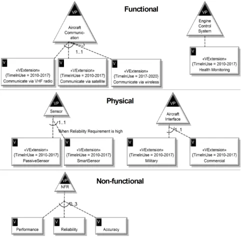
Control-Figure 3. Variability model of Engine Control System

Figure 4. Variation Point <<VPExtension>> stereotype

ler and Engine Databus. The variable physical resources re-quirement is “inlet air temperature (T1) and pressure (P1), which use passive or smart sensors”. The difference is that smart sensors increase the reliability of T1 and P1 measure-ments. In addition, smart sensors simplify wiring and reduce weight, as they can communicate with the Electronic Engine Control via the Engine Databus. The other variable physical resource requirement is Aircraft Interface.

B. Variability Model of Engine Control System

The initial step for requirement variability modelling is generating the variability model. This is shown in Figures 3 and 4. This model only represents the variability of the system requirements. The common requirements are modelled by a base model (SysML), which is given in part C of this section.

Variation points illustrate where variability occurs and are represented by triangles labelled “VP” in Figure 3. The top variation point on the left-hand side, “Aircraft Communica-tion”, describes where the requirements are variable. Its vari-ants are: “Communicate via VHF radio”; “Communicate via satellite” and “Communicate via wireless”. The variant meta-class is represented by label “V” in Figure 3. The variability dependency meta-class illustrates the relationships between variation points and variants. For example, a dotted line shows that the relationship is optional, which means it can be omitted. The cardinality “1…1” between these three variants indicates that only one of them can be selected for variation point “Air-craft Communication”. The stereotype <<VExtension>> of variants represents the valid usage time of each functional requirement variant. It initiates the “time in use” concept in the meta-model. For example, the variation “Communicate via wireless” is there to provide scope for future capabilities.

Figure 4 shows examples of stereotype <<VPExtension>>

for different types of variation point. The proposal uses this stereotype to represent its extensions on OVM variation points, because it allows existing OVM modelling tools to support our methods. The stereotype consists of the tag definitions “Type Name”, “Stakeholder”, “Binding Time” and “State”. These tag definitions initiate the type, stakeholder, binding time and state concepts in the meta-model. The top of Figure 4 shows that the variation point “Aircraft Communication” is functional. It is managed by Domain Requirement Experts. Its variations should be decided during Application Requirement Engineering. This means that when specific customer re-quirements arrive, the variants should be selected. The “Open” state of this variation point shows it can be modified to add a new variant.

In addition, the top right-hand side of Figure 3 represents the conditional (health monitoring) constraints concept of the meta-model. This indicates that physical requirements of “Smart Sensor” should be selected only when high reliability is required, as indicated in the middle-left section of Figure 3. C. The Base Requirement Model

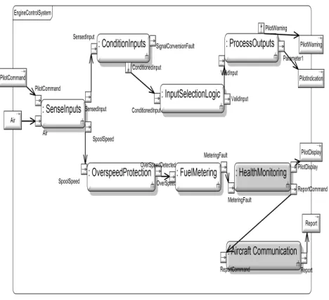
After creating the variability model, the next step is build-ing the base requirement model. For functional requirement modelling, SysML Activity Diagrams are used.

de-Figure 5. Functional requirement base model

Figure 6. Physical requirement base model

Figure 7. Non-Functional requirements representation

scribed in M. Dowding [44], and this paper treats this existing work as a legacy model. Because of the advantage of the or-thogonal variability modelling method, the original model does not require significant changes, just the addition of new variable elements. In this case, the variable requirements are “Health Monitoring” and “Aircraft Communication” and are highlighted in grey in Figure 5. After the creation of the func-tional requirement base model, the next step is linking the variants and variation points to the base model. For example, the variant “Health Monitoring” in the variability model links with the activity “Health Monitoring” via the artefact depend-ency concept in the meta-model.

Similarly, the physical requirements base model is mod-elled using a SysML Block Definition Diagram, as illustrated in Figure 6. The legacy models are kept the same. The variants are introduced by adding alternatives to the physical require-ment base model, then linking variable blocks to variation points and variants. The variable physical requirements are highlighted in grey in Figure 6.

Figure 7 shows how to represent the variability of non-functional requirements on each non-functional and physical re-quirement. As is shown, the stereotype <<Performance>> has “MinResponse” and “MaxResponse” implemented on func-tional requirements. “MinResponse” refers to the minimum response time and “MaxResponse” means the maximum re-sponse time. The variable performance attributes are repre-sented by modelling the performance attributes of variants. Reliability requirements are presented by applying the stereo-type <<Reliability>> to the blocks of the physical require-ments diagram. The tag “Failure Probability” shows the chance of failure occurring in a certain resource. After the implementation of these stereotypes, the next step is linking them to the associated variants. With regards to non-functional attribute analysis, this is still in a development stage. However,

traditional single system methods (without reusability), such as RBA [50] for timing analysis, can be used after each indi-vidual target system has been derived from the product line model this method creates.

D. Modelling Tool

Arti-san Studio also supports Embedded Real-Time System Model-ling with SysML, which is used as a base model in the pro-posed method. It is worth highlighting that the tool is ad-vanced in terms of product derivations. Unlike tools that re-quire the manual deletion of unselected options, users can select from the proposed variability models in Artisan and automatically derive the target system’s requirements.

V.DISCUSSION

This paper’s proposal mainly provides a practical method that can cope with the challenge of combining Software PLE with MBSE for Embedded RTS during the domain require-ment engineering stage. It is illustrated by a meta-model and implemented by extending OVM with stereotypes (Figures 3 and 4). Therefore it can be adopted by any tool that supports OVM. The result of this method is a domain requirement model (e.g. all models introduced in the case study section), which can be used to derive the target system’s requirements by configuring variants according to the specific requirements of customers. Methods for automatically generating a target system’s design and products will be the subject of future work by the authors.

Variability modelling assignment is based on the OVM method but extends it to support requirement engineering for Embedded RTS. According to V. Alves, N. Niu, C. Alves and G. Valença [10], the most commonly used variability model-ling methods are feature-based methods. Different approaches based on feature concepts have been proposed during the last two decades for solving different research challenges. Howev-er, all these approaches face limitations when they are imple-mented in large-scale companies, as feature-based methods have to represent both commonality and variability. In con-trast, OVM only represents variable parts, which reduces the number of elements that need to be described for variability modelling. Moreover, OVM supports the representation of variability in a separate diagram. It reduces the effort required to upgrade non-reusable legacies to PLE models.

Although OVM has a flexible design so it is able to com-bine with any type of modelling language diagram, it was pro-posed for the software domain. In the OVM proposal [22], different examples are illustrated that variants in variability models can be linked with different UML diagrams for re-quirement engineering. These variants are sometimes physical variants, such as “Colour Camera Surveillance”, “B/W Cam-era Surveillance” or “Infrared Surveillance”, and are linked with UML Use-case Diagrams, Sequence Diagrams, Class Diagrams and Data Flow Diagrams. It cannot be denied that physical resources have an impact on software design. How-ever, this is not enough for Systems Engineering, as physical resources should be detailed in interfaces and their connec-tions. It leads to physical variability in terms of physical inter-faces and connections. The original OVM links these physical options with software or functional options via artefact de-pendencies. This is confusing, because physical variants should be linked to physical artefacts. In addition, it leads to the problem of product line engineers having to analyse all physical, functional and non-functional interactions at the

be-ginning of PLE. For a large-scale company, which has thou-sands of variants, it is impossible to carry out this analysis at the beginning stage. Therefore this paper proposes a concept that represents different types of variability separately. The engineers who are responsible for physical variability only handle physical variable models and related low-level arte-facts. Engineers’ specifications are also extended by the pro-posed method to cope with the challenge of multiple stake-holders’ representations that is identified in [10].

Variability does not only exist between different systems. This paper’s proposed method copes with the evolution chal-lenge of variability modelling (identified in OVM [22] and [38]) by introducing a specification of variants’ usage periods. This paper is not the first to use MBSE with SPLE (such as related works [34] [35]). However, it is different from oth-ers that focus on how to combine existing variability model-ling methods with MBSE, as it focuses on modifying existing variability modelling methods to support MBSE in the re-quirement stage. Moreover, the Embedded RTS is different from other related works’ research contexts as the temporal requirements play an important role. This paper also provides a glimpse of how to handle non-functional variability, which is a challenge to OVM [22]. Detailed timing attribute analysis is the next stage of research. Unlike traditional MBSE, the paper proposes directly using SysML Activity Diagrams and Block Definition Diagrams in requirement engineering to re-duce the efforts involved in system design and increase the consistency of system models. The reason for this is that do-main requirement models can be directly used in the design stage by refining models for more detailed designs. The Rolls-Royce Control and Data Services team has defined an internal modelling standard for creating system and software require-ment models which uses the aforerequire-mentioned SysML activity modelling approach. The approach is now being applied in several civil aero-engine control system development projects. Early benefits are being seen in terms of reduced numbers of requirements expressing the same functionality as legacy text-based requirements capture. Reduced reworking at the system-software requirement handover stage is also apparent, arising from the alignment of the SysML activity model used for the capture of system requirements allocated to software with the underlying software architecture model (expressed in UML).

VI.CONCLUSIONS AND FUTURE WORKS

Product Line Engineering can be applied to Embedded RTS development to reduce the costs and schedules [33]. Re-quirement engineering is critical for Embedded Real-Time Systems, as a good requirement plan leads to less changes and risks being identified during the implementation stage. How-ever, current Product Line Engineering methods mainly focus on the software domain. The Embedded RTS domain is broader than the software domain in that physical require-ments and non-functional requirerequire-ments (Quality of Service attributes) play important roles.

The proposed method extends OVM, which has the advantage of reducing the efforts of introducing variability into existing documents. More specifically, it extends OVM with the sup-port of not only the separation of types of variation points and variants, but also representation of the evolution of variability. In addition, stakeholders’ information specifications are also covered by the proposed method in that it allows the identifi-cation of which role is responsible for certain down-selection decisions. Unlike traditional SysML modelling methods, this paper suggests directly using Activity Diagrams, stereotypes and Block Definition Diagrams to model functional, non-functional and physical requirements. In this way, it increases model consistency, as the requirements and system design are carried out using the same kind of diagram. The proposed method is illustrated by the Aircraft Engine Control System.

The challenge of combining Model-Based System Engi-neering with variability modelling in the design stage and ways of implementing quality analysis are the next stage of this work.

ACKNOWLEDGMENT

The author would like to thank Rolls-Royce Controls and Data Services team who are supporting the current research. Special thanks also go to Atego for providing a licence for the modelling tool Artisan Studio.

REFERENCES

[1] Friedenthal, S., Moore, A., & Steiner, R. (2008). A Practical Guide to SysML: Systems Modeling Language.

[2] Fortune, J. (2009). Estimating systems engineering reuse with the constructive systems engineering cost model. In Angeles, University of Southern California. Doctor of Philosophy. [3] Clements, P., & Northrop, L. (2002). Software product lines:

practices and patterns.

[4] van der Linden, F. J., Schmid, K., & Rommes, E. (2007). figureSoftware product lines in action: the best industrial practice in product line engineering. Springer Science & Business Media.

[5] Van Gurp, J., Bosch, J., & Svahnberg, M. (2001). On the notion of variability in software product lines. In Software Architecture, 2001. Proceedings. Working IEEE/IFIP Conference on (pp. 45-54). IEEE.

[6] Kang, K. C., Cohen, S. G., Hess, J. A., Novak, W. E., & Peterson, A. S. (1990). Feature-oriented domain analysis

(FODA) feasibility study (No. CMU/SEI-90-TR-21).

CARNEGIE-MELLON UNIV PITTSBURGH PA

SOFTWARE ENGINEERING INST.

[7] Chen, L., & Babar, M. A. (2011). A systematic review of evaluation of variability management approaches in software product lines. Information and Software Technology, 53(4), 344-362.

[8] Chen, L., Ali Babar, M., & Ali, N. (2009, August). Variability management in software product lines: a systematic review. In Proceedings of the 13th International Software Product Line Conference (pp. 81-90). Carnegie Mellon University.

[9] Metzger, A., & Pohl, K. (2014, May). Software product line engineering and variability management: Achievements and challenges. In Proceedings of the on Future of Software Engineering (pp. 70-84). ACM.

[10]Alves, V., Niu, N., Alves, C., & Valença, G. (2010). Requirements engineering for software product lines: A systematic literature review. Information and Software Technology, 52(8), 806-820.

[11]Czarnecki, K., Grünbacher, P., Rabiser, R., Schmid, K., & Wąsowski, A. (2012, January). Cool features and tough decisions: a comparison of variability modelling approaches. In Proceedings of the sixth international workshop on variability modelling of software-intensive systems (pp. 173-182). ACM. [12]Dumitrescu, C., Mazo, R., Salinesi, C., & Dauron, A. (2013,

August). Bridging the gap between product lines and systems engineering: an experience in variability management for automotive model based systems engineering. In Proceedings of the 17th International Software Product Line Conference (pp. 254-263). ACM.

[13]Kopetz, H. (2011). Real-time systems: design principles for distributed embedded applications. Springer Science & Business Media.

[14]Belategi, L., Sagardui, G., & Etxeberria, L. (2011, May). Model based analysis process for embedded software product lines. In Proceedings of the 2011 International Conference on Software and Systems Process (pp. 53-62). ACM.

[15]Myllärniemi, V., Savolainen, J., Raatikainen, M., & Männistö, T. (2015). Performance variability in software product lines: proposing theories from a case study. Empirical Software Engineering, 1-47.

[16]Myllärniemi, V., Raatikainen, M., & Männistö, T. (2012, September). A systematically conducted literature review: quality attribute variability in software product lines. In Proceedings of the 16th International Software Product Line Conference-Volume 1 (pp. 41-45). ACM.

[17]Metzger, A., Pohl, K., Heymans, P., Schobbens, P., & Saval, G. (2007, October). Disambiguating the documentation of variability in software product lines: A separation of concerns, formalization and automated analysis. In Requirements Engineering Conference, 2007. RE'07. 15th IEEE International (pp. 243-253). IEEE.

[18]Sepúlveda, S., Cares, C., & Cachero, C. (2012, June). Towards a unified feature meta-model: A systematic comparison of feature languages. In Information Systems and Technologies (CISTI), 2012 7th Iberian Conference on (pp. 1-7). IEEE. [19]Czarnecki, K., & Wasowski, A. (2007, September). Feature

diagrams and logics: There and back again. In Software Product Line Conference, 2007. SPLC 2007. 11th International (pp. 23-34). IEEE.

[20]Reinhartz-Berger, I., & Figl, K. (2014, September). Comprehensibility of orthogonal variability modelling languages: the cases of CVL and OVM. In Proceedings of the 18th International Software Product Line Conference-Volume 1 (pp. 42-51). ACM.

[21]Góngora, H. G. C., Ferrogalini, M., & Moreau, C. (2015). How to Boost Product Line Engineering with MBSE-A Case Study of a Rolling Stock Product Line. In Complex Systems Design & Management (pp. 239-256). Springer International Publishing.

[22]Böckle, G., & van der Linden, F. J. (2005). Software product line engineering: foundations, principles and techniques. K. Pohl (Ed.). Springer Science & Business Media.

Line Conference, 2008. SPLC'08. 12th International (pp. 139-148). IEEE.

[24]Rashid, M., Anwar, M. W., & Khan, A. M. (2015). Towards the Tools Selection in Model Based System Engineering for Embedded Systems-A Systematic Literature Review. Journal of Systems and Software.

[25]Jarraya, Y., Soeanu, A., Debbabi, M., & Hassaine, F. (2007, March). Automatic verification and performance analysis of time-constrained SysML Activity Diagrams. In Engineering of Computer-Based Systems, 2007. ECBS'07. 14th Annual IEEE International Conference and Workshops on the (pp. 515-522). IEEE.

[26]Andrade, E., Maciel, P., Callou, G., & Nogueira, B. (2009, February). A methodology for mapping SysML Activity Diagram to time petri net for requirement validation of embedded real-time systems with energy constraints. In Digital Society, 2009. ICDS'09. Third International Conference on (pp. 266-271). IEEE.

[27]OMG. (2008). UML profile for MARTE: Modelling and analysis of real-time embedded systems (Beta 2 ed.) Object Management Group Inc.

[28]Bagheri, E., Asadi, M., Gasevic, D., & Soltani, S. (2010). Stratified analytic hierarchy process: Prioritization and selection of software features. In Software Product Lines: Going Beyond (pp. 300-315). Springer Berlin Heidelberg. [29]Etxeberria, L., & Sagardui, G. (2008, September). Variability

driven quality evaluation in software product lines. In Software Product Line Conference, 2008. SPLC'08. 12th International (pp. 243-252). IEEE.

[30]Belategi, L., Sagardui, G., & Etxeberria, L. (2011, May). Model based analysis process for embedded software product lines. In Proceedings of the 2011 International Conference on Software and Systems Process (pp. 53-62). ACM.

[31]Ali, S., Yue, T., Briand, L., & Walawege, S. (2012). A product line modelling and configuration methodology to support model-based testing: an industrial case study (pp. 726-742). Springer Berlin Heidelberg.

[32]Trujillo, S., Garate, J. M., Lopez-Herrejon, R. E., Mendialdua, X., Rosado, A., Egyed, A., & De Sosa, J. (2010). Coping with variability in model-based systems engineering: An experience in green energy. In Modelling Foundations and Applications (pp. 293-304). Springer Berlin Heidelberg.

[33]Dumitrescu, C., Tessier, P., Salinesi, C., Gerard, S., Dauron, A., & Mazo, R. (2014). Capturing variability in model based systems engineering. In Complex Systems Design & Management (pp. 125-139). Springer International Publishing. [34]Huhn, M., & Bessling, S. (2013). Enhancing product line

development by safety requirements and verification. In Foundations of Health Information Engineering and Systems (pp. 37-54). Springer Berlin Heidelberg.

[35]Queiroz, P., & Braga, R. (2014). Combining MARTE-UML, SysML and CVL to build unmanned aerial vehicles. The Ninth International Conference on Software Engineering Advances, Nice, France. 334-340.

[36]Hallerbach, A., Bauer, T., & Reichert, M. (2010). Capturing variability in business process models: the Provop approach. Journal of Software Maintenance and Evolution: Research and Practice, 22(6-7), 519-546.

[37]Sellier, D., Mannion, M., & Mansell, J. X. (2008). Managing requirements inter-dependency for software product line derivation. Requirements engineering, 13(4), 299-313.

[38]Chen, L., & Babar, M. A. (2010). Variability management in software product lines: an investigation of contemporary industrial challenges. In Software Product Lines: Going Beyond (pp. 166-180). Springer Berlin Heidelberg.

[39]Seidewitz, E. (2003). What models mean. IEEE software, 20(5), 26-32.

[40]Bosch, J. (2005). Software product families in Nokia. In Software Product Lines (pp. 2-6). Springer Berlin Heidelberg. [41]Habli, I., Kelly, T., & Hopkins, I. (2007, September).

Challenges of establishing a software product line for an aerospace engine monitoring system. In Software Product Line Conference, 2007. SPLC 2007. 11th International (pp. 193-202). IEEE.

[42]Jaw, L. C., & Mattingly, J. D. (2009). Aircraft engine controls: design, system analysis, and health monitoring. American Institute of Aeronautics and Astronautics.

[43]Habli, I. (2009). Model-based assurance of safety-critical product lines (Doctoral dissertation, University of York). [44]Dowding, M. (2002). Maintenance of the Certification Basis

for a Distributed Control System–Developing a Safety Case Architecture. MSc Report, Department of Computer Science, University of York, UK.

[45]Atego. (2015). Artisan studio. Retrieved from

http://www.atego.com/download-center/products/category/ artisan-studio/

[46]ISO. (2013). ISO/IEC 26550:2013 Software and systems Engineering—Reference model for product line engineering and management ISO International Standards.

[47]Bashroush, R., Spence, I., Kilpatrick, P., Brown, J., & Gillan, C. (2008). A multiple views model for variability management in software product lines.

[48]Ali, R., Dalpiaz, F., & Giorgini, P. (2010). A goal-based framework for contextual requirements modelling and analysis. Requirements Engineering, 15(4), 439-458.

[49]Sinnema, M., Deelstra, S., Nijhuis, J., & Bosch, J. (2004). Covamof: A framework for modelling variability in software product families. In Software Product Lines (pp. 197-213). Springer Berlin Heidelberg.

[50]Grigg, A., & Guan, L. A Scalable Approach to Real-Time System Timing Analysis.

[51]Aainsqatsi, K. (2008). File:Turbofan operation lbp.svg.

Retrieved 7/30, 2015, from