Article
Applying Multi-Output Random Forest Models to
Electricity Price Forecast
Camino González *, José M. Mira and José A. Ojeda
Statistical Laboratory, Technical University of Madrid, 28006 Madrid, Spain; [email protected] (J.M.M.); [email protected] (J.A.O.)
* Correspondence: [email protected]; Tel.: +34-91-336-3149
Abstract: Predicting electricity prices is a very important issue in modern society, because the associated decision process under uncertainty requires accurate forecasts for the economic agents involved. In this paper, we apply the decision tree extension of Random Forests to the prediction of electricity prices in Spain, but with the novelty of modeling prices jointly with demand, with the purpose of achieving greater accuracy than with univariate response Random Forests, particularly in price prediction, as well as understanding the effect of the input variables (lagged values of price and demand, current production levels of available energy sources) on the joint of the two outputs. The results are very encouraging, providing significant increase in price prediction accuracy. Also, interesting methodological challenges appear as far as the appropriate choice of the relative weights of price and demand in the joint modeling is concerned and a new procedure to provide the importance variable ranking is proposed. The partykit (package of R software) library allowing for multivariate Random Forests has been used.
Keywords: electricity markets; price forecasting; multi-output models; random forests; conditional inference trees
1. Introduction
In any developed society, energy is a primary resource. Energy supply can be considered essential, ensuring wellness, stability and development.
Nowadays, in a global and interconnected society, energy supply can be considered a market where countries and public and private companies are capable of selling and buying energy according to their needs. The energy market involves three key elements: generation of electricity, transport, transmission, distribution and selling it to the consumer.
For energy generation, forecasting has become indispensable. The emergence of renewable energies (especially due to the policy applied in Spain since 2007) and their trend to become the main source of energy is an additional source of difficulty for the traditional energy producers to adjust their production. Traditional energy production includes thermal power plants and combined cycle, which are much more pollutant than renewable energies such as wind farms or solar energy. In the Spanish electrical market renewable energies are part of Special Regime [1] and generally, facilities that produce renewable energy have a maximum installed capacity of 50MW.
Pollutant ways of energy production are currently used for demand not covered by renewable sources. Due to the variability of renewable resources (such as wind), a reliable energy production system should lean on thermal power plants and combined cycle, which can adjust their productions almost instantly when necessary.
The Spanish energy market is specially complex since it adjusts energy prices using a “pool market”: prices are fixed at the figure at which the last producer used to cover demand offers energy. This means that, although some producers can offer their energy at price 0 €/MWh, they still get paid for this energy as long as price for the last energy used is not zero €/MWh, [2]. For this reason, renewable energy producers offer their energy at 0€/MWh, and the rest of producers fix their prices according to demand. This explains that renewable energies are always chosen to cover demand. Therefore, price forecasting is also a main issue for energy producers and by thus for the energy market.
Although current models for price and demand forecasting are well developed and mature, there is still room for new research. New approaches provide new accurate models for price and demand forecasting, a better understanding of the energy market and steady improvement of already existent models.
Some of the current models for price and demand forecast are based on the ARMA-ARIMA methodology [3-12]. Others incorporate exponential smoothing [12-14] and data mining techniques [15-22]. These analyses are performed for short, medium and even long term and separately for each variable: price and demand, since the importance variables are different.
Only the work of Amjadi and Dareeepour [23] deals with the joint study of price and demand using an iterative neural network procedure and provides results for different electricity markets including the Spanish one.
When building a forecasting model, it is important to take account of the following:
• The input variables used for the analysis should be appropriate for the specific response. Variable importance measures are often used to determine which variables should be included in the models.
• Forecasting is often performed for very short horizons, e.g. one hour ahead, a day ahead, so predictions should be obtained quickly.
The approach in this study consists in the use of decision tree algorithms (Random Forests) [24] and of multivariate analysis, i.e. joint analysis and one hour ahead forecast of price and demand. One of the key points in the method is the selection of the explanatory variables. It is clear that in the new Spanish context, where since 2007 the renewables energies have been extensively introduced in the market, the identification and evaluation of importance variables through a variable ranking is crucial and Random Forests (RF from now on) provide it. Besides, it is clear that prices are load dependent, but in the new regulatory scenario, load patterns (customers behavior) should be also affected by electricity prices. This is the main reason for the use of the multioutput approach based on RF.
This allows us to test other models for the energy market and to take advantage of the correlation between responses (price and demand) and to find relationships between the responses and the input variables of the market, which may prove useful to develop or improve other models. In addition, the predictive performance of multivariate RF is tested as an alternative to univariate RF models. [19]
For this paper, 2013 and 2014 hourly energy Spanish market data has been used [2]. There are three kinds of energy market variables: calendar variables (related to the date, hour and type of day), present and lagged values of price and demand, and energy production variables, i.e. MWh of each kind of energy consumed along each hour.
2. Theoretical Framework
The scope of this article relies on regression tree based models in particular RF models and especially in the more recent development of multi output RF models. In what follows a brief description of the main features is provided.
2.1. Random Forests
RF is a tree-based method for classification and regression consisting in an ensemble of individual decision trees. The trees used as base learners in RF can be of different types (i.e. CART [25], C4.5 [26], or Conditional Inference [27]). In this paper, the individual trees used have been Conditional Inference Trees (CI Trees), since the algorithm provided by Hothorn (Party and Partykit libraries in R [28]), allows for multivariate, multi-output analysis.
As Hothorn and Zeileis [27] write, CART and C4.5 have two fundamental problems: overfitting and a selection bias towards covariates with many possible splits, which will lead to a biased importance ranking. In non-CI trees, to avoid overfitting, the trees created are pruned, however, the bias (induced by maximizing a splitting criterion over all possible splits simultaneously) is not so easy to eliminate.
CI Trees are capable of overriding this problem using a statistical approach which takes into account the distributional properties, measuring in a first step the association between responses and covariates. This means that the iterative binary partitioning and the stopping criteria are applied with multiple test procedures to determine whether or not a significant association exists between any of the covariates and the response. Here, in similar fashion to contingency table independence tests, the association between the sign of model residuals and each covariate is measured by a P-value derived from a permutation test (null hypothesis test of independence between each covariate and the response variable, following standard test of independence). This implementation decreases bias and overfitting problems, and trees are created of different sizes (depth) depending on the pre-specified significance level α. A brief description of CI Tree modelling, based on [27] is presented as follows:
Input variables and response are defined as well and may have arbitrary scales:
• Response variable Y (possibly multivariate, in our paper bivariate response variable).
• Covariate vector X=(X1,…,Xm) taken from a sample space X = X 1×…× X m. Obviously covariates
are the input variables for the model.
The conditional distribution of the response Y given covariates X depends on a function fof the covariates:
D(Y|X)=D(Y|X1,…,Xm)=D(Y|f(X1,…,Xm).
Binary partitioning is implemented using a case weight vector w=(w1,…,wn), where n is the
sample size. Each node of the tree is represented by its own vector of case weights, w (non-zero elements when the corresponding observations i (Yi) are elements of the node and zero otherwise).
For w, the global null hypothesis of independence between any of covariates Xj and the
response Y is tested. If the hypothesis cannot be rejected, the splitting stops. Otherwise, the covariate
Xj*with the strongest association to Y is selected.
Set A ∈ Xj* is chosen in order to split Xj* into two subsets, left = {A* / Xj*<A*} and right = {Xj* > A*}. This creates two new case weight vectors: wleft and wright. These steps are performed iteratively
until the algorithm cannot reject the null hypothesis and the algorithm stops.
The association between Y and the covariate Xj is measured, for the test, by a linear statistic Tj ,
whose expression is [27]:
( , ) = (∑ ℎ , ( , … , ) ʈ∈ R , (1)
where:
• is a learning sample, possibly with some covariates missing.
• gj :Xj→ Rpj is a non-random transformation of the covariate Xj .
The step forward from individual CI Trees to an ensemble is the RF-CI algorithm. In RF, each tree (base learner) in a forest is developed by employing two sources of randomness, thus decreasing correlation between trees and building a more reliable algorithm [29].The two sources stem from:
• The samples used to build each tree are randomly selected from a given training dataset.
• The variables used to build each tree are also randomly selected from the total set of input variables available. The algorithm is not allowed to consider every predictor (variable) available, in such way that the not-very-strong predictors may appear in the top splits and preventing the trees from being very similar and thus from producing highly correlated predictions.
Thus, the trees can be regarded as near independent. When many nearly independent trees are combined for analysis, the risks of biased decisions or overfitting would decrease greatly, also variance of prediction decreases. As a consequence, RF, in particular CI based, has been recognized as an effective method in machine learning and as an algorithm which provides accurate predictions for many classification and regression problems.
2.2. Specific Issues for Multi-Output Analysis
There are two general approaches for solving multi-output pattern recognition problems: either by transforming the problem into multiple single-output problems; or by adapting a pattern recognition algorithm so that it directly handles multi-output data [30]. When the datasets are large enough, performing a regression or classification model becomes very expensive in terms of computational resources. Therefore, when many models need to be obtained from the same dataset, it could be useful to perform a single multivariate analysis with two or more responses (outputs) from the same dataset instead of performing two or more univariate analyses separately, since the computation times are thus nearly halved.
More importantly, when the predictions are cross-correlated, training a coherent multi-output model can potentially increase predictive performance compared to training multiple disjoint models [31].
In this paper the research focuses on a multi-output regression problem, since both price and demand are continuous variables. When predicting, the univariate (single output) and multivariate (multi-output) approaches will be compared in this research, focusing not only on the accuracy of predictions but also on computing times.
In general terms, multi-output models based on RF build trees using the variables that explain both response variables for recursive binary splits. This approach means that the influence of each variable should be tested with the hypothesis tests of independence (mechanism used in CI trees) for each response variable. For this reason, the mathematical complexity of multivariate analysis is higher than for the univariate case.
As the response Y is multivariate, each observation Yi will contain two or more responses.
Therefore, the global influence function h (as appears in Eq. (1)), depends on the multivariate response variables (demand and price in our research).
2.3. Importance Variable in Multi-output Environment. New Proposal
A summary of the importance of each input variable can be obtained using the Mean Squared Error (MSE) criterion. Grömping [32] uses the Out-of-Bag (OOB) concept and a permutation-based test to evaluate MSE reduction. As explained in [19], for each tree in the forest, built with a learning data set (usually about two-thirds of the observations), the value of a variable Xj which has been used to build the tree, is randomly permuted in the OOB data set (about one-third of the observations), and a new value of the MSE in the OOB is calculated. The importance of the variable is computed from the differences between MSE and MSEpermuted according to the expression:
̅ = 1 ( − ) =1 ,
= ∑ ( − ) .
Afterwards, ̅ is normalized with the standard error and the final value of the importance metrics is obtained as follows:
% = ̅
√ .
If the Xj variable does not have predictive importance on the response, is almost zero, therefore
the higher is the value of %IncMSEj, the higher is the importance of the variable.
However, due to the novelty of the algorithm and the early stage of development of the partykit
library [33], there are no specific commands to evaluate variable importance, for either the univariate response or the multivariate response. Additionally, it is difficult to access each tree in the RF, thus complicating the use of the approach proposed by Grömping [32], mentioned above.
For these reasons, a more pragmatic approach has been developed and proposed here, consisting in permuting an explanatory variable at a time with both responses simultaneously and evaluating the evolution of MSE of the whole RF. In fact this could be considered as a generalization of the previous algorithm. It is important to note that the results provided by this method are not the same as those of from using the permutation for each tree individually instead for the whole forest.
On the other hand, taking into account that multivariate analysis is performed, using MSE to evaluate error is useful when analyzing response variables separately, but it is not appropriate to compute a joint error unless a function of both response variables is created. This is the reason for the following proposal of the study: the definition of a joint response function involving both price and demand.
Since price is usually higher (three orders of magnitude) and harder to predict than demand, it is expected that price error has more influence than demand error when using a price-demand dependent function. This should condition the relative weights of both outputs. For these reasons, the price-demand dependent function proposed to be used as response variable in the analysis of this paper is:
− ( , ) = ( )( € ). (2)
This function makes similar order magnitude for price and demand and marks price as the most important response variable (in the denominator, log 10 smooths error for demand).
Evaluating a joint MSE using this function has some implications:
• The MSE can be smaller when an input variable (explanatory variable) is removed. This means that removing a specific input variable improves price prediction allowing price-related input variables to appear more often. This improvement can occur for price and demand simultaneously or in exchange for less accurate demand prediction. This happens especially when no highly important demand-related input variables are removed (removing very important demand predictors will result in an increase of the joint MSE).
• Some variables can be important for price or demand when evaluated separately, but removing these variables does not imply a loss of accuracy if removed one by one. The reason is that other not-so-important variables are capable of holding the quality of predictions if only one important variable is permuted.
• Removing some of the inputs which are less relevant in the joint (multivariate) analysis, will certainly result in an improvement of price prediction and could also improve demand predictions. However, in some cases this removal could result in a loss of accuracy in demand predictions larger than the corresponding improvement in price predictions averaged over the full sample. This behavior is not frequent but should be born in mind
2.4. Ajusting Tuning Parameters for The Study
The main tuning parameters in a RF algorithm are the number of trees of the forest (ntree), the number of variables (mtry) randomly chosen to be considered for each split in the individual trees and the depth of every individual tree. The adequate selection of these parameters could significantly improve the performance accuracy of the models, but the choice of the optimal values is case study-dependent.
In this section the importance and influence of these tuning parameters have been studied considering that input and response variables correspond to the same time point.
The algorithm used in our approach is included in the R “partykit” library [33]. The RF-CI algorithm allows the user to choose the type of test statistic to be applied and how to compute the distribution of the test statistic. For this data set and multivariate framework, a computational study has determined that the best results are obtained using teststat=”quad” and testtype=“Teststatistic”.
All plots and charts have been created using the R “ggplot2” [34] library, since “partykit” does not include plot functions yet due to its early stage of development.
2.4.1. Depth of Individual Trees
The depth of each individual tree can be either adjusted manually or have the algorithm choose it automatically. When trees grow too deep, there appears the risk of overfitting. As said before, the parameter α, specified in the construction of the algorithm, refers to the level of significance for the input-output independence tests, and is directly related to the depth of the trees. The higher the value of α, the less difficult to reject independence and thus a split which would result in a greater depth [27]. In this paper, the α-value has been chosen at 0,05, a standard value for this parameter that ensures trees do not grow too deep.
2.4.2. Number of Trees in The Forest (ntree)
The number of trees used to make the ensemble, has a direct influence in prediction accuracy. The higher the number of trees, the smaller the error. But this trend is asymptotic: if the number of trees is large enough, increasing the number of trees does not result in a significant improvement in predictions. Besides, using more trees requires larger computing times. For this reason, the number of trees is set based on a trade-off solution between computing time and predictive performance.
For the study of the influence in the error of the number of trees in a RF-CI, how the error is computed should be defined first. In this section, the standard metric Mean Squared Error (MSE) of the Oot-Of-Bag (OOB) predictions for each response (output variable) has been first used to evaluate prediction accuracy.
Each tree makes use of around two-thirds (63,2%) of the observations to build the tree. The remaining observations are referred to as OOB. One may predict the response for the ith observation using each of the trees in which these observation is OOB. The accuracy of a RF prediction can be estimated from these OOB data as in [32]:
− = ∑ ( − ) ,
where n is the sample size, the actual value of the observation and is the average prediction for the ith observation from all trees for which this observation has been OOB.
Figure 1. OOB-MSE for Demand versus the number of trees in the forest.
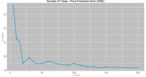
Figure 2. OOB-MSE for Price versus the number of trees in the forest.
As it can be observed, for both responses, the decrease of the error starts to stabilize at 100 trees approximately; for example, the error difference is small when comparing 150 and 200 trees. Seeking for a trade-off solution, the number of trees when making predictions has finally been set at 150.
2.4.3. Number of variables randomly selected to be considered at each split (mtry) in RF
To choose the value of the mtry parameter it is necessary to consider the correlation between the input variables. With highly correlated input variables it is preferable to use a small value [29]. Traditionally, mtry=√p for classification forests and mtry=p/3 for regression forests (where p is the total number of input variables) [32].
On the other hand, if there are many irrelevant input variables, a larger value of mtry would be needed in order to obtain better predictions. In this study, initially, there seem to exist input variables that may be irrelevant (or at least of relatively minor importance). An input variable highly uncorrelated with the remaining inputs, could be very important due its unique behavior in the analysis or not important at all in the prediction if not related with the response.
Figure 3 shows the Pearson correlation between the input variables.
Since, as may be observed from the Figure 3, the correlations between the input variables are in general low and it is plausible (a priori) that some input variables are of low relevance, the mtry
parameter could be chosen higher than recommended [32]. RF-CI will likely have stopped splitting before the weak predictors (input variables) come into play with larger mtry [32].
An analysis has been performed to determine the optimal value for the mtry parameter. Since the number of input variables is p=14, the study range for the mtry parameter has been from 5 to 10. This analysis has been performed with a RF-CI of 50 trees, OOB predictions, 3000 observations and it has been replicated 10 times.
The evolution of the OOB-MSE for demand and price as mtry grows is displayed in Figures 4 and 5.
Figure 4. Selection of mtry parameter: Evolution of OOB-MSE (mean of 10 replications) for demand.
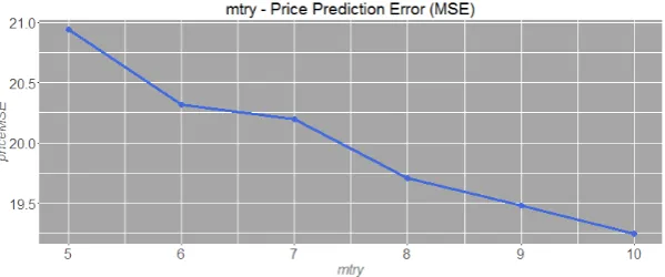
Figure 5. Selection of mtry parameter: Evolution of OOB-MSE (mean of 10 replications) for price.
When mtry equals 7, the smallest error in demand prediction and a substantial reduction in price error prediction are obtained. Thus, the value of the mtry parameter has been set at 7, once again seeking for the best trade-off option: the minimum for demand and not so small for price.
Besides, the contemporaneous correlation between price and demand is 0.4512. This value is not high enough to establish a priori that multivariate analysis will result in more accurate predictions than individual univariate ones (as mentioned above, highly correlated responses imply better predictions when using multivariate analysis).
3. Application to the Spanish Electricity Market
cycle, hydraulic, wind and total special regime); besides calendar variables (type of day, day of the week, hour of the day and month) which incorporates in their different categories, information on the different price and demand patterns have been considered. The generation structure have been included in the data base to evaluate if the proposed methodology is able to capture market behavior, for example, some technologies are incorporated to the generation when high demand occurs and lead to high prices. Values of these variables are obtained from REE [1] and OMIE [2]. Table 1 summarizes their values.
Table 1. Variables included in the data base.
Variable Name Value
Type of day day.type 1=working day, 2=weekend
3=public holiday
Day of the week day.week 1-7 (days)
Hour of day hour 1-24 (hours)
Month month 1-12 (months)
Price price 0-115 €/MWh
Lagged Price one hour price.t1 0-115 €/MWh
Lagged Price two hours price.t2 0-115 €/MWh
Lagged Price twenty-four hours price.t24 0-115 €/MWh
Hydraulic Energy production hydr 420-12050 MWh
Nuclear Energy production nucl 3500-7125 MWh
Coal Energy production carb 390-9660 MWh
Fuel-gas Energy production fuel.gas 0-495 MWh
Combined cycle energy
production comb.cyc 330-12320 MWh
Wind Energy production eolic 1500-15000 MWh
Total renewable energy
production reg.special 3880-26415 MWh
Demand demand 17085-39965 MWh
3.1. Variable Importance Analysis
the more important is the variable. On the other side, the greater the decrease in the MSE, the less important the variable is so it could be removed from the analysis. B) A joint function of the responses (price and demand) is defined, and the MSE is computed for this bivariate response function.
In our study Eq. 2 has been defined as joint function but others functions could be tried in the future.
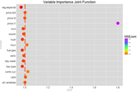
The computational study involves a RF-CI of 100 trees, 3000 observations each, mtry=7, α=0,05 and OOB predictions have been used to evaluate the variable importance. Values for th tuning parameters have been selected according to the study described in Section 2. The proposed methodology has been implemented both in the univariate and multivariate framework of the RF-CI to assess experimentally the consistency of such rankings. Figures 6 through 8 show the results in terms of the variation of the MSE for the whole RF for univariate price, univariate demand and joint function respectively (Eq. 2).
Figure 6. Variable importance analysis for price.
Figure 7. Variable importance analysis for demand.
In previous figures, the dashed vertical lines represent the MSE value of the RF-CI when all predictors maintain their true values. Predictors to the right of the dashed vertical line are significant and the higher is the value of MSE, the higher the importance of the variable, which means that if this variable is randomly permuted when building the forest, the MSE will increase. Unlike previous ones, predictors to the left of the dashed vertical line have a negative effect on the MSE, that is, if these variables are randomly permuted from the analysis, the MSE will decrease and a better prediction accuracy will be obtained. Furthermore, this result allows us to conclude that if these variables are eliminated from the analysis, the prediction improves. The values in Table 2 complete the information displayed in Figures 6 through 8.
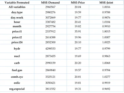
Table 2. Comparison of Mean Squared Errors.
Variable Permuted MSE-Demand MSE-Price MSE-Joint
All variables 2960567 20.04 1.0016
day.type 2980276 19.59 0.9788
day.week 3072869 19.77 0.9876
hour 3387482 20.41 1.0184
month 2927754 19.82 0.9910
price.t1 2337912 35.91 1.8015
price.t2 2614388 19.96 1.0007
price.t24 2852300 20.10 1.0025
hydr 4298533 19.77 0.9799
nucl 2873455 19.69 0.9863
carb 2990159 20.20 1.0068
fuel.gas 2869840 19.57 0.9784
comb.cyc 3325121 20.81 1.0277
eolic 3050421 19.81 0.9919
reg.especial 3811552 19.31 0.9692
For example, when explanatory variable price.t1 is randomly permuted, the OOB-MSE-Price increases to reach the highest value 35.91. Thus, the one hour lagged price (price.t1) is the most important variable to accurately predict the price. For demand, the most important variables are those related to the energy produced by the different technologies and used to cover demand instantly, i.e. renewable energies, combined cycle, and hydraulic as well as some calendar variables as the hour and the day type. Therefore, if the responses are considered separately, the univariate output approach,those input variables extremely related to one response are less important for the other (lagged prices are the less important for demand in RF-CI for example and hydraulic production for price in RF-CI).
Figures 6 through 8, and Table 2, with the exact values, indicate that multivariate importance variable analysis selects as the most important input variables those that explain each response separately (lagged values of price for price or hour for demand) and those that provide a good explanation of both response variables, energy produced by combined cycles (comb.cyc) for example. Summarizing,, the most important variables for both price and demand are one hour, two hours and 24 hour lagged prices, and energy produced by combined cycles and coal (comb.cyc and carb
except for renewable energy production (reg.especial), day type(day.type) and energy produced by fuel gas plants (fuel.gas). These variables have a slightly negative influence on the joint prediction when price is selected as the most important response variable in multioutput analysis.
It should be highlighted that, due to the definition of the joint importance function, joint variable importance is very similar to that of univariate price. If another joint function had been defined, for example, giving equal importance to price and demand, the results would have been different.
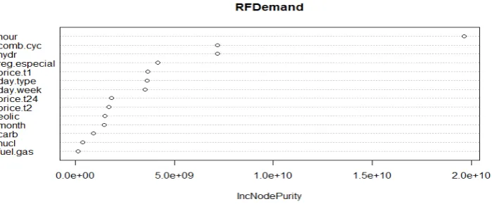
The previous results, as obtained from RF-CI, can be compared with those provided by non conditional RF-CART evaluated for each response separately and presented in Figures 9 and 10 for price and demand respectively. In these cases the function “varImpPlot” to evaluate variable importance included in the library RandomForest has been used and the importance measure based on the Gini index, IncNodePurity, is displayed. This measure quantifies for each explanatory variable, the average decrease in the forest of the Gini index.
Figure 9. Importance variable analysis for price using RFCART.
Figure 10. Importance variable analysis for demand using RFCART.
The results of variable importance for RF-CART are pretty similar, validating the approach proposed and followed for RF-CI.
3.2. Forecasting One Hour Ahead
The input variables are the set of exogenous variables previously defined in Section 3 and lagged responses including two new ones: one hour lagged predicted price and predicted demand. It is worthwhile to mention that input variables are the same for the two forecast processes: price and demand, as it is incorporated in the multi-output algorithm of partykit.
The strategy to perform predictions is to eliminate from the analysis those predictors identified as having a negative influence on the joint MSE (i.e if they are eliminated, accuracy will increase).
Thus, the input variables are a set of exogenous variables and lagged responses including two new ones: one hour lagged predicted price and predicted demand.
For a more representative analysis, for comparison purposes with similar analysis with alternatives models, the error metric has been changed. Adopting the MAPE error measurement provides better interpretability, clarifying forecast accuracy.
The MAPE (Mean Absolute Percentage Error) is defined as follows:
=1 | − |
Since price (and by extension, the denominator of price-demand function as defined previously) is zero for many observations, a MAPE cannot be used directly. Therefore, the so called Fixed MAPE has been used in price and for the price-demand function, using the mean of the present values in the denominator:
=1 | − |
Once again, the joint function defined in Eq. (2) has been used, as well as individual price and demand forecasts.
Due to its random-based construction, the RF-CI created with the same training data set may produce slightly different outputs. Moreover, using different training data sets produces more variability in the results, which, however, hardly change from one set of bootstrap samples to another, i.e, we achieve the robustness sought with the RF stabilizing effect. Both the best and worst forecasting results are presented, as follows, to compare with other results in particular those provided for the Spanish market.
For all analyses, RF of 150 trees, mtry=7 and α=0.05 have been used (as selected in previous sections). The total number of observations (hourly data corresponding to the Spanish electricity market for 2013 and 2014, 17520 registers) has been split into two data sets: training data set (12270 observations) and test data set (5250 observations). The length of the training data set has not be optimized, in future works, the influence of the length on the prediction accuracy will be analyzed.
The prediction performance of the models is summarized in Table 3.
Table 3. Comparison of MAPE errors for multivariate and univariate modelling.
Demand MAPE (%) Price MAPE* (%) Joint MAPE* (%)
MultivariateRF-CI
(Best joint RF) 3.0650 6.8967 6.7881 Multivariate RF-CI
(Worst joint RF) 3.0477 7.2241 7.1111
MultivariateRF-CI
NA 2.8299 6.8873 6.7881
Univariate RF-CI
(Best RF) 2.7943 7.4324
Univariate RF-CI
(Worst RF) 2.8676 7.4477
Univariate RF-CART
Univariate RF-CART
(Worst RF) 2.9598 8.0345
*Fixed MAPE
Removing variables that have a negative effect on the joint function error (as identified in the variable importance analysis explained in subsection 4.1) results in a reduction in both price and demand forecasting errors (Row “Multivariate RF-CI NA” in bold Table 3). This means that when carrying out the adequately the multivariate analysis, selecting input variables can favor forecasting for both responses. In our case, the variables related to renewable energy production, day type and fuel gas energy production have been removed, allowing other variables whose influence on the joint function is minor, to appear more often and thus improving the algorithm’s forecasting accuracy.
Note also that removing other variables whose influence is minor can result in a better price forecasting and a worse demand forecasting.
Finally, RF-CI and RF-CART have been used to perform univariate analysis for comparison with multivariate analysis using RF-CI, referred to as Univariate in Table 3. The comparison highlights that results are pretty similar for both techniques (RF-CI and RF-CART) and slightly different from those of the multivariate analysis.
Systematically, univariate RF-CART provides slightly higher errors than those of univariate RF CI. The best forecasting results come from Multivariate RF-CI when a previous input variable selection by variable importance analysis is carried out, and are quite similar to those of univariate RF-CI for demand, in fact the value obtained for the MAPE in the multivariate analysis for demand (2.8299) lies between the best (2.7943) and the worst results (2.8676).
In general terms, the results presented in Table 3 are similar. However, performing two univariate analyses requires doubling computing times, which for a single multivariate analysis is the same than those required to conduct one univariate analysis. Since forecasts presents almost the same accuracy, multivariate analysis can thus be considered more appropriate.
It is also noted that results of the multivariate forecast are more accurate for demand than for price, so the methodology is able to capture and reproduce results widely known in the literature.
When comparing the results of this research to those of studies relating to the Spanish electricity market performed with tree based models [19], and simultaneous prediction of load and price [23], the conclusion is that there are very promising.
Just for price, analysis carried out in [19] for the Spanish electricity market in 2011, shown a mean of MAPE for the third week of august of 6.02% (168 hours) obtained with RF-CART models. Amjady and Dareepour [23], for four specific weeks of 2002 for the Spanish system, report a MAPE of 4.22%, 4.39%, 5.55% and 5.66% respectively, with an algorithm that clearly outperforms other methods, with a MAPE mean ranged in the interval 6.76% to 9.96%. This comparison is presented in [23] and it includes time series and machine learning-based models.
Regarding load prediction, [23] reports for the same weeks in the Spanish market, 2002, a MAPE value of 0.99%, 1.10%, 1.02% and 1.08% respectively; and for January 2004 and July 2004 in the New York electricity market, they present 1.57% and 2.11% respectively which indicate better accuracy than other methods, as summarized in their paper as well, where MAPE varies from 1.82% to 3.55%.
So, as commented previously, results are good in terms of accuracy, in the same order of magnitude that other data mining models, although it is clear that new improvements in the methodology should be incorporated and the selection of tuning parameters to ensure the algorithm is reliable has been stated as essential.
4. Conclusions
RF-CI and decision tree algorithms come into play as a powerful, reliable and useful tool for data exploration, understanding and prediction. Results show that the methodology proposed and incorporated in the algorithm is able to find the main drivers for price and demand meaningfully. After the importance variable assessment the following conclusions can be outlined:
Due to the number of input variables and in some cases to their correlations, it is possible to remove some input variables without affecting prediction accuracy.
• Price. The most important variables for price are one hour lagged price, combined cycle energy production and hour. In most cases, removing only one variable does not imply a significant change and sometimes means a small improvement.
• Demand. The most important variables for demand are renewable energy production, hour, day type and combined cycle energy production. For demand, lagged prices are not important. Demand seems to present more instability than price when just one variable is removed, but the algorithm is still capable of providing good predictions using the rest of input variables.
• Joint-Prediction: due to the definition of the joint-prediction function, its behavior is very similar to that of price. In this case, removing some not-very influential variables allows other ones (hidden by previous ones) to appear often and improves predictions without modifying their quality. For joint prediction, the most important variables are those which appear as important variables for both price and demand. In the case of price.t1, it is not important for demand but extremely important for price, and it appears as the most important input variable for joint prediction.
Although the production of renewable energy results an important input variable for demand, its importance is minor for joint prediction. In fact, removing it results in an improvement. This can be explained by the high correlation between wind energy production and renewable energies that allows the algorithm to use wind energy as covariate instead of renewable energies without losing accuracy. This behavior highlights the importance of the study of correlation between input variables.
The analysis of variable importance and correlations is recommended since it allows for the identification of input variables that reduce the accuracy of predictions. In the future different joint functions should be tried.
Regarding forecast accuracy, the main conclusions can be summarized as follows:
The best results have been obtained using multivariate RF-CI combined with previous selection of input variables (i.e., removing those variables that decrease forecast accuracy). In this case, RF-CI emerges as a competitor for traditional forecasting algorithms, such as ARIMA techniques and provides results with similar accuracy results as other machine learning methods.
Using all variables in multivariate RF-CI provides similar results, with a slight loss of accuracy, especially for demand. Univariate analysis performs similarly for demand and worse for price, but the difference is positive and greater in the case of price.
Taking into account that the computational effort needed for conducting two univariate analyses is twice that of a single multivariate one, then, the later is preferable. Besides, selection of tuning parameters to ensure the algorithm is reliable has been stated as essential.
The results globally imply room for new methodological research and for new computational experiments to adjust some important issues of the algorithm such as the length of the training set and the meaningful selection of joint function.
Acknowledgments: This study was supported by the Spanish Ministry of Science and Innovation in the framework of the project Modelling and forecasting electricity and CO2 markets through unobserved components models (DPI2011-23500).
Conflicts of Interest: The authors declare no conflict of interest References
[1] REE:’ Spanish transmission system operator’, Available online: http://www.ree.es, (accessed 2016).
[2] OMIE:’ Spanish electricity price market operator’, Available online: http://www.omie.es , (accessed 2016).
[3] García-Martos, C.; Rodríguez, J.; Sánchez, M.J. Mixed models for short-run forecasting of electricity prices: Application for the Spanish market. IEEE Trans. Power Syst.2007, 22, 544-552. [4] García-Martos, C.; Rodríguez, J.; Sánchez, M.J. Forecasting electricity prices and their volatilities using unobserved components. Energy Economics 2011, 33, 1227-1239.
[5] Nogales, F.J.; Contreras, J.; Conejo, A.J., Espinola, R. Forecasting next-day electricity prices by time series models. IEEE Trans. Power Syst. 2002, 17, 342-348.
[6] Conejo, A.J.; Plazas, M.A.; Espinola, R.; Molina, A.B. Day-ahead electricity price forecasting using wavelet transform and ARIMA models. IEEE Trans. Power Syst.2005, 20, 1035-1042.
[7] Contreras, J.; Espinola, R.; Nogales, F.J.; Conejo, A.J. ARIMA models to predict next-day electricity prices. IEEE Trans. Power Syst.2003, 18, 1014-1020.
[8] Alonso, A.; García-Martos, C.; Rodríguez, J.; Sánchez, M.J. Seasonal dynamic factor analysis and bootstrap inference: Application to electricity market forecasting. Technometrics 2011, 53, 137-151. [9] García-Martos, C.; Rodríguez, J.; Sánchez, M.J. Forecasting electricity prices by extracting
dynamic common factors: application to the Iberian Market. IET Gener. Transm. Distrib. 2011, 1,1-10. [10] Alonso, A.M.; Bastos, G.; García-Martos, C. Electricity Price Forescasting by Averaging Dynamic Factor Models. Energies 2016, 9, 600, DOI: 10.3390/en9080600.
[11] Huang, S.J.; Shih, K.R. Short-term load forecasting via ARMA model identification including non-Gaussian process considerations. IEEE Trans. Power Syst.2003,18,2, 673-679.
[12] Taylor, J.W.; McSharry, P.E.. Short Term load forecasting Methods: An Evaluation based on European Data. IEEE Trans. Power Syst.2007, 22, 4, 2213-2219.
[13] Carpio, J; Juan, J.; López, D. Multivariate exponential smoothing and dynamic factor model applied to hourly electricity price analysis. Technometrics, DOI: 10.1080/ 00401706.2013. 860920. [14] Song, K.B.; Ha, S.K.; Park, J.W.; Kweon, D.J. ; Kim, K.H. Hybrid load forecasting method with analysis of temperature sensitivities. IEEE. Trans. Power Syst.2006, 21, 2, 869-876.
[15] Cataläo, J.P.S.; Pousinho, H.M.I.; Mendes, V.M.F. Short-term electricity prices forecasting in a competitive market by a hybrid intelligent approach. Energy Convers. Manag.2011, 52, 1061-1065. [16] Fan, S., Mao, C., Chen, L. Next-day electricity-price forecasting using a hybrid network, IET Gener. Transm. Distrib. 2007, 1, 1, 176-182.
[17] Amjady, N. and Daraeepour, A. Keynia, F. Day-ahead electricity price forecasting by modified relief algorithm and hybrid neural network. IET Gener. Transm. Distrib. 2010,4, 3, 432-444.
[18] Neupane, B.; Perera, K.S.; Aung, Z.; Woon, W.L. Artificial Neural Network-based electricity price forecasting for smart grid deployment. International conference on Computer Systems and Industrial Informatics (ICCSII) 18-20 December. 2012. ISBN: 978-1-4673-5155-3. DOI: 10.119/ICCSII.2012.6454392.
[19] González, C.; Mira-McWilliams, J.M.; Juárez, I. Importance variable assessment and electricity price forecasting based on regression tree models: classification and regression trees, Bagging and Random Forests,. IET Gener. Transm. Distrib. 2015, 9, 1120-1128.
[20] Fan, G.; Qing, S.; Wang, H.; Hong,W.; Li, H. Support Vector Regression Model Based on Empirical Mode Decomposition and Auto Regression for Electric Load Forecasting. Energies2013, 6, 1887-1901.
[21] Bozic, M.; Stojanovic, M.; Stajic, Z.; Tasic, D. A New Two –Stage Approach to Short Term Electrical Load Forecasting. Energies, 2013, 6, 2130-2148.
[23] Amjady, N. and Daraeepour, A. Mixed price and load forecasting of electricity markets by a new iterative prediction method. Electr.Power Syst. Res. 2009, 79, 1329-1336.
[24] Breiman, L. Random forests. Machine Learning2001, 45 , 5-32
[25] Breimann, L., Friedman, J.H., Olshem, J.H., Stone, C.J.: Classification and regression trees. Chapman and Hall/CRC, 1984.
[26] Quinlan, J. ‘C4. Programs for machine learning. Morgan Kaufmann Publishers Inc. San Francisco, 1993).
[27] Hothorn, T., Hornik, K., Zeileis, A. Unbiased Recursive Partitioning: A Conditional Inference Framework. Journal of Computational and Graphical Statistics2006, 15, 3, 651-674.
[28] R Development Core Team R. A language and environment for statistical computing. R Foundation for Statistical Computing, Vienna, Austria, 2008, available at http://www.R-project.org, ISBN 3-900051-07-0.
[29] James, G., Witten, D., Hastie, T., Tibshirani, R. An Introduction to Statistical Learning with Applications in R. Springer, 2013.
[30] Linusson, H. Multi-Output Random Forests. PhD, 2013. University of Boras (Högskolan I Borás). [31] Evgeniou, T., Pontil, M. Regularized multitask learning. Proceedings of the tenth ACM SIGKDD international conference on Knowledge discovery and data mining. ACM 2004, 109-117.
[32] Grömping, U., (2009) “Variable Importance Assessment in Regression: Linear Regression versus Random Forest”, InstitutfürStatistik und Wirtschaftsmathematik, RWTH Aachen University. [33] Hothorn, T., Zeileis, A. partykit: A modular Toolkit for Recursive Partytioning in R. Journal of Machine Learning Research2015,16, 3905-3909.