Article
Fuzzy Logic and Regression Approaches for Adaptive
Sampling of Multimedia Traffic in Wireless
Computer Networks
†Abdussalam Salama 1, Reza Saatchi 1,2,*and Derek Burke 3
1 Materials and Engineering Research Institute, Sheffield Hallam University, Sheffield, UK
2 Department of Engineering and Mathematics, Sheffield Hallam University, City Campus, Sheaf Building, Howard Street, Sheffield S1 1WB, UK
3 Sheffield Children's Hospital, Sheffield, UK.
* Correspondence: [email protected]; Tel.: +44-114-225-6896
† This paper is an extended version of our paper published in AAATE2017 Congress Proceedings, Sheffield, UK, 13–14 September 2017.
Abstract: Organisations and individuals are increasingly relying on large computer networks to access information and to communicate multimedia type data. To assess the effectiveness of these networks, the traffic parameters need to be analysed. Due to quantity of the information carrying packets, examining each packet's transmission parameters individually is not practical, especially in real time. Sampling techniques allow a subset of packets that accurately represents the original traffic to be examined and thus they are important in multimedia networks. In this study an adaptive sampling technique based on regression and fuzzy inference system was developed. The technique dynamically updates the number of packets sampled by responding to the traffic's variations. Its performance was found to be superior to the conventional non-adaptive sampling methods.
Keywords: computer network traffic sampling; multimedia transmission; quality of service, network performance evaluation
1. Introduction
The growing use and applications of mobile wireless devices such as tablets, smartphones and wearable monitoring tools has resulted in services to become increasingly real time and requiring larger bandwidth [1]. Furthermore the transmission of multimedia services over these devices necessitates convergence of fixed and mobile networks resulting in challenges in manners their performance is monitored [2]. In order to effectively manage these networks and to provide desired services to the network users, suitable tools to assess their performance are needed. Quality of Service (QoS) encapsulate a set of tools, protocols and approaches that allow network performance to be evaluated and improved and thus plays an important role in multimedia networks. QoS facilitates network operations such as traffic shaping and policing, prioritising time sensitive applications and guaranteeing agreed resources. Therefore QoS enable network service providers to customise their resources to users' needs and the users to be able to determine their provisions conform to what they requested.
An approach to evaluate network performance using QoS involves analysing network traffic information. Traffic analysis requires packet transmission information for specific flows and the overall network to be gathered and interpreted. However, analysing transmission information for every packet is impractical in real time due to computational requirements. Therefore a subset of packets needs to be selected in such that the number of packets in the subset is significantly smaller than the transmitted packets while retaining their original traffic attributes. This operation is called sampling and plays an important role evaluating multimedia network performance [3] [4] [5].
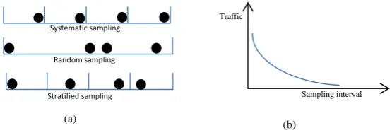
Sampling can be performed adaptively or in a non-adaptive manner. Non-adaptive sampling methods do not consider variations in traffic dynamics where measuring traffic information [6] [7]. Examples of non-adaptive sampling methods are: systematic, random and stratified. In systematic sampling, a packet is selected at a predefined fixed time interval or based on a fixed packet count. In random sampling, packets are selected at a random time intervals or based on a random packet count number. Stratified sampling combines random and stratified sampling methods by defining a fixed interval and choosing a packet randomly within the interval. Figure 1 illustrates systematic, random, and stratified sampling methods.
Figure 1. An illustration of sampling techniques: (a) Non adaptive sampling, (b) The concept of adaptive sampling [4]. Adaptive sampling can be more effective as it selects a larger number of packets when the traffic variations are higher and chooses fewer packets during reduced activities. In this study, a linguistic information processing method called fuzzy logic was used to implement adaptive sampling. Systems that their representations require complex mathematical models may be more conveniently modelled in fuzzy logic terms [8]. Fuzzy logic can be implemented in numerous ways, one of which is Fuzzy Inference System (FIS), shown in Figure 2.
Figure 2.The fuzzy inference system.
FIS has six parts, i.e. numeric inputs, fuzzification, knowledge base, inference engine, defuzzification and numeric outputs. The input is generally presented to the FIS numerically. The values are processed to determine the degrees they belong to a number of predefined membership functions called fuzzy sets. . The membership functions define the degree (extent) an input belongs to the defined fuzzy sets. Degree of membership (
) varies continuously from 0 (not a member) to1 (full member. This operation is called fuzzification of the numeric inputs. For example a traffic delay value can be fuzzified to the fuzzy sets of low_delay, average_delay and high_delay with different degrees of memberships. Therefore a value does not have to exclusively belong to a single fuzzy set as is the case in the crisp sets [9] [10]. The inference engine compares the fuzzified variable with the knowledge coded in the knowledge base to draw conclusions about the inputs. Typically the coding of the knowledge in the knowledge base is achieved by using a series of IF-THEN rules. The IF part of the rule is called the antecedent or premise while the THEN part is called the consequent or conclusion. An example of a rule is: IF delay is very_high THEN QoS is poor. The output from the inference engine is defizzified to produce numeric values by using a number of output membership functions.
FIS has been previously used for adaptive sampling of computer network traffic [11] [12]. The main differences between this study and those reported in [11][12] are that in this study the traffic
(a)
Systematic sampling
Random sampling
Stratified sampling
Traffic
Sampling interval
(b)
Numeric Inputs
Knowledge base
Inference Engine
was modelled using linear regression prior to using the FIS and a physical rather than a simulated network was used.
Regression analysis is a technique for exploring the relationship between dependent and independent variables [13] [14]. Regression can be linear or nonlinear but linear regression is more commonly used for predictive and for analysis tasks and is the type used in this study. Regression models has been used for future sensors network readings, allowing network processes to be predicted based on the current captured data or based on the nearest network node [15]. This led to a reduction in the amount of transmitted data packets.
In our study, the output from the regression model was interpreted using fuzzy logic. The main contributions of this study is that a novel adaptive sampling technique that can simultaneously sample three main traffic parameters, i.e. delay, jitter and percentage packet loss ratio, in a physical computer network is developed. The method can quantify overall network QoS for multimedia networks.
2. Materials and Methods
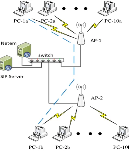
The developed adaptive sampling method was evaluated using a wireless computer network (shown in Figure 3) set up in a network research laboratory with an area of 4 m × 6 m. The aim was to explore how well the adaptively sampled traffic represents the original traffic for QoS assessment.
AP-1
AP-2
switch
SIP Server
PC-1b PC-2b PC-10b
PC-1a PC-2a PC-10a
Netem
Figure 3. The network topology used in the study.
The network consisted of two Cisco© AIR-AP1852E access points (APs) operating using the
IEEE 802.11ac/n Wi-Fi standard. Cisco© APs contain four external dual-band antennas. Cisco©
catalyst 3560-CX switch connected the two APs with Session Initiation Protocol (SIP) server via 1 Giga bits per second (Gbps) wired links. The specifications of the Personal computers (PCs) used in the study were: Intel© Core i7-3770 processor, 3.40 GHz, 16 GB DDR3 RAM, Microsoft Windows© 7
Enterprise SP1 64 bits, for 802.11ac Linksys© AC1200 Dual-Band wireless adaptor. There was no
encryption activated between the APs and the PCs' wireless adapters. The wireless devices were close to each other, the transmission power was kept as 30 mW (15 dBm) [16].
used Real Time Transport protocol (RTP). X-Lite Softphones software ran over the Microsoft Windows© operating system providing SIP VoIP, using G711a coder-decoder (CODEC), RTP was
used with a packet size of 160 bytes. Queuing mechanism for all scenarios was First-In-First-Out (FIFO) chosen for its simplicity and queue size was 50 packets.
Wireshark [17] network monitoring tool was used to capture traffic packets based on the protocol type such as User Datagram Protocol (UDP), TCP, Real Time Control Protocol (RTCP), Real Time Protocol (RTP) and SIP. Wireshark was installed on two computers, PC-1a connected to AP-1 and the other on PC-1b connected to AP-2. These captured the packets that were used to determine end-to--end delay, jitter and percentage packet loss ratio. The operation established point-to-point protocol (PPP) links between the PCs that connected to AP-1 and PCs that connected to AP-2. First PC-1a to PC-1b PPP link was established. Traffic was sent over this PPP link that included high definition (HD) video, VoIP and TCP traffic. The resulting traffic packets were captured using the Wireshark.
As a large amount of packets were sent, sampling was needed to evaluate QoS. An adaptive sampling technique was developed to select packets that best represented the original traffic.
Netem is a network emulation tools used to emulate packet loss, delay and jitter [18]. In this study this software was used to alter delay, jitter and percentage packet loss ratio between the communicating PC-1a and PC-1b. Netem allowed a more realistic traffic to be established with regard to transmission rate, delay and packet loss.
2.1. Network traffic parameters
The Wireshark network monitoring captured RTP packets (installed on the two the PCs) were sorted using their sequence numbers to determine end-to-end delay, jitter and percentage packet loss ratio as below [19][20][21]:
End to end delay was determined for each packet. For the ith packet, delay (Di) was calculated
by subtracting the arrival time for the packet (𝑅𝑖) from the sent time (𝑆𝑖) as indicated by Equation (1),
𝐷𝑖 = 𝑅𝑖− 𝑆𝑖 (1)
The magnitude of jitter (Ji) was measured by determining the difference between the current
packet delay (𝐷𝑖) and the delay for the previous packet (𝐷𝑖−1) as in Equation (2),
𝐽𝑖= 𝑚𝑎𝑔𝑛𝑖𝑡𝑢𝑑𝑒 (𝐷𝑖− 𝐷𝑖−1) (2)
The percentage packet loss ratio (%PLRi) was measured by determining the total number of
received packets (∑ 𝑅𝑖 (𝑡)) and the total number of sent packets (∑ 𝑆𝑖 (𝑡)) at a given time (t) as illustrated in Equation (3),
%𝑃𝐿𝑅𝑖(𝑡) = (1 −
∑ 𝑅𝑖 (𝑡)
∑ 𝑆𝑖(𝑡)) × 100 (3)
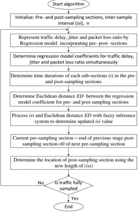
Once the traffic parameters (delay, jitter and percentage packet loss ratio) were obtained, they were processed by the developed adaptive sampling method. The method used linear regression to model the traffic and the output from the model was interpreted by the fuzzy inference system (FIS) to dynamically adjust the number of packets selected for QoS assessment. The algorithm’s
operation is illustrated in the flow chart shown in Figure 4. The elements of the algorithm are:
• Pre- and post-sampling section: These intervals contain the traffic that needs to be sampled. The duration of these intervals are kept fixed (predefined) and do not change during sampling process.
• Inter-section interval (isi): This interval is between the pre- and post-sampling sections. Its duration is adaptively updated by the FIS.
• Euclidean distance (ED): ED was used to quantify the amount of traffic variation between the pre- and post-sampling sections.
• Fuzzy inference system: FIS was used to update the duration of the isi based on its current value and the ED measures.
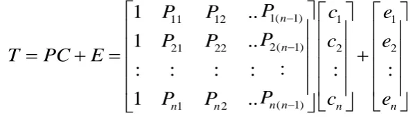
The regression model provided the traffic coefficients for the pre- and post-sampling sections. The traffic parameters delay, jitter and percentage packet loss ratio were considered as the independent variables representing p values in regression Equation (4), the sampling section was divided into sub-sections (s1, s2,...sn), each sub-section containing (n-1) packets as shown in Figure 5
where the traffic values of each sub-section was represented by a row of matrix P and the associated time period of every sub-section represented by the vector T as indicated in Equation (4).
Start algorithm
Start algorithm
Initialise: Pre- and post-sampling sections, Inter-sample interval (isi), n
Initialise: Pre- and post-sampling sections, Inter-sample interval (isi), n
Represent traffic delay, jitter and packet loss ratio by Regression model incorporating pre- post- sections
Represent traffic delay, jitter and packet loss ratio by Regression model incorporating pre- post- sections
Current pre-sampling section = end of previous stage post-sampling section+t0 of next pre-post-sampling section
Current pre-sampling section = end of previous stage post-sampling section+t0 of next pre-post-sampling section
Determine the location of post-sampling section using the new length of (isi)
Determine the location of post-sampling section using the new length of (isi)
End
End
Determine Euclidean distance ED between the regression model coefficient for pre- and post sampling sections
Determine Euclidean distance ED between the regression model coefficient for pre- and post sampling sections
Is traffic fully sampled
Is traffic fully sampled No
Yes
Process isi and Euclidean distance ED with fuzzy inference system to determine updated isi value
Process isi and Euclidean distance ED with fuzzy inference system to determine updated isi value
Determine time durations of each sub-sections (t)in the pre- and psot-sampling sections
Determine time durations of each sub-sections (t)in the pre- and psot-sampling sections
Determine regression model coefficients for traffic delay, jitter and packet loss ratio simultaneously
Determine regression model coefficients for traffic delay, jitter and packet loss ratio simultaneously
Figure 4. The flow chart of the adaptive sampling algorithm.
Tr
af
fic
Time
Pre-sampling section Post-sampling section
inter-sampling interval
(isi)
{
S1pre
{ {
S2pre S(n)pre{
S1post S{
2post S(n)post{
In this study, n was chosen as 4 resulting in a 4×4 traffic matrix (P). This generated three sub-sections: S1pre, S2pre, S3pre and S4pre for pre-sampling section and S1post, S2post, S3post and S4post for post-sampling. Each subsection contained 3 data packets. This was repeated for the pre- and sampling sections. The general representation of the traffic matrices for pre- and post-sampling section is shown in Equation 4.
1( 1)
11 12 1 1
2( 1)
21 22 2 2
( 1) 1 2
1
..
1
..
:
:
:
:
:
:
:
1
..
n n n nn n n n
P
P
P
c
e
P
P
P
c
e
T
PC
E
P
P
P
c
e
(4)The time durations associated with each sub-sections (s1, s2,...sn) were represented by t1, t2 …
tn. These durations were measured by subtracting the arrival time of the last packet from the arrival
time of first packet in the corresponding sub-section. The regression coefficients c1, c2, … cn were determined by Equation 5.
𝐶 = 𝑃−1𝑇 (5)
The amount of variation in traffic associated with pre- and post- sampling sections was quantified by comparing their respective regression model coefficients using the Euclidean distance as shown in Equation 6.
𝐸𝑢𝑐𝑙𝑖𝑑𝑒𝑎𝑛 𝑑𝑖𝑠𝑡𝑎𝑛𝑐𝑒
= √(𝑐1𝑝𝑟𝑒− 𝑐1𝑝𝑜𝑠𝑡)2+ (𝑐2𝑝𝑟𝑒− 𝑐2𝑝𝑜𝑠𝑡)2+ ⋯ (𝑐(𝑛)𝑝𝑟𝑒− 𝑐(𝑛)𝑝𝑜𝑠𝑡)2 (6)
FIS received the current duration of inter-sampling interval (isi) and the Euclidean distance (ED) and then determined the updated value of isi duration as shown in Figure 6.
Euclidean distance of delay ED_D inter-sampling interval (isi)
Updated inter-sampling interval
(isi)
Euclidean distance of jitter ED_J Euclidean distance of PL ED_PL
Fuzzy inference system
FIS
Figure 6. Fuzzy system to update isi duration.
The Mamdani type FIS was used to adaptively adjust the length of isi. Four inputs were fed into the FIS. They were the current inter-sampling interval, network parameters delay, jitter and percentage packet loss ratio. The inputs and the output were fuzzified using the Gaussian membership functions that has a concise notation and is smooth. The Gaussian membership function is represented by formula is expressed in (7) where ci and σi are the mean and standard
deviation of the ith fuzzy set Ai [2].
2
2
( )
( ) exp
2 i i A i c x x
(7)
Tables (I) and (II) show the mean and standard deviations of the Gaussian membership functions for the fuzzy input sests (i.e. delay, jitter, %PLR, and current isi) and fuzzy output sets (i.e. updated isi) respectively.
Table I. Mean and standard deviation of the Gaussian fuzzy sets for inputs (Euclidian delay, Euclidian jitter and Euclidian %PLR).
Membership functions (Mean, Standard deviation (Std)) for ED delay, ED jitter , ED of %PLR
Very low 0.1, 0
Low 0.1, 0.25
Medium 0.1, 0.5
High 0.1, 0.75
Very high 0.1, 1
Table II. Mean standard deviation of the Gaussian fuzzy sets for inter-sample interval difference and output updated inter-sample interval.
Membership functions
current isi
Membership functions updated isi
(Mean, Standard deviation) for Current and
updated isi
Very small Decrease low (DL) 10, 0
Small Decrease High (DH) 10, 25
Medium No change (NC) 10, 50
Large Increase low (IL) 10, 75
Very large Increase high (IH) 10, 100
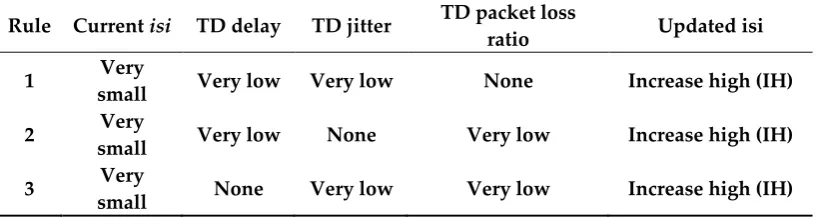
The relationship between the inputs, current isi duration and the Euclidean distance with the output (i.e. updated isi duration) was represented by twenty rules as shown in Table III.
Table III. Rules included in the FIS knowledge base.
Rule Current isi TD delay TD jitter TD packet loss
ratio Updated isi 1 Very
small Very low Very low None Increase high (IH) 2 Very
small Very low None Very low Increase high (IH) 3 Very
4 None Very low Very low Very low Increase high (IH)
5 None Low Low Low Increase low (IL)
6 Small None Low Low Increase low (IL)
7 Small Low None Low Increase low (IL)
8 Small Low Low None Increase low (IL)
9 Medium Medium Medium None No change (NC)
10 Medium Medium None Medium No change (NC)
11 Medium None Medium Medium No change (NC)
12 None Medium Medium Medium No change (NC)
13 None High High High Decrease low (DL)
14 Large None High High Decrease low (DL)
15 Large High None High Decrease low (DL)
16 Large High High None Decrease low (DL)
17 None Very
high
Very
high Very high Decrease low (DH) 18 Very large None Very
high Very high Decrease low (DH) 19 Very large Very
high None Very high
Decrease High (DH) 20 Very large Very
high
Very
high None
Decrease High (DH)
The inputs to the FIS, i.e. the ED and current inter-sample interval were fuzzuified using three membership functions. The ED was represented Low, Medium and High fuzzy sets and the current inter-sample interval (isi) was represented by Small, Medium and Large fuzzy sets. The output was defizzified by four membership functions, represented as IL (low increase), NC (no change), DL (low decrease), and DH (high decrease). These membership functions are shown in Figure 7.
(c) (d)
(e)
Figure 7. Membership functions for (a-c) the Euclidean distance sets for delay, jitter and percentage packet loss ratio. (d) inter-sampling interval (e) the updated inter-sampling interval.
To evaluate the effectiveness of the developed adaptive sampling method, comparisons of the original traffic's data packets and its sampled versions were carried out. Comparisons of mean and standard deviation of the sampled packets to its original populations may not be enough to evaluate the accuracy of sampled version in terms of demonstrating the original population as they can be obscured by outliers [22] [23]. Therefore additional evaluations were used to assess the efficiency of the developed sampling approach. The bias indicates how far the mean of the sampled data lies from the mean of its original population [23]. Bias is the average of difference of all samples of the same size. The bias was calculated as in equation (10).
Ni
i
M
M
N
Bias
1
1
(10)
Where N is the number of simulation run, Mi and M are the means of the traffic parameters for the
original data and its sampled population.
Relative Standard Error (RSE) is another parameter that can be used to assess the accuracy and efficiency of the technique, RSE examines the reliability of sampling [5]. RSE is defined as a percentage and can be defined as the standard error of the sample (SE) divided by the sample size (n) as in equation (11).
100
n
SE
RSE
(11)where n is sample size, SE is standard error values of the original and sampled data population.
N N
N N
N
a
x
a
x
a
x
a
x
a
x
f
(
)
0
1 1
2 2
...
1
(12)Polynomial curve fitting function measures a least squares polynomial for a given data set of (x) and generates the coefficients of the polynomial which can be used to illustrate a curve to fit the data according to the specified degree (N).The degree of a polynomial is equal to the maximum value of the exponents (N), [a0…aN] is a set of polynomial coefficients. The polynomial evaluation
function examines a polynomial for a x values and then produces a curve to fit the data based on the coefficients that were found using the curve fitting function [24] [26].
Sampling fraction is the proportion of a population that will be counted. Sampling fraction is the ratio of the sampled size (n) divided by the population size. In this study, the curve fitting results have been marked by red color to demonstrate original and sampled data trends.
3. Results and Discussion
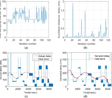
The traffic consisting of packets for different applications were captured and their parameters, i.e. delay, jitter and percentage packet loss ratio were determined using Equations 1-3. The simulation duration was up to three minutes. The linear regression Equations 4 and 5 were used to model the traffic. The Euclidean distance ED shown in Equation 6 was used to quantify the variation in the behavior of the traffic associated with the pre- and post-sampling sections. The FIS output indicated the updated isi duration for each iteration, based on the values of the FIS inputs and the fuzzy rules. As an example, Figure 8(a) indicates the adaptive updating of isi based on the variations in packet delay. Figure 8(b) indicates the manner the Euclidean distance, the variation of Euclidean distances of delay, jitter and packet loss ratio affect isi changes. When traffic variations were large, isi decreased and vice versus. Figure 8(c) shows the original delay and its trend and Figure 8(d) indicates the sampled delay and its trend. The trends for the original delay and its sampled version are close. In Figures 8c-e the curve fitting method has been used for both original and sampled version of the traffic parameters, the fitted curve shown in red indicates the data trend for original population and sampled version. The trend of the sampled version using the adaptive sampling technique represents the original data closely.
(a) (b)
(c) (d)
(a) (b)
(c) (d)
(e) (f)
Figure 9. Typical results obtained from the developed adaptive technique: (a) measured Euclidean distance for jitter, (b) measured Euclidean distance for packet loss (c) original traffic jitter, (d) sampled traffic percentage jitter (e) original traffic packet loss ratio (f) sampled traffic packet loss ratio.
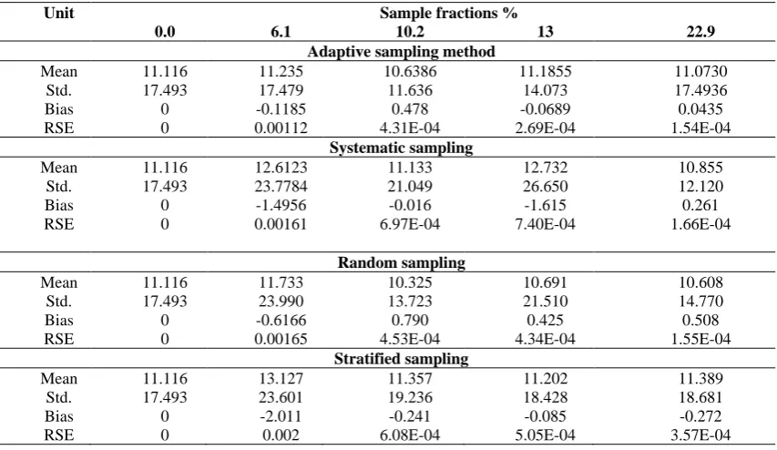
Table IV provides a summary of delay sampling results for the original traffic (0% sample fraction) and a number of different sample fractions for the adaptive and non-adaptive sampling methods of systematic, random and stratified. Similar information is provided for jitter and %PLR in Tables V and VI. To compare the developed adaptive sampling and non-adaptive sampling methods, the bias and relative standard errors (RSE) were determined. They indicated that the developed adaptive method has the lowest relative error and bias values in most of sample fractions as compared as compared with the non-adaptive methods, signifying an improved performance.
ms, and 139 ms) respectively. These indicate s that the delay sampled versions by adaptive sampling technique represented the original delay more accurately and effectively.
Table IV. Measurement results of delay using different sampling methods: adaptive, systematic, random and stratified.
Unit Sample fractions %
0 6.1 10.2 13 22.9 Adaptive sampling method
Mean 1.46E+02 1.47E+02 1.47E+02 1.47E+02 1.47E+02
Std. 1.41E+02 1.41E+02 1.41E+02 1.42E+02 1.41E+02
Bias 0 0.875 0.683 0.067 -0.262
RSE 0 0.0090 0.0040 0.0030 0.0011
Systematic sampling
Mean 1.47E+02 1.45E+02 1.46E+02 1.48E+02 1.43E+02
Std. 1.41E+02 1.46E+02 1.42E+02 1.41E+02 1.38E+02
Bias 0 1.9740 0.725 -1.279 3.960
RSE 0 0.0099 0.0052 0.0038 0.0019
Random sampling
Mean 1.47E+02 1.76E+02 1.57E+02 1.49E+02 1.50E+02
Std. 1.41E+02 1.65E+02 1.52E+02 1.49E+02 1.42E+02
Bias 0 -28.551 -9.741 -1.401 -2.432
RSE 0 0.0113 0.0050 0.0029 0.0014
Stratified sampling
Mean 1.47E+02 1.46E+02 1.50E+02 1.50E+02 1.49E+02
Std. 1.41E+02 1.43E+02 1.49E+02 1.42E+02 1.39E+02
Bias 0 1.0932 -2.74034 -2.9770 -2.1844
RSE 0 0.0127 0.0046 0.00389 0.00265
Std: standard deviation
The results indicate similar trend for jitter as indicated in Table V. The mean and standard deviation of original jitter population were 11.116 ms and 17.493 ms respectively, whereas the sampled jitter population obtained from the adaptive sampling method had the mean of 11.073 ms and standard deviation of 17.494 ms, respectively at 22.9% sample fraction. However, the mean and standard deviation of original data population of sampled jitter using systematic, random and stratified sampling were (10.855 ms, 10.608 ms, and 11.389 ms) and (12.120 ms, 14.770 ms and 18.681 ms) respectively. This indicates that the jitter for sampled versions using the adaptive sampling technique represented the original jitter more accurately.
Table V. Measurement results of jitter using different sampling methods: adaptive, systematic, random and stratified.
Unit Sample fractions %
0.0 6.1 10.2 13 22.9 Adaptive sampling method
Mean 11.116 11.235 10.6386 11.1855 11.0730
Std. 17.493 17.479 11.636 14.073 17.4936
Bias 0 -0.1185 0.478 -0.0689 0.0435
RSE 0 0.00112 4.31E-04 2.69E-04 1.54E-04
Systematic sampling
Mean 11.116 12.6123 11.133 12.732 10.855
Std. 17.493 23.7784 21.049 26.650 12.120
Bias 0 -1.4956 -0.016 -1.615 0.261
RSE 0 0.00161 6.97E-04 7.40E-04 1.66E-04
Random sampling
Mean 11.116 11.733 10.325 10.691 10.608
Std. 17.493 23.990 13.723 21.510 14.770
Bias 0 -0.6166 0.790 0.425 0.508
RSE 0 0.00165 4.53E-04 4.34E-04 1.55E-04
Stratified sampling
Mean 11.116 13.127 11.357 11.202 11.389
Std. 17.493 23.601 19.236 18.428 18.681
Bias 0 -2.011 -0.241 -0.085 -0.272
Table VI indicates a similar trend for %PLR. The mean and standard deviation of original %PLR population were 0.0356 mc and 0.0291 ms respectively, whereas the sampled %PLR population obtained from the adaptive sampling method had the mean of 0.035 ms and standard deviation of 0.029 ms, respectively at 22.9% sample fraction. However, the mean and standard deviation of original data population of sampled %PLR using systematic, random and stratified sampling were (0.035 ms, 0.035 ms, and 0.036 ms) and (0.029 ms, 0.0294 ms, and 0.0286 ms) respectively. This specifies that the %PLR sampled versions by adaptive sampling technique represented the original PLR more accurately and effectively.
Table VI. Measurement results of packet loss ratio using different sampling methods: adaptive, systematic, random and stratified.
Unit Sample fractions %
0.0 6.1 10.2 13 22.9 Adaptive sampling method
Mean 0.0356 0.035 0.034 0.036 0.035
Std. 0.0291 0.0292 0.0290 0.029 0.029
Bias 0 6.23E-06 0.0016 -5.96E-04 -7.22E-05
RSE 0 1.88E-06 3.05E-07 5.93E-07 2.08E-07
Systematic sampling
Mean 0.0356 0.037 0.035 0.035 0.035
Std. 0.0291 0.029 0.0290 0.028 0.029
Bias 0 -0.0014 5.20E-04 7.95E-06 -2.72E-04
RSE 0 2.06E-06 9.62E-07 8.05E-07 3.99E-07
Random sampling
Mean 0.0356 0.035 0.0343 0.034 0.035
Std. 0.0291 0.029 0.027877 0.028954 0.029492
Bias 0 1.65E-05 0.0013 8.07E-04 -2.90E-04
RSE 0 1.98E-06 1.03E-06 7.94E-07 3.30E-07
Stratified sampling
Mean 0.0356 0.034 0.035 0.037 0.036
Std. 0.0291 0.028 0.029 0.029 0.0286
Bias 0 0.0013 1.03E-06 -0.0014 -6.45E-04
RSE 0 2.55E-06 9.35E-07 8.13E-07 5.47E-07
Figures 10a-c show respectively comparisons of the bias of sampled delay, jitter and %PLR for different sample fractions using the proposed adaptive sampling method and non-adaptive sampling methods of systematic, random and stratified. The results indicate that the bias was decreased and became closer to zero for all sampling methods when the sample size increased. The results indicate that the proposed adaptive sampling method has a lower bias as compared with systematic, stratified, and random sampling approaches. For example, at 22.9% sample fraction, the bias of sampled delay was -0.262, while the bias values by systematic, random and stratified sampling were 3.960, -2.432, and -2.1844respectively. When the sample fraction was the lowest value, i.e. 6.1%, the least biasness was by the developed adaptive method with 0.875, followed by stratified sampling method with 1.093, then systematic methods with 1.974, and the highest biasness was for random method at -28.55.
(a) (b)
(c)
Figure 10. Comparisons of biasness of (a) delay, (b) jitter and (c) %PLR between developed technique and non-adaptive methods.
(a) (b)
(c)
Figure 11. Comparisons of RSE of (a) delay, (b) jitter and (c) PLR between developed technique and non-adaptive methods.
4. Conclusions
A novel adaptive technique that samples computer network traffic has been developed and its performance has been compared with the non-adaptive sampling methods of random, stratified and systematic. The developed method adaptively adjusted a section called inter sampling interval resulting in an increase in sampling when the traffic variations were greater and vice versus. The developed adaptive sampling represented the original traffic more closely than the non-adaptive sampling. The developed adaptive method successfully applied to a physical computer network and showed a better performance. The developed adaptive sampling method can be valuable for evaluating multimedia network performance.
Acknowledgments: The authors are grateful to receive Sheffield Hallam University Vice Chancellor's PhD Studentship funding that allowed this work to be carried out.
References
[1]W. Robitza, A. Ahmad, P.A. Kara, L. Atzori, M. G. Martini, Al. Raake and L. Sun, "Challenges of future multimedia QoE monitoring for internet service providers," Multimed Tools Appl. (2017), DOI 10.1007/s11042-017-4870-z, Online, https://pearl.plymouth.ac.uk/bitstream/handle/10026.1/9869/Challenges_of_future.pdf?sequence=1.
[2]M.A.V. Rodíguez, E.C. Muñoz, "Review of quality of service (QoS) mechanisms over IP multimedia subsystems (IMS)," Ingeníeria y Desarrollo Universidad del Norte, 35(1) (2017), 262-281.
[3]R. Lin, O. Li, Q. Li and K. Dai, "Exploring adaptive packet-sampling measurements for multimedia traffic classification,", Journal of Communication, 9(12) (2014), 971-979.S. Fernandes, C. Kamienski, J. Kelner, D. Mariz and D. Sadok, "A stratified traffic sampling methodology for seeing the big picture,", Computer Networks, 52, 2677-2689, 2008.
[4]A. Salama, R. Saatchi, and D. Burke, ''Quality of Service Evaluation and Assessment Methods in Wireless Networks,'' In: The 4th International Conference on Information and Communication Technologies for Disaster Management, Munster, Germany, 11-13 December 2017.
[5]R. Serral-Gracià, A. Cabellos-Aparicio, and J. Domingo-Pascual, ''Network performance assessment using adaptive traffic sampling,'' A. Das et al. (Eds.): Networking, LNCS 4982, 252–263, 2008.
[6]J. M. C. Silva, C. Paulo and R. L. Solange, "Inside packet sampling techniques: exploring modularity to enhance network measurements," International Journal of Communication Systems 30(6), 2017.
[7]R. Bělohlávek, J. K. George, and J. W. Dauben, ''Fuzzy logic and mathematics: a historical perspective,'' Oxford University Press, 2017.
[9]T. J. Ross, "Fuzzy logic with engineering applications,", Fourth Edition, Wiley, 2017.
[10]A. Dogman, R. Saatchi, S. Al-Khayatt, and H. Nwaizu, ''Adaptive statistical sampling of voip traffic in wlan and wired networks using fuzzy inference system,'' 2011 7th International Wireless Communications and Mobile Computing Conference, 1731-1736, 2011.
[11] A. Dogman, R. Saatchi, S. Al-Khayatt. ''An adaptive statistical sampling technique for computer network traffic,'' IEEE Explore, 7th International Symposium on Communication Systems Networks and Digital Signal Processing (CSNDSP) , 479-483, 2010. [12] J. Fan, Y. Liao, and H. Liu, ''An overview of the estimation of large covariance and precision matrices,'' The Econometrics Journal,
19(1), C1-C32 [4], 2016.
[13] J. J. Faraway, ''Extending the linear model with R: generalized linear, mixed effects and nonparametric regression models,'' (volume 124). CRC press, 2016.
[14] B. Zhang, Y. Liu, J. He and Z. Zou, ''An energy efficient sampling method through joint linear regression and compressive sensing,'' In Intelligent Control and Information Processing (ICICIP), 2013 Fourth International Conference on, IEEE, 447-450, 2013.
[15] J. A. R. P. de Carvalho, H. Veiga, C. F. C. F. Ribeiro and A.D. Reis. "Performance evaluation of IEEE 802.11 a, g laboratory open point-to-multipoint links," Proceedings of the World Congress on Engineering. vol.I, , WCE July 1-3, London, U.K., 2015. [16] C. Sanders, ''Practical packet analysis: Using Wireshark to solve real-world network problems,'' No Starch Press, 2017.
[17] D. Yohannes and M. Dilip, "Effect of delay, packet loss, packet duplication and packet reordering on voice communication quality over WLAN," Technia 8(2), 1071, (2016)
[18] A. Salama, R. Saatchi and D. Burke, ''Adaptive sampling technique for computer network traffic parameters using a combination of fuzzy system and regression model,'' In: 2017 4th International Conference on Mathematics and Computers in Science in Industry, MCSI 2017, Island, Greece, August. IEEE. 24-26, 2017.
[19] A. Salama, R. Saatchi and D. Burke, ''Adaptive sampling technique using regression modelling and fuzzy inference system for network traffic,'' In: CUDD, Peter and De Witte, Luc, (eds.) Harnessing the power of technology to improve lives. Studies in Health Technology and Informatics (242). IOS Press, 592-599, 2017.
[20] A. Salama, R. Saatchi, and D. Burke, "Adaptive sampling for QoS traffic parameters using fuzzy system and regression model," Mathematical Models and Methods in Applied Sciences, 11, 212-220, 2017.
[21] A. Dogman, R. Saatchi, S. Al-Khayatt, and H. Nwaizu, ''Adaptive statistical sampling of VoIP traffic in WLAN and wired networks using fuzzy inference system,'' 2011 7th International Wireless Communications and Mobile Computing Conference, 1731-1736, 2011.
[22] T. Zseby, ''Comparison of sampling methods for non-intrusive SLA validation,'' In Proceedings of the Second Workshop on End-to-End Monitoring Techniques and Services (E2EMon), 2004.
[23] X. Wan, Y. Li, C. Xia, M. Wu, J. Liang, and N. Wang, "A T-wave alternans assessment method based on least squares curve fitting technique," Measurement 86, , 93-100, 2016.
[24] V. Guruswami and D. Zuckerman, "Robust Fourier and polynomial curve fitting," Foundations of Computer Science (FOCS), 2016 IEEE 57th Annual Symposium on. IEEE, 2016.