Grid multi-category response logistic models

(1)

R E S E A R C H A R T I C L E

Open Access

Grid multi-category response logistic models

Yuan Wu

1*

, Xiaoqian Jiang

2

, Shuang Wang

2

, Wenchao Jiang

3

, Pinghao Li

3

and Lucila Ohno-Machado

2

Abstract

Background:Multi-category response models are very important complements to binary logistic models in medical decision-making. Decomposing model construction by aggregating computation developed at different sites is necessary when data cannot be moved outside institutions due to privacy or other concerns. Such decomposition makes it possible to conduct grid computing to protect the privacy of individual observations.

Methods:This paper proposes two grid multi-category response models for ordinal and multinomial logistic regressions. Grid computation to test model assumptions is also developed for these two types of models. In addition, we present grid methods for goodness-of-fit assessment and for classification performance evaluation.

Results:Simulation results show that the grid models produce the same results as those obtained from corresponding centralized models, demonstrating that it is possible to build models using multi-center data without losing accuracy or transmitting observation-level data. Two real data sets are used to evaluate the performance of our proposed grid models.

Conclusions:The grid fitting method offers a practical solution for resolving privacy and other issues caused by pooling all data in a central site. The proposed method is applicable for various likelihood estimation problems, including other generalized linear models.

Keywords:Grid MLE, Ordinal logistic model, Multinomial logistic model

Background

In biomedical research, data sharing plays an important role in accelerating scientific discoveries. For example, networks based on information from electronic health record (EHR) [1,2] have been established for this pur-pose. However, due to privacy concerns, patient-level data cannot always be exchanged across different institu-tions. In these circumstances grid computing, which avoids sharing patient level data among multiple institu-tions, can be used to build a global model.

For example, logistic regression models have been used in a variety of clinical applications, such as scoring candi-dates for liver transplant using the Model for End-stage Liver Disease [3], producing estimates related to myocar-dial infarction diagnosis [4], and detecting suspicious ac-cesses to electronic health records [5]. These scenarios, in their classical setups, have difficulties in handling multi-center data, as the training phase requires accessing the entire dataset.

Our previous work [6] and [7] proposed privacy-preserving models through the aggregation of non-sensitive intermediary results (i.e., gradient and Hessian matrix for the log-likelihood function), but the model only deals with binary models. Response variables with more than two categorical values occur very often in medical models. For example, cancer progress is often categorized into 4 or 5 phases. One simple method to deal with multiple responses is to fit binary logistic fit-ting for each pair of these multiple categories. However, this approach is very inconvenient and the performance of each binary logistic model might be degraded when sample size is insufficient. Some researchers extended the binary logistic model to handle multi-category re-sponse problems. Among existing approaches, ordinal logistic [8] and multinomial logistic [9] are the two most popular multi-category response logistic models for or-dinal and nominal responses, respectively. Both methods are widely used to fit data with multi-category response. However, methods for binary model fitting assessment may not be applicable to multi-category problems. Hosmer and Lemeshow [9] introduced novel methods to evaluate the goodness-of-fit of multi-category logistic models. The Area

* Correspondence:[email protected] 1

Department of Biostatistics & Bioinformatics, Duke University, Durham, NC 27708, USA

Full list of author information is available at the end of the article

(2)

Under the ROC Curve (AUC) [10] is an important measure in checking classification performance of binary outcome models. Hand and Till [11] generalized the original AUC measure to deal with classification methods for multi-category outcome cases. The AUC for binary logistic re-gression is given by

^

Að1j0Þ ¼R−½ðn1þ1Þn1=2 n1n2 ;

where n1, n2 are the number of observations with Y=1 and withY=0,Ris the rank sum based on the predicted probability of Y= 1 for observations with Y= 1 among all observations. Van Calsteret. al.[12] described several AUC score estimation methods for the ordinal logistic model, one of which is to use the mean of AUC scores fromK−1 binary logistic regression estimations to serve as the AUC score for ordinal logistic model. Hand and Till [11] defined Â(k1|k2) in the same way for observa-tions with Y∈{k1,k2} and proposed a generalized AUC for multinomial logistic model as _{K K}_ð2₋₁_ÞX_k_1<_k

2

^

A k1k2Þ þA k^ð 1jk2Þ=2

for 1≤k1,k2≤K. Yang and Carlin [13] generalized the ROC curve to a surface and used the volume under the ROC surface (VUC) to measure the accuracy of a diagnostic test based on multi-category response models. Dreiseitl et. al. [14] proposed to use a three-way ROC curve analysis for the same goal. Van Calsteret. al.[12] suggested an ordinal c-index measurement (ORC) and discussed the relation-ship between the new measurement with VUC and other measurements based on assessing pairs of cases.

In this article, we introduce grid ordinal and multi-nomial logistic models to handle multi-center modeling of multi-category response, including model assumption checking. We also propose to use the grid AUC score to evaluate the added value of the grid model fitting when compared to models fitted by separate sub-datasets. The remainder of this article is organized as follows. The sec-ond Section briefly reviews ordinal logistic [8] and multinomial logistic [9] models and their model as-sumptions, and also discusses model coefficient esti-mation methods for both models and the statistical test for checking the ordinal logistic assumption. The third Section discusses grid maximum likelihood esti-mation and grid computing for the ordinal logistic model assumption test statistics. The fourth Section provides technical details for grid model fitting assess-ment. The fifth Section elaborates on grid AUC score computing. The sixth Section describes simulation studies to evaluate the theoretical results. The seventh Section carries out additional experiments on two real datasets to demonstrate our proposed methods. The eighth Section discusses the generalization of the pro-posed grid models and the limitations of this work.

Methods

Ordinal and multinomial logistic models

Before we introduce our method we first introduce both ordinal and multinomial logistic models in a few more detail. In terms of how to split response categories, many ordinal logistic models have been studied. How-ever, in this article, we only focus on the proportional odds logistic model to deal with multi-category prob-lems. The proposed method will be extended to other multi-category logistic regression models in the future. Suppose responseYcould take values 1,⋯,K(forK cat-egories) with K≥3. There are m features in the model and n observations. The predictor matrix can be expressed asXT= (x1,⋯,xn) with xTi ¼xi;1;⋯;xi;mfor

1≤i≤n. Let’s define p(w,i)≜Pr(Y≤w|xi) and assume 1≤i≤nand 1≤w≤K−1. The ordinal logistic regression [8] can be defined as

p wð ;iÞ ¼ eαwþβ

T_x i

1þeαwþβTxi; ð1Þ

With parameters βT= (b1,⋯,bm). The conditional likelihood function is given by

L¼Πn i¼1

n

pð Þ1;i I½yi¼1ΠK−1

w¼2½p wð ;iÞ−p wð −1;iÞ

I_½_yi_¼_w

⋅½1−p Kð −1;iÞI½yi¼Ko_;

ð2Þ

where I½yi¼w is the indicator function, with value of 1 if yi=w and 0 otherwise. Let θ = (α1, α2, ⋯, αK−1, βT)T, the log-likelihood function for the proportional odds lo-gistic model be denoted aslO(θ). The maximum likelihood estimation (MLE)^θ forlO(θ) is usually computed using the Newton method for efficiency. The variance-covariance matrix for^θis estimated by− ∂2_l

Oð Þθ =

½ ∂θ∂θT_j_θ_^−1

. Equation (1) assumes that the non-intercept model co-efficientsβremain the same for 1≤w≤K−1. Usually, a justification for the model assumption is needed when fitting ordinal logistic model. This assumption is called proportional odds assumption [15]. The score test is a common way to test the proportional odds assumption. To perform the score test, we first introduce the gener-alized ordered logit model [16], which is a generalization of the ordinal logistic model as it allows non-intercept model coefficients to be different. The generalized or-dered logit model is given by

T wxi

1þeαwþβTwxi; ð3Þ

with βTw¼bw;1;⋯;bw;m for 1≤i≤n and 1≤w≤K−1.

Let us denote ψ¼ α1;βT1;⋯;α2;βTK−1

T

(3)

log-likelihood function for this generalized model, lG(ψ), is obtained by combining (3) and (2). From its definition, we see that the generalized ordered logistic model re-quires more parameters than the proportional odds model. Hence, model fitting for small sample size data is a big concern for the generalized ordered logistic model. To check the proportional odds assumption, we need to test whether β1=⋯=βK−1. As mentioned previously, suppose ^θ¼ α^1;⋯;^αK−1;^β

n o

is the MLE for lO(θ). Let ψe¼ α^1;β^;⋯;αK−1;β^

n o

.The score test statistic is

To¼ ∂lGð Þψ ∂ψ jψe

# T

"

−∂_∂2_ψlG_∂ð Þ_ψψ_T jψe #

−1

"

∂lGð Þψ ∂ψ jψe

# : "

ð4Þ

Under the null hypothesisβ1=⋯=βK−1,To asymptot-ically followsχ2

m Kð −2Þ.

The multinomial logistic model is mainly dealing with a nominal response with unordered categories. It does not require the proportional odds assumption. Using the multinomial model on ordered data disregards the inher-ent information in the ordering of the response categor-ies and is not, in general, recommended. Suppose the response variable and predictors are the same as de-scribed in the proportional odds model except that the proportional odds assumption does not hold. Let’s de-notep w~ð ;iÞ≜Pr Yð ¼w xj iÞ.In multinomial logistic model for 1≤i≤nand 1≤w≤K−1

~

T wxi

1þXK_k_¼−1

1e

αkþβTkxi: ð

5Þ

The likelihood function is then given by

L¼Πn

i¼1 ~p yð i;iÞI½yi<K 1−

XK−1

k¼1p k~ð Þ;i h iI_½_yi_¼_K

: ð6Þ

As previously mentioned ψ ¼ α1; β1T; ⋯; αK−1;

βTK−1ÞT. The log-likelihood function for multinomial

lo-gistic regression is denoted as lM(ψ). The MLE ψ^ for multinomial logistic regression can be also obtained by the Newton method and the variance-covariance matrix for ψ^ is estimated by − ∂2_l

Mð Þψ =ð∂ψ∂ψTÞ

½ ψ^−1

. It is worth noting that the multinomial logistic model re-quires the same number of parameters as does the gen-eralized ordered logistic model.

Grid ordinal and multinomial logistic models

This section first proposes the grid Newton method for the MLE, which can be used for both the grid propor-tional odds and the multinomial logistic regression

models. Then, we develop the grid proportional odds ra-tio test for proporra-tional odds logistic regression.

Suppose that we want to find the MLE θ^ for the log-likelihood function l(θ) with θ being a column vector. We can apply the Newton method as

θðJþ1Þ_¼_θð ÞJ₋ ∂2lð Þθ ∂θ∂θTjθð ÞJ

#

−1

"

∂lð Þθ ∂θ jθð ÞJ

# ; "

ð7Þ

forJ= 0, 1, 2,⋯.θ(J)approaches^θ asJincreases. Because the Newton method is very efficient, it is usually enough forJ< 15 to achieve a tolerance 10(−6)forθ(J),

Suppose data are split intoU parts in terms of obser-vations and each part contains the same variables. Let l (θ) be the log-likelihood function for data combined from U parts, which can be decomposed by observa-tions. Hence

lð Þ ¼θ XU_u_¼₁luð Þθ ; ð8Þ

wherelu(θ) is the log-likelihood function for data of part

u withu= 1,⋯,U. For the gradient and Hessian matrix ofl(θ),we have

∂lð Þθ ∂θ ¼

XU u¼1

∂luð Þθ

∂θ ð9Þ

and

∂2_l_{ð Þ}_θ

∂θ∂θT¼

XU u¼1

∂2_l

uð Þθ

∂θ∂θT ; ð10Þ

respectively. We get the following grid Newton method from (9), (10) and (7)

θðJþ1Þ_¼_θð ÞJ₋ XU

u¼1 ∂2_l

uð Þθ

∂θ∂θTjθð ÞJ #−1"_X

U u¼1

∂luð Þθ

∂θ jθð ÞJ #

:

"

ð11Þ

Equation (11) tells us that each Newton update can be finished by combining gradients and Hessian matrices of the partial log-likelihood functions based on correspond-ing sub-datasets. This equation suggests the followcorrespond-ing model fitting process in which separate datasets do not need to be pooled in the fitting process.

1. Compute gradients and Hessian matrices based on the current coefficient estimation using partial datasets separately.

2. Find overall gradients and Hessian matrices by combining the partial results obtained from Step1, then updating the coefficient estimation.

(4)

The above grid Newton method is used for both ordinal and multinomial logistic model coefficient esti-mations. The variance-covariance matrix of MLE θ^ based on the log-likelihood function l(θ) is given by −

∂2_l_{ð Þ}_θ ₌_∂_θ_∂_θT

_^

θ−1

. Using (9) and (10), we get the grid variance-covariance matrix estimates of ^θ. This is a typ-ical grid method for a variance-covariance matrix and it is suitable for both proportional odds and multinomial logistic regression. The gradients and Hessian matrices for both regression models are presented in Additional file 1.

For the grid computing for the proportional odds as-sumption test statistic To in (4), we first compute the grid MLE ^θ based on the log-likelihood lOof ordinal lo-gistic regression, then To is produced by using (9) and (10) to evaluate the gradient and Hessian matrix oflGat ψe, where ψe comes from the rearrangement of θ^ entries as introduced in the previous Section.

Grid model fit assessment

Assessment of goodness-of-fit for the ordinal logistic model can be done using methods for binary logistic re-gression on each of K−1 regressions. Additionally,

Fagerland and Hosmer [17] proposed a

Homer-Lemeshow type goodness-of-fit test for the proportional odds. To handle the multinomial logistic model, Hosmer and Lemeshow [9] modified several existing measures, including Pearson’s residual and R-square. Alternatively, Fagerland et al. [18] modified the Hosmer-Lemeshow (HL) test for the same goal. Some of these methods can be used for grid models.

We use the HL test as an example to explain grid model fit assessment. For binary logistic regression, the HL test statistic is calculated as follows. First, sorted values of the predicted probability ofY= 1 for all obser-vations are split into g groups. Ec,k equals the sum of

predicted probability ofY=k(k= 0, 1) in categoryc,Oc,k

equals the number of observations withY=kin category c. Then the test statistic is given by

HLb¼

Xg

c¼1 X1

k¼0

Oc;k−Ec;k

2

=Ec;k;

which asymptotically followsχ2g−2. In the modified

statis-tic, theg groups are split based on sorted values of the predicted probability of Y<K for all observations. The extended HL (EHL) test statistic is defined as HLm¼Xg_c_¼₁X_kK_¼₁Oc;k−Ec;k2=Ec;k, whereOc,kandEc,kare defined in the same way as above. The new statistic asymptotically follows χ2_ð_g₋₂_Þ_ð_K₋₁_Þ. Oc,k and Ec,k only re-quires response value and predicted probability of Y=k for all observations. Grid HLm computing can be

finished by first poolingYvalues and corresponding pre-dicted probability values from separate sub-datasets after grid model fitting.

Grid Area under the ROC Curve

The rationale of grid model fitting is based on the as-sumption that the grid model outperforms models fitted by separate sub-datasets. However, this is not always true and actually depends on data structures. The Area Under ROC Curve (AUC) is a very popular measure-ment to assess model classification performance, so we propose to use the AUC to check the value of a grid model.

For ordinal logistic regression, we adopt the idea pro-posed by Van Calsteret al.[12] to use the mean ofK−1 AUC scores for assessing the model. For the multinomial logistic regression we adopt the Hand and Till [11] AUC estimation method. For both grid models, their AUC scores can be obtained by pooling response values and predicted probabilities for necessary observations from separate sub-datasets after model fitting. To check the added value, we need to compare the grid AUC score with the AUC score for each sub-dataset.

Results

Simulation

(5)

In all studies, we simulated data so that there are 4 outcome categories (Y∈{1, 2, 3, 4}). For Studies 1 and 3 we used a total sample size of 1800 for centralized models and split them into 3 separate parts in three dif-ferent ways: (600, 600, 600), (100, 200, 1500) and (50, 50, 1700) for the grid models. For Studies 2 and 4 we used a total sample size of 900 for centralized models and split them into 3 separate parts in three different ways: (300, 300, 300), (50, 100, 750) and (24, 26, 850) for the grid models. For all studies, each split subset was further split in half, one for model fitting and another for AUC evaluation and HL or extended HL tests. We chose two continuous covariates x1 and x2 and two binary

covari-ates x3 and x4 (i.e., 5 coefficients for 4 covariates and

intercept) in these studies. Simulation data were gener-ated in two steps. First, we genergener-ated x1and x2 from a

standard normal distribution independently and gener-atedx3and x4from a Bernoulli distribution withp= 0.5

independently. For Studies 1 and 2 we generated the re-sponseyfrom an ordinal distribution assuming that

log Pr Yð ≤1Þ

Pr Yð >1Þ¼−1þx1þx2þx3þx4;

log Pr Yð ≤2Þ

Pr Yð >2Þ¼x1þx2þx3þx4;

and

log Pr Yð ≤3Þ

Pr Yð >3Þ¼1þx1þx2þx3þx4;

For Studies 3 and 4 we generated the response y from a multinomial distribution assuming that

logPr Yð ¼1Þ

Pr Yð ¼4Þ¼2þ0:5x1þ0:5x2þ0:5x3þ0:5x4;

logPr Yð ¼2Þ

Pr Yð ¼4Þ¼3þ2x1þ2x2þ2x3þ2x4;

and

logPr Yð ¼3Þ

Pr Yð ¼4Þ¼1þx1þx2þx3þx4:

We conducted the simulations with 1000 runs in all studies. In Studies 1 and 2, the estimation for log oddslog

Pr Yð ≤kÞ

Pr Yð >kÞ equals ^αkþβ^1x1þ^β2x2þ^β3x3þ^β4x4, for k=

1, 2, 3. In Studies 3 and 4, the estimation for log odds log_{Pr Y}Pr Y_ðð ¼_¼k₄Þ_Þ equals α^kþ^β1;kx1þβ^2;kx2þβ^3;kx3þ^β4;kx4,

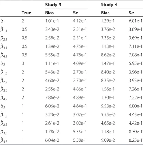
fork= 1, 2, 3. Table 1 presents the results for Studies 1 and 2 and Table 2 presents the results for Studies 3 and 4. We show the average biases (Bias) and standard errors (Se) for the estimates in both tables. Table 3 provides the passing rate of the proportional odds assumption (POA)

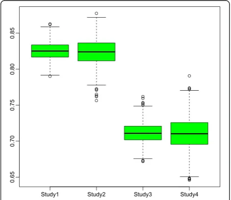
test, the HL test and both (POA&HL) tests for Studies 1 and 2. Table 3 depicts the results of the EHL test in Studies 3 and 4 among 1000 runs. Figure 1 shows the box plots of AUC scores for the four studies.

Note that, as expected, all four studies show that the three grid methods and the corresponding centralized method produce identical results. Hence, each table or figure presents the common results for the three grid models and the corresponding centralized model.

Two examples

In addition to simulation studies, we used two split public datasets to test our core model-fitting algorithm. The pur-pose was to illustrate how our core grid-fitting algorithm

Table 1 Common ordinal logistic regression estimates for three grid models with various local site sample sizes and the corresponding centralized model in Study 1 and Study 2

Study 1 Study 2

True Bias Se Bias Se

^

α1 −1 −4.75e-3 1.27e-1 −1.46e-2 1.82e-1 ^

α2 0 −1.17e-3 1.23e-1 −3.47e-3 1.75e-1 ^

α3 1 1.93e-3 1.30e-1 1.02e-2 1.84e-1 ^

β1 1 7.22e-3 8.02e-2 5.53e-3 1.14e-1 ^

β2 1 6.60e-3 8.02e-2 3.79e-3 1.14e-1 ^

β3 1 1.04e-2 1.42e-1 1.64e-3 2.01e-1 ^

β4 1 7.34e-3 1.42e-1 1.36e-2 2.02e-1

Table 2 Common multinomial logistic regression estimates for three grid models and the corresponding centralized model in Study 3 and Study 4

Study 3 Study 4

True Bias Se Bias Se

^

α1 2 1.01e-1 4.12e-1 1.29e-1 6.01e-1 ^

β1;1 0.5 3.43e-2 2.51e-1 3.76e-2 3.69e-1 ^

β2;1 0.5 2.58e-2 2.51e-1 3.35e-2 3.69e-1 ^

β3;1 0.5 1.39e-2 4.75e-1 1.13e-1 7.11e-1 ^

β4;1 0.5 5.55e-2 4.78e-1 8.62e-2 7.08e-1 ^

α2 3 1.11e-1 4.09e-1 1.47e-1 5.95e-1 ^

β1;2 2 5.43e-2 2.70e-1 8.40e-2 3.96e-1 ^

β2;2 2 4.60e-2 2.70e-1 8.35e-2 3.95e-1 ^

β3;2 2 2.55e-2 4.86e-1 1.56e-1 7.26e-1 ^

β4;2 2 7.86e-2 4.89e-1 1.30e-1 7.22e-1 ^

α3 1 6.06e-2 4.64e-1 5.53e-2 6.80e-1 ^

β1;3 1 3.23e-2 3.02e-1 5.55e-2 4.43e-1 ^

β2;3 1 2.61e-2 3.02e-1 4.65e-2 4.42e-1 ^

β3;3 1 1.78e-2 5.55e-1 1.18e-1 8.30e-1 ^

(6)

works. Note that these are not real multi-center studies but used for illustration purposes.

The first example is about the low birth weight data-set, which was obtained from Hosmer and Lemeshow [9] and contains 189 observations with 9 non-redundant variables. We picked 8 variables including AGE, RACE, SMOKE, PTL, HT, UI, FTV, BWTfrom the dataset, and reasonably modified several variables to create a new dataset as follows.RACEis a three-category variable, re-placed by two binary variables: OTHERvsWHITE and BLACKvsWHITE, respectively. PTL is the number of premature labors with values of 0, 1, etc., and was di-chotomized into 0 and greater than 0.FTVis the num-ber of physician visits, which is also dichotomized into 0 and greater than 0 as well. BWT is the birth weight in grams and it was categorized into 4 values (1, 2, 3 ,4) using cutoffs 3500, 3000 and 2500. AGE, SMOKE, HT, UI were kept as original, where AGE is continuous, SMOKE is binary, HT is binary variable for “History of hypertension", andUIis binary variable for“Presence of uterine irritability". We denote the new dataset as LBW.

To test the grid model fitting, we randomly picked 95 observations from LBW to create dataset LBW1 and the rest 94 observations to create LBW2.BWT is chosen as the 4-category response variable and the rest are covari-ates. Since the response is ordinal, we fitted a grid or-dinal logistic model without pooling LBW1 and LBW2. Suppose the fitted value forlog_{Pr BW T}Pr BW T_ðð _>≤k_kÞ_Þ(k= 1, 2, 3) is

^

αkþβ^1AGEþ^β2OTHERvsWHITE

þ^β3BLACKvsWHITEþ^β4SMOKEþβ^5PTL

þ^β6HTþβ^7UIþβ^8FTV:

Table 4 shows the model coefficient estimates (Est) and their standard errors (Se), with z-values (Zval) equal to the ratios of Est values over according Se values and p-values (Pval) to test whether Zval is significantly differ-ent than 0.

The grid proportional odds assumption test was also performed and resulted in a p-value of 0.366. Hence, there is no evidence to show that the assumption for the ordinal logistic model was invalid. To justify the grid model fitting, the ordinal logistic model was also fitted for LBW1 and for LBW2, separately. Grid AUC score (GAUC), AUC score for the model fitted by LBW1 (AUC1), and AUC score for the model fitted by LBW2 (AUC2) were all evaluated by 10-fold cross validation:

GAUC¼0:665;AUC1¼0:645;AUC2¼0:568:

Note that in this example the data are randomly split so every subset has the same underlying population. Hence, small AUC values only result from smaller sam-ple sizes (in subgroups). In addition, a grid HL test for grid model and HL tests for two separate models were performed using 10-fold cross validation with the same data partitions. Unfortunately, none of these models passed the HL test. This may be related to nonlinear effects of the

Table 3 Common passing rate of the model assumption test and the model fit test in each study for three grid models and the corresponding centralized model

POA* HL POA&HL

Study 1 0.967 0.579 0.559

Study 2 0.964 0.532 0.511

EHL

Study 3 0.554

Study 4 0.511

*POA: proportional odds assumption; EHL: extended HL test.

Figure 1Common box plots of AUC scores for four studies based on 1000 runs for three grid models and the corresponding centralized model.

Table 4 Grid ordinal logistic model fitting by separate low birth weight datasets

Est Se Zval Pval

^

α1 −0.415 0.719 −0.578 0.562 ^

α20 0.828 0.722 1.147 0.251 ^

α3 1.807 0.730 2.473 0.013

^

β1 0.016 0.027 0.594 0.552

^

β2 −0.980 0.339 −2.891 0.003 ^

β3 −1.245 0.424 −2.933 0.003 ^

β4 −1.028 0.318 −3.233 0.001 ^

β5 −0.915 0.419 −2.178 0.029 ^

β6 −0.991 0.618 −1.605 0.108 ^

β7 −0.972 0.402 −2.416 0.015 ^

(7)

continuous variable age, or to omitted interaction terms. However, as shown in simulation studies, failing to pass the HL test does not necessary mean the goodness-of-fit of these models are very poor.

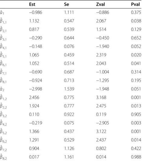
The second example is about Mammograph experi-ence data, which was also obtained from Hosmer and Lemeshow [9] and contains 412 observations with 6 var-iables. We kept the original dataset and only replaced multi-category variables by multiple binary variables. The generated new dataset was denoted as MAM and contained 9 variables:ME,SYMPT1,SYMPT2,SYMPT3, PB, HIST, BSE, DETC1 andDETC2. MEdenotes mam-mograph experience with “3 = never",“2 = within a year" and “1 = over a year ago". Original SYMPT was a 4-category variable and denoted the 4 responses to “you do not need a mammograph unless you develop symp-toms" from“strongly agree" to“strongly disagree". It was replaced by binary variables SYMPT1, SYMPT2 and SYMPT3. PB is a continuous variable for the degree of “perceived benefit of mammography". HIST is a binary variable for the response to whether “mother or sister has breast cancer history". BSEis the binary response to “Has anyone taught you how to examine your own breasts?". Original DECT was a 3-category variable and the response to “How likely is it that a mammogram could find a new case of breast cancer?". It was replaced by binary variablesDECT1 andDECT2.

We first randomly picked 206 observations from MAM to create datasetMAM1, and used the remaining 206 to createMAM2. We usedMEas the response. The multinomial logistic model was used to fit the dataset. We fitted a grid multinomial model without pooling MAM1and MAM2. Fork= 1, 2, suppose the fitted value forlogPr ME_{Pr ME}ð_ð ¼_¼k₃_ÞÞis

^

αkþβ^_1;kSYMPT1þβ^2;kSYMPT2þ^β3;kSYMPT3

þ^β_4;kPBþβ^5;kHISTþβ^6;kBSEþβ^7;kDETC1

þ^β8;kDECT2

Table 5 shows the model coefficient estimates (Est) and their standard errors (Se), with z-values (Zval) and p-values (Pval).

To justify the grid model fitting, a multinomial logistic model was also fitted forMAM1and forMAM2, separ-ately. However, both separate models produced invalid estimates (with very large standard errors). The invalid estimates are probably due to the small number of sub-jects with ME= 2 after splitting the dataset, and the large number of parameters. This obviously shows the need for grid model fitting based on datasets MAM1 and MAM2 when they are not allowed to be pooled. Ten-fold cross validation was used to evaluate extended AUC score and we performed the extended HL test for

the grid fitted model. The grid AUC score was 0.626 and the grid fitted model passed the extended HL test.

Discussion

While our focus was on multi-category logit models, the grid MLE method is applicable for grid computing for various likelihood type estimation problems including other generalized linear models and generalized estimat-ing equation models. However, when the likelihood is not separable for observations, then grid MLE may not work. For example, the Cox proportional hazards regres-sion adopts a profile likelihood that cannot be split by observations. Hence, more effort is necessary to design a grid model for Cox proportional odds regression, which was discussed in our recent publication [19].

For the proposed grid HL test and grid AUC,Yvalues are pooled directly and not protected. To protectY, the patient outcome values, we could adopt the methods proposed by Wu et al. [6] for the Grid HL test and the AUC score calculation, which avoid exchangingYvalues. These methods are accomplished through using trans-mitted locally predicted probabilities and their orders. Details are given in Algorithms 1 and 2 in Wu et al. [6].

In practice, the grid model fitting using multi-site data is more complicated than what is described in this manu-script (we focused on the model fitting step). Very often, it is necessary to conduct data pre-processing before the model fitting. For example, gender may use a coding method in different sites. Hence, data harmonization is

Table 5 Grid multinomial logistic model fitting by separate mammography datasets

Est Se Zval Pval

^

α1 −0.986 1.111 −0.886 0.375 ^

β1;1 1.132 0.547 2.067 0.038 ^

β2;1 0.817 0.539 1.514 0.129 ^

β3;1 −0.290 0.644 −0.450 0.652 ^

β4;1 −0.148 0.076 −1.940 0.052 ^

β5;1 1.065 0.459 2.319 0.020 ^

β6;1 1.052 0.514 2.043 0.041 ^

β7;1 −0.690 0.687 −1.004 0.314 ^

β8;1 −0.924 0.713 −1.295 0.195 ^

α2 −2.998 1.539 −1.948 0.051 ^

β1;2 2.456 0.775 3.168 0.001 ^

β2;2 1.924 0.777 2.475 0.013 ^

β3;2 0.110 0.922 0.119 0.905 ^

β4;2 −0.219 0.075 −2.905 0.003 ^

β5;2 1.366 0.437 3.122 0.001 ^

β6;2 1.291 0.529 2.437 0.014 ^

β7;2 0.904 1.126 0.802 0.422 ^

(8)

necessary before the grid model can be fitted. Another issue is missing data. One way to mitigate the problem is to deal with missing data during the pre-processing step using the same grid protocol across all sites. Another ap-proach is to handle missing data in the grid model-fitting step, which would be cumbersome. Additionally, some-times there are too many variables to fit the model; vari-able selection may thus be needed. Varivari-able selection usually requires the construction of models and it can be incorporated into the model-fitting step. Different sites may have different variables, so choosing and harmonizing the values of common variables needs to be done before the model-fitting step. For the proposed grid models, we assumed that the data were uniformly distributed across local clinical sites, and treated the data from each local site as a random sample from the whole dataset. However, this assumption may not hold and we will consider cluster ef-fects from different sites in our future work. We described (on page 4) that steps 1 and 2 for the grid model-fitting step need to be repeated until convergence. Each site needs to send the first derivative and Hessian matrices multiple times, which means that a reliable data transmis-sion function is necessary for successfully fitting a grid model. Recently we produced a reliable webservice called WebGLORE for binary logistic grid fitting [20]. In our set-ting the data transmission was adequate but there may be settings in which this may not be the case.

Conclusion

In the proposed grid methods, individual-level observa-tion data were never shared during the model fitting process. This offers a practical solution for mitigating privacy issues caused by pooling all data into a central site. Grid ordinal and multinomial logistic models were introduced in detail. In terms of increasing sample sizes, grid computing is more valuable for multi-category re-sponse logistic model than it is for binary logistic regres-sion, since the larger number of coefficient estimates in multi-category models obviously require more observa-tions. A small sample size might result in estimations with very large bias or standard error. The ordinal logis-tic model was proposed to only address the ordinal re-sponse data. The multinomial logistic model is used to deal with nominal response data, which requires even more coefficients and hence more observations for proper estimation when compared to the ordinal logistic model. The theory guarantees that the proposed grid Newton method achieves accurate estimation, which is the same as the one of the classical centralized Newton method. This is consistent with simulation study results. As shown in the simulation studies, the HL test and its extension might be too strong for assessing model fit and might produce false significant test results. These are limitations for the HL test, which are discussed by

Vittinghoff et al. [21]. Hence, other model fit assess-ment methods introduced by Hosmer and Lemeshow [9] could be used in addition to the extended HL test for the multinomial logistic model, and other methods for binary logistic model fit assessment could be used in addition to the HL test for the ordinal logistic model.

Additional file

Additional file 1:Gradients and Hessian matrices.In this file we provide the gradients and the Hessian matrices for all log-likelihood functions used in this manuscript.

Competing interests

The authors declare that they have no competing interests.

Authors_’contributions

YW drafted the majority of the manuscript and developed the models. XJ and SW provided detailed edits and discussion about the proposed model. WJ and PL helped on the implementation. LOM guided the experimental design and provided detailed edits to the manuscript. All authors read and approved the final manuscript.

Acknowledgements

We owe thanks to the Editor and two reviewers for their helpful and constructive comments and suggestions that helped improve the manuscript from earlier versions.

Publication of this article has been funded in part by NIH grants U54HL108460, K99HG008175, R00LM011392, R21LM012060, and PCORI contract CDRN-1306-04819.

Author details

1

Department of Biostatistics & Bioinformatics, Duke University, Durham, NC 27708, USA.2_{Division of Biomedical Informatics, Department of Medicine,} University of California, San Diego, La Jolla, CA 92093, USA.3Department of Electronic Engineering, Shanghai Jiaotong University, Shanghai 200240, China.

Received: 18 January 2014 Accepted: 15 January 2015

References

1. Ohno-Machado L, Agha Z, Bell DS, Dahm L, Day ME, Doctor JN, et al. pSCANNER team: patient-centered Scalable National Network for Effectiveness Research. J Am Med Informatics Assoc. 2014; 21:amiajnl–2014. doi:10.1136/amiajnl-2014-002751

2. Crandall W, Kappelman MD, Colletti RB, Leibowitz I, Grunow JE, Ali S, et al. ImproveCareNow: The development of a pediatric inflammatory bowel disease improvement network. Inflamm Bowel Dis. 2011;17:450–7. doi:10.1002/ibd.21394.

3. Kamath PS, Kim W. The model for end-stage liver disease (MELD). Hepatology. 2007;45:797–805.

4. Kennedy RL, Burton AM, Fraser HS, McStay LN, Harrison RF. Early diagnosis of acute myocardial infarction using clinical and electrocardiographic data at presentation: derivation and evaluation of logistic regression models. Eur Hear J. 1996;17:1181–91.

5. Boxwala AA, Kim J, Grillo JM, Ohno-Machado L. Using statistical and machine learning to help institutions detect suspicious access to electronic health records. J Am Med Inf Assoc. 2011;18:498–505.

6. Wu Y, Jiang X, Kim J, Ohno-Machado L. Grid Binary LOgistic REgression (GLORE): building shared models without sharing data. J Am Med Inform Assoc. 2012;2012:758–64. doi:10.1136/amiajnl-2012-000862.

7. Wang S, Jiang X, Wu Y, Cui L, Cheng S, Ohno-Machado L. EXpectation Propagation LOgistic REgRession ( EXPLORER ): Distributed Privacy-Preserving Online Model Learning. J Biomed Inform. 2013;46:480–96.

(9)

9. Hosmer DW, Lemeshow S. Applied logistic regression. New York: Wiley-Interscience 2000. http://books.google.com/books?hl=en&lr=&id=Po0RLQ7USIM- C&oi=fnd&pg=PA1&dq=Applied+logistic+regression&ots=D-n7Usc1kAR&sig=vR7mj7OsZ8DMsnvS19BsT30Ad8c (accessed 15 Mar2012). 10. Bradley AP. The use of the area under the ROC curve in the evaluation of

machine learning algorithms. Pattern Recognit. 1997;30:1145–59. 11. Hand DJ, Till RJ. A simple generalisation of the area under the ROC curve

for multiple class classification problems. Mach Learn. 2001;45:171–86. 12. Van Calster B, Van Belle V, Vergouwe Y, Steyerberg EW. Discrimination ability

of prediction models for ordinal outcomes: Relationships between existing measures and a new measure. Biometrical J. 2012;54:674–85.

13. Yang H, Carlin D. ROC surface: a generalization of ROC curve analysis. J Biopharm Stat. 2000;10:183–96.

14. Dreiseitl S, Ohno-Machado L, Binder M. Comparing three-class diagnostic tests by three-way ROC analysis. Med Decis Mak. 2000;20:323–31. 15. Brant R. Assessing Proportionality in the Proportional Odds Model for

Ordinal Logistic Regression. Biometrics. 1990;46:1171–8.

16. Williams R. Generalized ordered logit/partial proportional odds models for ordinal dependent variables. Stata J. 2006;6:58–82.

17. Fagerland MW, Hosmer DW. A goodness-of-fit test for the proportional odds regression model. Stat Med. 2013;32:2235–49.

18. Fagerland MW, Hosmer DW, Bofin AM. Multinomial goodness-of-fit tests for logistic regression models. Stat Med. 2008;27:4238–53.

19. Lyles RH. Regression Methods in Biostatistics: Linear, Logistic, Survival, and Repeated Measures Models. J Am Stat Assoc. 2006;101:403–4.

20. Lu C, Wang S, Ji Z, Wu Y, Xiong L, Jiang X, et al. WebDISCO: a Web service for DIStributed COx model learning without patient-level data sharing. In: Translational Bioinformatics Conference (accepted). 2014.

21. Jiang W, Li P, Wang S, Wu Y, Xue M, Ohno-Machado L, et al. WebGLORE: a web service for Grid LOgistic REgression. Bioinformatics. 2013;29:3238–40. doi: 10.1093/bioinformatics/btt559.

Submit your next manuscript to BioMed Central and take full advantage of:

• Convenient online submission

• Thorough peer review

• No space constraints or color ﬁgure charges

• Immediate publication on acceptance

• Inclusion in PubMed, CAS, Scopus and Google Scholar

• Research which is freely available for redistribution