S O F T W A R E
Open Access
ROCKETSHIP: a flexible and modular
software tool for the planning, processing
and analysis of dynamic MRI studies
Samuel R. Barnes
1†, Thomas S. C. Ng
1,2*†, Naomi Santa-Maria
1, Axel Montagne
3, Berislav V. Zlokovic
3and Russell E. Jacobs
1Abstract
Background:Dynamic contrast-enhanced magnetic resonance imaging (DCE-MRI) is a promising technique to characterize pathology and evaluate treatment response. However, analysis of DCE-MRI data is complex and benefits from concurrent analysis of multiple kinetic models and parameters. Few software tools are currently available that specifically focuses on DCE-MRI analysis with multiple kinetic models. Here, we developed ROCKETSHIP, an open-source, flexible and modular software for DCE-MRI analysis. ROCKETSHIP incorporates analyses with multiple kinetic models, including data-driven nested model analysis.
Results:ROCKETSHIP was implemented using the MATLAB programming language. Robustness of the software to provide reliable fits using multiple kinetic models is demonstrated using simulated data. Simulations also demonstrate the utility of the data-driven nested model analysis. Applicability of ROCKETSHIP for both preclinical and clinical studies is shown using DCE-MRI studies of the human brain and a murine tumor model.
Conclusion:A DCE-MRI software suite was implemented and tested using simulations. Its applicability to both preclinical and clinical datasets is shown. ROCKETSHIP was designed to be easily accessible for the beginner, but flexible enough for changes or additions to be made by the advanced user as well. The availability of a flexible analysis tool will aid future studies using DCE-MRI.
A public release of ROCKETSHIP is available at https://github.com/petmri/ROCKETSHIP.
Keywords:DCE-MRI, Imaging, ADC, Parametric mapping, Data-driven kinetic modelling, MATLAB, MRI, Nested model
Background
The utility of dynamic magnetic resonance imaging (MRI) studies to diagnose diseases, characterize their progression, and evaluate treatment response is a topic of vigorous research. In particular, physiological informa-tion garnered from techniques such as diffusion MRI, blood oxygen-level dependent (BOLD) MRI, iron-oxide imaging, dynamic susceptibility MRI (DSC-MRI) and dynamic contrast-enhanced MRI (DCE-MRI) [1] are being
explored as imaging biomarkers in virtually all aspects of medicine, especially in oncology and neurological diseases. DCE-MRI involves the rapid serial acquisition of T1-weighted images before, during and after intravenous injection of a contrast agent (CA). The physiological prop-erties of the tissue of interest are inferred by analyzing the image signal change kinetics induced by the CA within the tissue region of interest (ROI). Given the inherent leakiness of tumor blood vessels (which enhances the sig-nal observed at the tumor site due to more CA leakage) [2], the majority of DCE-MRI studies have focused on oncology applications [3]. Studies have especially focused on using DCE-MRI to characterize tumor phenotypes or to evaluate the response of tumors to therapy [4]. The use of DCE-MRI has also been explored in other fields such as obstetrics [5] and the neurosciences [6, 7].
* Correspondence:[email protected] †Equal contributors
1
Division of Biology and Biological Engineering, California Institute of Technology, Pasadena, CA 91125, USA
2
Department of Medicine, University of California, Irvine Medical Center, Orange, CA, USA
Full list of author information is available at the end of the article
Although several individual studies have demonstrated the promise of DCE-MRI as an imaging biomarker, wide-spread clinical adoption of this technique remains limited. This is in part because implementation and standardization of DCE-MRI is challenging. Differences in hardware such as the MRI field strength, coil setups and sequence types available at different institutions can affect the quality of the images acquired and constrain the choice of certain parameters such as the volume of interest, spatial and temporal resolution. The choice of contrast agent, each with unique pharmacokinetic properties and thus behavior in vivo [8], also vary greatly between studies. These factors can significantly affect the quality of the parametric maps generated from imaging data [9].
Widespread variability also exists in the processing and analysis of DCE-MRI data. Both semi-quantitative [10, 11] and quantitative parameters [12] are used to analyze the acquired signal intensity time curves. Several studies have demonstrated the utility of either type of parameters to characterize tumor tissues or monitor treatment response [13, 14]. However, challenges remain in determining the specificity of different parameters to the underlying physi-ology, development of robust quantification techniques for quantitative model fitting (such as the assignment of a robust arterial input function [15] or T1 measurement of tissues [16]), and the selection of appropriate equations or models to fit the acquired data [17].
Recent studies have sought to address and understand these issues. For example, both Cramer et al. [18] and Montagne et al. [6] demonstrated that the Patlak method may accurately estimate the vascular permeability in the intact or near intact blood brain barrier (BBB); a chal-lenge given the low permeability values being consid-ered (Ktrans< 0.3 mL/100 g/min) [19–21]. In particular, Montagne et al. were able to demonstrate significant differences in permeability within grey and white matter between human subjects with no cognitive impairment, mild cognitive impairment, and with age [6] using Patlak analysis. Two-compartment models have been shown to be more appropriate at higher permeability [18, 22]. Ewing et al. have explored the use of nested model-selection to determine the appropriate physiological models to fit both preclinical and clinical DCE-MRI data [23, 24], while Jackson et al. recently showed good correlation of semi-quantitative metrics with parameters derived from an extended Tofts model in patients with Type 2 Neuro-fibromatosis [13]. Importantly, these studies suggest that robust analysis of DCE-MRI data may be disease and organism specific and that a data-driven approach that con-siders a library of processing and analytical methods may be necessary and appropriate for DCE-MRI analysis [12].
Exploration of these different types of DCE-MRI pro-cessing and analyses would be facilitated with standard-ized software. Software standardization can reduce biases
and errors that may arise from the type of processing algo-rithm used for fitting and enable more consistent compar-isons between studies. Moreover, availability of a flexible, easily modifiable and extensible software suite allows the researcher/clinician to examine how various factors dis-cussed above may apply to their specific DCE-MRI study.
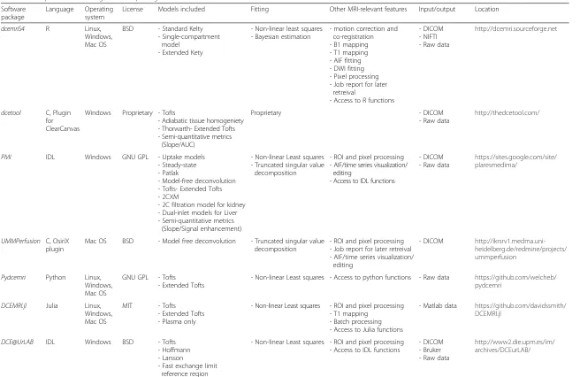
To date, numerous software packages are available for DCE-MRI analysis. These include general purpose phar-macokinetic analysis packages such as PMOD (pmod.com), WinSAAM [25], JPKD (pkpd.kmu.edu.tw/jpkd) or SAAMII [26]. These packages are often complex to use, are only commercially available and/or require significant pre-processing of the data to adjust for DCE-MRI usage. DCE-MRI specific software packages also exist, includ-ing commercially available packages licensed for clinical use [27]. While these are often user friendly and directly integrated with PACS databases, details about each pack-age’s implementation and certain options involved in the fitting algorithms may be unavailable. This can lead to a wide variability in output results [27]. Other packages available include PMI (https://sites.google.com/site/plares-medima/), pydcemri (github.com/davidssmith/pydcemri), DCEMRI.jl [28], Jim (Xinapse Systems Ltd), BioMap (maldi-msi.org), PermGUI/PCT [29], Toppcat [30], DCEM-RIS4 [31], dcetool (http://thedcetool.com/), dcemri (http:// dcemri.sourceforge.net/), DATforDCEMRI [32], DCE@ UrLAB [33] and UMMPerfusion [34]. Table 1 provides a summary of the capabilities of these packages. While geared for DCE-MRI, most of them are limited in the range of fit-ting methods, models and parameters that can be analyzed. A number of the packages (developed using IDL and C) are built around a graphical user interface (GUI) that needs to be recompiled each time a new functionality is implemented or a setting changed, which can make mod-ule development and individualized changes non-trivial for a novice user. None of the currently available packages in Table 1 enable recently developed data-driven methods, such as nested-model selection, that analyze the appropri-ateness of the models and parameters being used and generated [23, 24, 35–37]. To circumvent these con-straints, groups often develop in-house software for their studies [38–41], with limited availability for other users. This hinders adoption of these methods for widespread use and testing.
dcemriS4 R Linux, Windows, Mac OS
BSD - Standard Kelty - Single-compartment
model - Extended Kety
- Non-linear least squares - Bayesian estimation
- motion correction and co-registration - B1 mapping - T1 mapping - AIF fitting - DWI fitting - Pixel processing - Job report for later
retreival
- Access to R functions
- DICOM - NIFTI - Raw data
http://dcemri.sourceforge.net
dcetool C, Plugin for ClearCanvas
Windows Proprietary - Tofts
- Adiabatic tissue homogeniety - Thorwarth- Extended Tofts - Semi-quantitative metrics
(Slope/AUC)
Proprietary - DICOM
- Raw data
http://thedcetool.com/
PMI IDL Windows GNU GPL - Uptake models - Steady-state - Patlak
- Model-free deconvolution - Tofts- Extended Tofts - 2CXM
- 2C filtration model for kidney - Dual-inlet models for Liver - Semi-quantitative metrics
(Slope/Signal enhancement)
- Non-linear Least squares - Truncated singular value
decomposition
- ROI and pixel processing - AIF/time series visualization/
editing
- Access to IDL functions
- DICOM - Raw data
https://sites.google.com/site/ plaresmedima/
UMMPerfusion C, OsiriX plugin
Mac OS BSD - Model free deconvolution - Truncated singular value decomposition
- ROI and pixel processing - Job report for later retreival - AIF/time series visualization/
editing
- DICOM http://ikrsrv1.medma.uni-heidelberg.de/redmine/projects/ ummperfusion
Pydcemri Python Linux, Windows, Mac OS
GNU GPL - Tofts - Extended Tofts
- Non-linear Least squares - Access to python functions - Raw data https://github.com/welcheb/ pydcemri
DCEMRI.jl Julia Linux, Windows, Mac OS
MIT - Tofts - Extended Tofts - Plasma only
- Non-linear Least squares - ROI and pixel processing - T1 mapping
- Batch processing - Access to Julia functions
- Matlab data https://github.com/davidssmith/ DCEMRI.jl
DCE@UrLAB IDL Windows BSD - Tofts - Hoffmann - Larsson
- Fast exchange limit reference region
- Non-linear Least squares - ROI and pixel processing - Access to IDL functions
- DICOM - Bruker - Raw data
http://www2.die.upm.es/im/ archives/DCEurLAB/
BMC
Medical
Imaging
(2015) 15:19
Page
3
of
(AUC, MRT
- mean residence time)
TOPPCAT Javascript, ImageJ plugin
Linux, Windows, Mac OS
BSD - Patlak - Non-linear
Least squares
- T1 mapping - Access to ImageJ
functions
- ImageJ readable data formats
https://dblab.duhs.duke.edu/ modules/dblabs_topcat/
Jim Java Linux,
Windows, Mac OS
Proprietary - Tofts - Extended Tofts - One
compartment - Fermi - 2CXM
- Semi-quantitative metrics (AUC)
Proprietary - ROI and pixel processing
- DICOM - Analyze - Bruker - Commercial
formats - Raw data
http://www.xinapse.com/ Manual/index.html
PermGUI Matlab Windows Creative Commons
- Patlak - T1 mapping
- ROI and pixel processing
- DICOM - Analyze - NIFTI
http://www.quantilyze.com/ permgui/
BioMap IDL Linux, Windows, Mac OS
Proprietary - Extended Tofts - Non-linear Least squares
- T1 fitting - DICOM
- Analyze - TIF/PNG
http://www.maldi-msi.org/
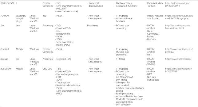
ROCKETSHIP Matlab Linux, Windows, Mac OS
GNU GPL - Tofts - Extended Tofts - Fast exchange regime
(FXR) - 2CXM - Tissue uptake - Nested-model selection - Patlak
- Semi-quantitative metrics (AUC)
- Non-linear Least squares
- T1 mapping - ROI and pixel
processing - AIF fitting/import - DWI fitting - Job report for
later retreival
- AIF/time series visualization/ editing
- Batch processing - Access to Matlab functions - Model fit comparisons with
statistical metrics - Drift correction
- DICOM - Analyze - NIFTI - Raw data - Matlab data
https://github.com/petmri/ ROCKETSHIP
*Excludes commerical packages for clinical use, AUC: area under curve, DWI: diffusion-weighted imaging
BMC
Medical
Imaging
(2015) 15:19
Page
4
of
and analyses with a library of common pharmacokinetic modeling methods as well as recently developed statisti-cally driven nested model methods. Implementation of ROCKETSHIP in a commonly used language (MATLAB) for image analysis should allow both novice and advance users to utilize and extend the software for their specific DCE-MRI applications.
We test the robustness of this software tool using sim-ulations and demonstrate the utility of ROCKETSHIP to analyze preclinical and clinical DCE-MRI data from different disease models.
Implementation
All components of ROCKETSHIP were implemented in the MATLAB environment, specifically MATLAB release 2014a. Detailed description of each component can be found in source code comments and documentation that is accessible at the project’s github page (https://github.-com/petmri/ROCKETSHIP). In this section, we describe the general architecture of the software suite, and high-light the key aspects of the software and the algorithms currently implemented in the software.
Architecture design and GUI description
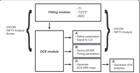
A simplified schematic outlining the design of ROCKET-SHIP is shown in Fig. 1. The software is divided into discrete modules to separate processing and analysis components of the pipeline. Initially, a fitting module GUI is available for the user to generate voxel-wide parametric maps directly from imaging data. Common MRI parameters such as T2 (and T2*) and T1 relaxation times, and apparent diffusion coefficients (ADC) from diffusion MRI data can be estimated with different fit-ting methods. A summary of the equations used is in Appendix A. Additional user specified fitting functions can be easily implemented without major modifications to the GUI.
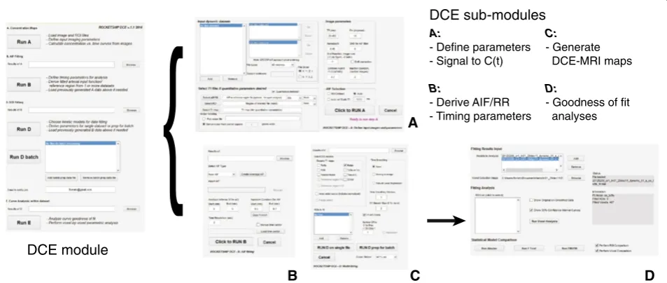
ROCKETSHIP is particularly focused on the process-ing and analysis of MRI data. Within the DCE-MRI module (Fig. 2), sub-modules are implemented that focus on:
1) Preparation of the dynamic datasets for DCE-MRI analysis. This involves options for intensity data to concentration versus time curves conversion using T1 maps, selection of the AIF or reference region (RR) and the ROI, noise filtering and signal intensity drift correction over the dynamic time course (Fig.2a). A summary of how these are implemented is provided inAppendix B.
2) AIF or RR processing with temporal truncation. This sub-module allows the appropriate AIF/RR to be selected. The raw or fitted AIF (currently limited to bi-exponential fitting) from an individual dataset can be used (Fig.2b). Alternatively, multiple AIFs/RRs can be combined to form a population-averaged AIF/RR. A summary of the implementation is provided in
Appendix C. As time duration and temporal resolution can be critical for analysis, options to modify these factors are included.
3) Derivation of DCE-MRI parametric maps (Fig.2c). Multiple pharmacokinetic models and semi-quantitative metrics can be fitted using ROCKETSHIP. In the current implementation, the Tofts, extended Tofts, Patlak, shutter-speed, two-compartment exchange, tissue uptake models and the area-under-curve (AUC) metric can be calculated (Table1). Details about these models are summarized inAppendix D. Apart from these stand-alone models, a nested model method is also implemented.
Nesting is based on the hierarchy inherent within the two-compartment exchange model; the algorithm was developed, tested and described in detail by Ewing et al. [12, 23, 24, 37]. First, DCE-MRI data are fitted to the zero-order model, which describes the case where there is insufficient evidence of filling of the vasculature with CA [23, 37]. Next, the initial fit is compared to the data fitting using the one parameter steady-state model:
C tð Þ ¼v Cað Þt ð1Þ WhereC(t) is the concentration of the CA in the voxel of interest at time t, v is the volume fraction of the indica-tor distribution space and Ca(t) is the concentration of the CA in the arterial compartment at time t. Here, v can represent the plasma volume fraction (vp) in a voxel that is highly vascularized with no vascular/extravascular ex-change, the extravascular volume fraction (ve) in a weakly vascularized voxel, or v = vp+ ve in a fast-exchange sce-nario. A statistical F-test is used to evaluate the likelihood
that an observed improvement of fit to the data, using a model with higher number of parameters, warrants the use of additional parameters [42]. A p-value <0.05 is used as a criterion to increase the number of parame-ters in the model fit.
In the current implementation, the Patlak model repre-sents the two-parameter form of the two-compartment model with the extended Tofts model with three parame-ters being at the top of the nested hierarchy [23, 24, 37].
Options to smooth the dynamic signal time course and to fit specific ROIs versus voxel-by-voxel fitting are also available in the DCE-MRI sub-module (Fig. 2c).
4) While models belonging to the same hierarchy can be folded into the nested model fitting option, it may be desirable to compare non-nested models or make comparisons with different statistical tests. The fitting analysis sub-module allows for visual and statistical assessment of goodness-of-fit (Fig. 2d). Model fits with 95 % prediction bounds of the fit are shown graphically along with the raw data for each voxel/ROI. Fits between models can be compared using the F-test [42, 43], fraction of modeled information (FMI) and fraction of residual information (FRI) [35], and the Akaike information criterion [7, 43]. These results can be exported to an Excel (office.microsoft.com/en-us/excel) spreadsheet for offline analysis.
Estimation of model parameters
All curve fitting functions in ROCKETSHIP are imple-mented using MATLAB’s Curve Fitting Toolbox. T1, T2 and ADC signal equations can be linearized and fitted with linear regression (See Appendix A). Alternatively, these parameters can be directly fitted with non-linear methods. ROCKETSHIP uses the trust region algorithm provided in the Curve Fitting Toolbox to perform non-linear least squares regression. For T1, T2 and ADC regres-sion, the parameters are hard-coded to have non-negative value constraints. Robust curve fitting is dependent on ap-propriate starting parameters for the fitting routine [44]. To facilitate this process, a preferences text file defining parameter constraints and convergence criteria, such as fitting tolerances and maximum numerical of iterations, is provided to allow easy editing of these variables. This text file is read by ROCKETSHIP when AIF and model fitting sub-modules are run.
During testing of ROCKETSHIP, it was found that Ktrans fitting often converged to local minima instead of the desired global minimum solution. To address this, Ktrans was fitted using multiple starting values with the fit value converging with the lowest residual used as the final value. Other variables were less sensitive to the starting position and thus a single initial value was used to fit each of those variables.
Voxel-wide fitting is performed in parallel using func-tions provided by MATLAB’s Parallel Computing Toolbox for increased performance.
{
DCE moduleA
B C D
A:
- Define parameters - Signal to C(t)
B:
- Derive AIF/RR - Timing parameters
C: - Generate DCE-MRI maps
D:
- Goodness of fit analyses DCE sub-modules
Inputs and outputs
To enable processing of both preclinical and clinical data, the software can read and write both NIFTI/Analyze and DICOM formats. ROIs can be input to ROCKETSHIP as image files drawn in other image visualization programs such as MRIcro (www.mricro.com) or as. roifiles gener-ated from ImageJ (imagej.nih.gov/ij).
Datasets can be processed through the pipeline individually. A batch mode is also available to generate multiple paramet-ric maps in thefittingand DCE-MRI model fitting modules.
Text files logging outputs from each module are stored and emailed to the user upon task completion. Data from each module in the processing pipeline are also stored in files to facilitate debugging, transfer between users and allows processing pauses between modules.
Results
Validation of ROCKETSHIP software with simulation
Precision and accuracy of individual kinetic model fitting The robustness of ROCKETSHIP was evaluated with simulations. Simulated datasets containing two (Tofts, Patlak models), three (Extended Tofts) and four parame-ters (two-compartment exchange model, 2CXM) were generated using MATLAB. The ability of ROCKETSHIP to recover the appropriate DCE-MRI parameter values from simulated data at different SNR and time resolutions was evaluated. To achieve this, curves were generated using specific parameter values defined in Table 2. For each parameter permutation Rician noise at different SNRs was added to the signal intensity versus time curves and fitted. This process was repeated with new noise 100 times in a Monte-Carlo manner to estimate the accuracy and precision of the fits. Resultant curves were fitted with ROCKETSHIP using the same model that was used to generate the curves. The population AIF published by
Parker et al. was used in all simulations [15]. Default fitting options were used. The accuracy of the fitted parameters were evaluated with the concordance correl-ation coefficient (CCC) [45].
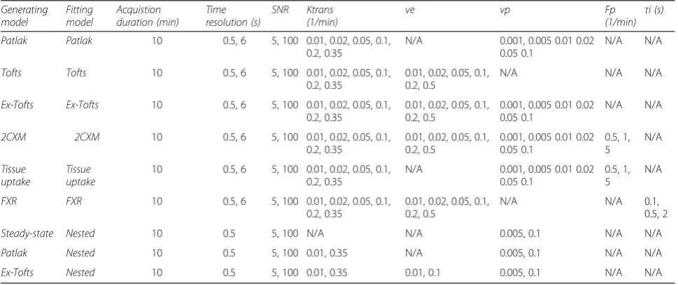
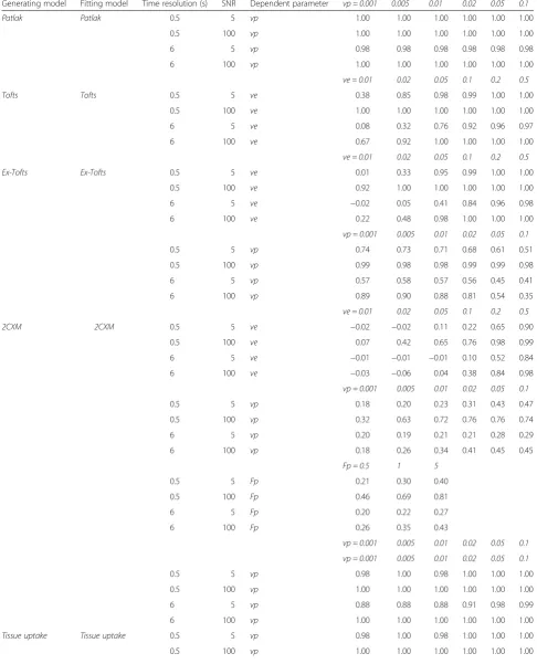
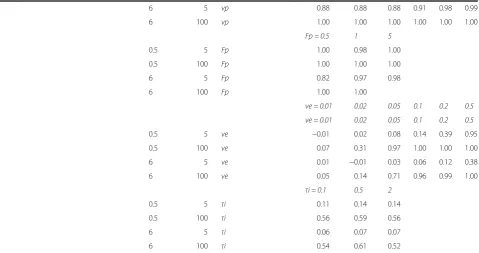
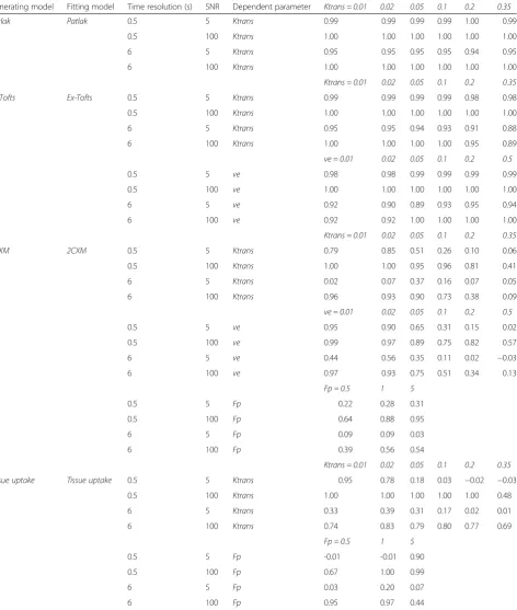
Figure 3 shows plots comparing fitted Ktransvalues to the values used to generate the simulated curves for different models. At high SNR and short time resolution, there is good concordance between simulated and fitted values. This is reflected in the CCC comparisons (Tables 3, 4 and 5). Fitting using ROCKETSHIP was generally able to recover parameter values with high accuracy and precision, as demonstrated by the small error bars seen in Fig. 3 and the high CCC values for the fitted to actual value comparisons across multiple models and with different parameters. Results shown in Fig. 3 and Tables 3, 4 and 5 demonstrate that ROCKETSHIP perform on par or better compared to QIBA simulation fittings using the Tofts model with DCE@UrLAB and DCEMRI.jl both qualitatively (com-pared to figures generated by DCE@UrLAB [33]) and quantitatively (CCC≥0.9 in general for Ktrans and ve recovery using Tofts model, similar to or better than the reported CCCs generated by DCEMRI.jl [28]). As with all curve fitting algorithms, the accuracy of the fit will be dependent on a number of factors [18], including SNR, sampling resolution and the number of parameters being fitted (Fig. 4, Tables 3, 4 and 5).
Accuracy of model selection using nested model analysis The data-driven, nested model analysis function in ROCK-ETSHIP was also tested. Simulation curves reflective of each level of nesting (steady-state, Patlak and extended Tofts models) were generated as above. The resultant curves were fitted using the nested method.
Simulation results using the nested model fitting are shown in Fig. 5 and Table 6. The nested model fitting was
Table 2Fitting parameters for simulation studies
Generating model
Fitting model
Acquistion duration (min)
Time resolution (s)
SNR Ktrans (1/min)
ve vp Fp
(1/min) τ i (s)
Patlak Patlak 10 0.5, 6 5, 100 0.01, 0.02, 0.05, 0.1,
0.2, 0.35
N/A 0.001, 0.005 0.01 0.02
0.05 0.1
N/A N/A
Tofts Tofts 10 0.5, 6 5, 100 0.01, 0.02, 0.05, 0.1,
0.2, 0.35
0.01, 0.02, 0.05, 0.1, 0.2, 0.5
N/A N/A N/A
Ex-Tofts Ex-Tofts 10 0.5, 6 5, 100 0.01, 0.02, 0.05, 0.1, 0.2, 0.35
0.01, 0.02, 0.05, 0.1, 0.2, 0.5
0.001, 0.005 0.01 0.02 0.05 0.1
N/A N/A
2CXM 2CXM 10 0.5, 6 5, 100 0.01, 0.02, 0.05, 0.1,
0.2, 0.35
0.01, 0.02, 0.05, 0.1, 0.2, 0.5
0.001, 0.005 0.01 0.02 0.05 0.1
0.5, 1, 5
N/A
Tissue uptake
Tissue uptake
10 0.5, 6 5, 100 0.01, 0.02, 0.05, 0.1, 0.2, 0.35
N/A 0.001, 0.005 0.01 0.02
0.05 0.1
0.5, 1, 5
N/A
FXR FXR 10 0.5, 6 5, 100 0.01, 0.02, 0.05, 0.1,
0.2, 0.35
0.01, 0.02, 0.05, 0.1, 0.2, 0.5
N/A N/A 0.1,
0.5, 2
Steady-state Nested 10 0.5 5, 100 N/A N/A 0.005, 0.1 N/A N/A
Patlak Nested 10 0.5 5, 100 0.01, 0.35 N/A 0.005, 0.1 N/A N/A
able to recover the appropriate model for the majority of the fitting curves. Accuracy of the nested model fitting was shown to be dependent on SNR. Lower SNR led to more model misclassification of voxels.
In vivo examples
Preclinical data set
DCE-MRI was performed on an athymic BLABL/c nude mouse bearing a HER2-expressing BT474 human breast cancer tumor. A 17β-estradiol pellet (Innovative Research of America) was implanted subcutaneously into the back of the mouse one day prior to orthotopic inoculation (6thand 9thmammary fat pad) of 5 × 10⁶cells in matrigel (BD Biosciences). The tumor volume was≈200 mm3at the time of imaging. Mouse care and experimental procedures were carried out in accordance with protocols approved by the Institutional Animal Care and Use Committee at Caltech.
Imaging was performed using a Biospec (Bruker-Biospin Inc. Billerica, MA) 7 T MRI scanner and a custom-built birdcage coil. The mouse was anesthetized during the ses-sion with 1.3-1.5 % isoflurane/air mixture. Body temperature was maintained at 36-37 °C with warmed air through the bore. A variable flip angle method was used to generate T1 maps. Gradient echo images (FLASH, FA = 12°, 24°, 36°, 48°, 60°, matrix size = 140 × 80, voxel size = 0.25 × 0.25 mm2, slice thickness = 1 mm, TR/TE = 200/2 ms) centered on the tumor (3 slices) and the left ventricle (1 slice) were acquired. Next, DCE-MRI was acquired (FLASH, FA = 35°, TR/ TE = 25/2 ms, geometry the same as the T1 maps, time resolution = 2 s, duration = 22 min). After a baseline of 2.5 min, Gd-DTPA (0.1 mmol/kg, Magnevist, Bayer) was injected intravenously via a tail vein catheter using a powered-injector (New Era Inc.) at 0.5 mL/min. Imaging
data were processed using ROCKETSHIP and analyzed with the nested model method.
Parametric maps and associated concentration vs. time curves are shown in Fig. 6. For this tumor, the extended Tofts model was deemed the most appropriate for the majority of the tumor. Generated Ktransvalues were similar to those observed in prior studies using the same tumor cell line [46]. Consistent with other studies, there is a heterogeneous distribution of Ktrans, veand vphighlighting a leaky and vascularized rim with a necrotic core.
Clinical data set
The clinical data set was obtained from a wider study set being accrued by the University of Southern California (USC) Alzheimer’s disease Research Center. The study was approved by the USC Institutional Review Board. The imaging dataset used here was obtained from one of the participants from the no cognitive impairment cohort, as determined from medical examination and neuropsycho-logical evaluation. All imaging was performed at the Keck Medical Center of USC. Participants underwent a medical examination, neuropsychological evaluations and blood draw to ensure appropriate kidney function for CA administration prior to imaging.
The imaging protocol performed was developed to study BBB changes in patients with cognitive impairment and is detailed in [6]. Briefly, all images were obtained on a GE 3 T HDXT MR scanner with a standard eight-channel array head coil. Anatomical coronal spin echo T2-weighted scans were first obtained through the hippocampi (TR/TE 1550/97.15 ms, NEX = 1, slice thickness 5 mm with no gap, FOV = 188 x 180 mm, matrix size = 384 x 384). Base-line coronal T1-weighted maps were then acquired using a T1-weighted 3D spoiled gradient echo (SPGR) pulse se-quence and variable flip angle method using flip angles of
A
B
C
Fig. 3Ktransfitting of simulated data. Simulated data with time resolution of 0.5 s and SNR = 100 were fitted using the same model used to generate the
simulation with ROCKETSHIP using default settings for the Patlak method (a), Tofts (b) and Extended Tofts models (c). Ktranssimulated vs. fitted
were plotted as a function of veand vp. Dashed line is unity. Error bars denote standard deviation. Given the similar fits, points for different veand vpmay
Table 3Concordance correlation coefficients (CCC) comparing fitted and simulated Ktrans using different models and dependent parameters
Generating model Fitting model Time resolution (s) SNR Dependent parameter vp = 0.001 0.005 0.01 0.02 0.05 0.1
Patlak Patlak 0.5 5 vp 1.00 1.00 1.00 1.00 1.00 1.00
0.5 100 vp 1.00 1.00 1.00 1.00 1.00 1.00
6 5 vp 0.98 0.98 0.98 0.98 0.98 0.98
6 100 vp 1.00 1.00 1.00 1.00 1.00 1.00
ve = 0.01 0.02 0.05 0.1 0.2 0.5
Tofts Tofts 0.5 5 ve 0.38 0.85 0.98 0.99 1.00 1.00
0.5 100 ve 1.00 1.00 1.00 1.00 1.00 1.00
6 5 ve 0.08 0.32 0.76 0.92 0.96 0.97
6 100 ve 0.67 0.92 1.00 1.00 1.00 1.00
ve = 0.01 0.02 0.05 0.1 0.2 0.5
Ex-Tofts Ex-Tofts 0.5 5 ve 0.01 0.33 0.95 0.99 1.00 1.00
0.5 100 ve 0.92 1.00 1.00 1.00 1.00 1.00
6 5 ve −0.02 0.05 0.41 0.84 0.96 0.98
6 100 ve 0.22 0.48 0.98 1.00 1.00 1.00
vp = 0.001 0.005 0.01 0.02 0.05 0.1
0.5 5 vp 0.74 0.73 0.71 0.68 0.61 0.51
0.5 100 vp 0.99 0.98 0.98 0.99 0.99 0.98
6 5 vp 0.57 0.58 0.57 0.56 0.45 0.41
6 100 vp 0.89 0.90 0.88 0.81 0.54 0.35
ve = 0.01 0.02 0.05 0.1 0.2 0.5
2CXM 2CXM 0.5 5 ve −0.02 −0.02 0.11 0.22 0.65 0.90
0.5 100 ve 0.07 0.42 0.65 0.76 0.98 0.99
6 5 ve −0.01 −0.01 −0.01 0.10 0.52 0.84
6 100 ve −0.03 −0.06 0.04 0.38 0.84 0.98
vp = 0.001 0.005 0.01 0.02 0.05 0.1
0.5 5 vp 0.18 0.20 0.23 0.31 0.43 0.47
0.5 100 vp 0.32 0.63 0.72 0.76 0.76 0.74
6 5 vp 0.20 0.19 0.21 0.21 0.28 0.29
6 100 vp 0.18 0.26 0.34 0.41 0.45 0.45
Fp = 0.5 1 5
0.5 5 Fp 0.21 0.30 0.40
0.5 100 Fp 0.46 0.69 0.81
6 5 Fp 0.20 0.22 0.27
6 100 Fp 0.26 0.35 0.43
vp = 0.001 0.005 0.01 0.02 0.05 0.1
vp = 0.001 0.005 0.01 0.02 0.05 0.1
0.5 5 vp 0.98 1.00 0.98 1.00 1.00 1.00
0.5 100 vp 1.00 1.00 1.00 1.00 1.00 1.00
6 5 vp 0.88 0.88 0.88 0.91 0.98 0.99
6 100 vp 1.00 1.00 1.00 1.00 1.00 1.00
Tissue uptake Tissue uptake 0.5 5 vp 0.98 1.00 0.98 1.00 1.00 1.00
2°, 5° and 10°. (TR/TE = 8.29/3.08 ms, NEX = 1, slice thick-ness 5 mm with no gap, FOV 188 x 180 mm, matrix size 160 x 160). Coronal DCE MRI covering the hippocampi and temporal lobes were acquired using a T1-weighted 3D SPGR pulse sequence (FA = 15°, TR/TE = 8.29/3.09 ms, NEX = 1, slice thickness 5 mm with no gap, FOV 188 x 180 mm, matrix size 160 x 160, voxel size was 0.625 x 0.625 x 5 mm3). This sequence was repeated for a total of 16 min with an approximate time resolution of 15.4 s. Gadobenate dimegulumine (MultiHance®, Braaco, Milan, Italy) (0.05 mmol/kg), a gadolinium-based CA, was admin-istered intravenously into the antecubital vein using a power injector, at a rate of 3 mL/s followed by a 25 mL saline flush, 30 s into the DCE scan. Imaging data were processed by ROCKETSHIP. The AIF, which was extracted from an ROI positioned at the internal carotid artery, was fitted with a bi-exponential function prior to fitting analysis with 2CXM.
Parametric maps and associated concentration vs. time curves are shown in Fig. 7. Compared to the murine tumor that contains leaky vasculature [41], Ktrans values for the human brain are lower, as expected given the intact blood brain barrier in normal human subjects [6]. As shown in Fig. 7e, the bi-exponential function estimated the AIF well and allowed for a good fit of concentration time curves within the brain parenchyma (Fig. 7f).
Discussion
Development and adoption of DCE-MRI by clinicians and researchers requires the availability of analysis software that not only has sufficient functionality for the novice end-user, but also the flexibility and extensibility capability for more complicated analyses. Using its default settings, users can follow ROCKETSHIP’s pipeline to generate para-metric maps of common kinetic models. Its modular design allows other models to be incorporated in a straightforward manner. Recently, several groups have recognized that data-driven approaches in selecting the appropriate model may be important for proper physiological interpretation of the DCE-MRI data [23]. To facilitate this, ROCKETSHIP includes a nested model fitting option as well as statistical tools to analyze and compare the goodness-of-fit between different kinetic models.
We selected the MATLAB environment for a number of reasons. Firstly, MATLAB is widely used for image analysis in the academic community; programs written in MATLAB can generally be run on Mac, Windows or Unix-based op-erating systems with minimal porting issues. Secondly, MATLAB provides several toolboxes (such as the Curve Fitting Toolbox and Parallel Computing Toolbox) that fa-cilitated development of the current software and allows fu-ture extensions to be easily implemented. MATLAB also has a strong user-contributed library of imaging processing
Table 3Concordance correlation coefficients (CCC) comparing fitted and simulated Ktrans using different models and dependent
parameters (Continued)
6 5 vp 0.88 0.88 0.88 0.91 0.98 0.99
6 100 vp 1.00 1.00 1.00 1.00 1.00 1.00
Fp = 0.5 1 5
0.5 5 Fp 1.00 0.98 1.00
0.5 100 Fp 1.00 1.00 1.00
6 5 Fp 0.82 0.97 0.98
6 100 Fp 1.00 1.00
ve = 0.01 0.02 0.05 0.1 0.2 0.5
ve = 0.01 0.02 0.05 0.1 0.2 0.5
0.5 5 ve −0.01 0.02 0.08 0.14 0.39 0.95
0.5 100 ve 0.07 0.31 0.97 1.00 1.00 1.00
6 5 ve 0.01 −0.01 0.03 0.06 0.12 0.38
6 100 ve 0.05 0.14 0.71 0.96 0.99 1.00
τi = 0.1 0.5 2
0.5 5 τi 0.11 0.14 0.14
0.5 100 τi 0.56 0.59 0.56
6 5 τi 0.06 0.07 0.07
6 100 τi 0.54 0.61 0.52
Table 4Concordance correlation coefficients (CCC) comparing fitted and simulated vp using different models and dependent parameters
Generating model Fitting model Time resolution (s) SNR Dependent parameter Ktrans = 0.01 0.02 0.05 0.1 0.2 0.35
Patlak Patlak 0.5 5 Ktrans 0.99 0.99 0.99 0.99 1.00 0.99
0.5 100 Ktrans 1.00 1.00 1.00 1.00 1.00 1.00
6 5 Ktrans 0.95 0.95 0.95 0.95 0.94 0.95
6 100 Ktrans 1.00 1.00 1.00 1.00 1.00 1.00
Ktrans = 0.01 0.02 0.05 0.1 0.2 0.35
Ex-Tofts Ex-Tofts 0.5 5 Ktrans 0.99 0.99 0.99 0.99 0.98 0.98
0.5 100 Ktrans 1.00 1.00 1.00 1.00 1.00 1.00
6 5 Ktrans 0.95 0.95 0.94 0.93 0.91 0.88
6 100 Ktrans 1.00 1.00 1.00 1.00 0.95 0.89
ve = 0.01 0.02 0.05 0.1 0.2 0.5
0.5 5 ve 0.98 0.98 0.99 0.99 0.99 0.99
0.5 100 ve 1.00 1.00 1.00 1.00 1.00 1.00
6 5 ve 0.92 0.90 0.89 0.93 0.95 0.94
6 100 ve 0.92 0.92 1.00 1.00 1.00 1.00
Ktrans = 0.01 0.02 0.05 0.1 0.2 0.35
2CXM 2CXM 0.5 5 Ktrans 0.79 0.85 0.51 0.26 0.10 0.06
0.5 100 Ktrans 1.00 1.00 0.95 0.96 0.81 0.41
6 5 Ktrans 0.02 0.07 0.37 0.16 0.07 0.05
6 100 Ktrans 0.96 0.93 0.90 0.73 0.38 0.09
ve = 0.01 0.02 0.05 0.1 0.2 0.5
0.5 5 ve 0.95 0.90 0.65 0.31 0.15 0.02
0.5 100 ve 0.99 0.97 0.89 0.75 0.82 0.57
6 5 ve 0.44 0.56 0.35 0.11 0.02 −0.03
6 100 ve 0.97 0.93 0.75 0.51 0.34 0.13
Fp = 0.5 1 5
0.5 5 Fp 0.22 0.28 0.31
0.5 100 Fp 0.64 0.88 0.95
6 5 Fp 0.09 0.09 0.03
6 100 Fp 0.39 0.56 0.54
Ktrans = 0.01 0.02 0.05 0.1 0.2 0.35
Tissue uptake Tissue uptake 0.5 5 Ktrans 0.95 0.78 0.18 0.03 −0.02 −0.03
0.5 100 Ktrans 1.00 1.00 1.00 1.00 1.00 0.48
6 5 Ktrans 0.33 0.39 0.31 0.17 0.02 0.01
6 100 Ktrans 0.74 0.83 0.79 0.80 0.77 0.69
Fp = 0.5 1 5
0.5 5 Fp -0.01 -0.01 0.90
0.5 100 Fp 0.67 1.00 0.99
6 5 Fp 0.03 0.20 0.07
6 100 Fp 0.95 0.97 0.44
Table 5Concordance correlation coefficients (CCC) comparing fitted and simulated ve using different models and dependent parameters
CCC for ve (simulated) vs. ve (fitted) Generating model Fitting model Time resolution (s) SNR Dependent parameter Ktrans = 0.01 0.02 0.05 0.1 0.2 0.35
Tofts Tofts 0.5 5 Ktrans 0.71 0.96 1.00 1.00 0.94 0.97
0.5 100 Ktrans 1.00 1.00 1.00 1.00 1.00 1.00
6 5 Ktrans 0.33 0.52 0.68 0.63 0.65 0.68
6 100 Ktrans 0.95 1.00 1.00 1.00 1.00 1.00
Ktrans = 0.01 0.02 0.05 0.1 0.2 0.35
Ex-Tofts Ex-Tofts 0.5 5 Ktrans 0.67 0.86 0.87 0.80 0.66 0.54
0.5 100 Ktrans 1.00 1.00 1.00 1.00 1.00 1.00
6 5 Ktrans 0.22 0.40 0.48 0.47 0.35 0.35
6 100 Ktrans 0.95 1.00 1.00 1.00 0.93 0.74
vp = 0.001 0.02 0.05 0.1 0.2 0.5
0.5 5 vp 0.74 0.73 0.69 0.71 0.73 0.70
0.5 100 vp 1.00 1.00 1.00 1.00 1.00 1.00
6 5 vp 0.38 0.38 0.36 0.36 0.32 0.32
6 100 vp 0.92 0.94 0.93 0.93 0.93 0.94
Ktrans = 0.01 0.02 0.05 0.1 0.2 0.35
2CXM 2CXM 0.5 5 Ktrans 0.51 0.52 0.29 0.19 0.12 0.06
0.5 100 Ktrans 0.97 0.97 0.93 0.84 0.70 0.49
6 5 Ktrans 0.17 0.27 0.24 0.15 0.06 0.03
6 100 Ktrans 0.81 0.88 0.73 0.46 0.23 0.10
vp = 0.001 0.02 0.05 0.1 0.2 0.5
0.5 5 vp 0.09 0.15 0.24 0.36 0.41 0.37
0.5 100 vp 0.50 0.83 0.88 0.91 0.87 0.86
6 5 vp 0.11 0.12 0.14 0.16 0.21 0.19
6 100 vp 0.23 0.41 0.49 0.55 0.59 0.63
Fp = 0.5 1 5
0.5 5 Fp 0.19 0.24 0.31
0.5 100 Fp 0.68 0.81 0.90
6 5 Fp 0.14 0.15 0.17
6 100 Fp 0.40 0.48 0.54
FXR FXR 0.5 5 Ktrans 0.37 0.41 0.43 0.48 0.52 0.46
0.5 100 Ktrans 0.90 0.92 0.96 0.93 0.93 0.94
6 5 Ktrans 0.20 0.23 0.25 0.24 0.23 0.23
6 100 Ktrans 0.63 0.76 0.80 0.81 0.74 0.82
τi = 0.1 0.5 2
0.5 5 τi 0.41 0.45 0.44
0.5 100 τi 0.94 0.93 0.92
6 5 τi 0.24 0.23 0.22
6 100 τi 0.76 0.75 0.73
and statistical analysis functions that aid this endeavor. Building and testing of the software are helped by the interpretive nature of the MATLAB language. Modifica-tions to the existing code or testing of new modules can be performed in real time. These capabilities enable users of wide-ranging expertise (from experienced programmers to biologists/clinicians with less programming experience) to use ROCKETSHIP and develop new modules and extend the software.
Since it is run within the MATLAB environment, the execution time of ROCKETSHIP may be slower than other DCE-MRI software written in compiled languages (C, C++, IDL). The use of the Parallel Computing Tool-boxto do the voxel-by-voxel processing in parallel mostly offsets this limitation. While this may be a disadvantage in a daily clinical workflow setup, most DCE-MRI data are analyzed offline and often in a research context. As discussed above, ROCKETSHIP will be advantageous in this scenario. Furthermore, MATLAB code can be ported to C/C++ and Julia [28] in a relatively straightforward way. Thus, once an optimal setup is developed using ROCKETSHIP, one can trans-late this to a lower level language and ultimately as a standalone program.
The precision and accuracy of DCE-MRI parameter es-timation in vivo is dependent on several factors, ranging from the type of tissue being probed, the type of image acquisition protocol/system used to the post-acquisition processing and analysis methodologies. DCE-MRI soft-ware packages address the post-acquisition portion of this pipeline. To evaluate ROCKETSHIP’s ability in this regard, simulation datasets with a range of models and parame-ters expected in typical studies were generated and fitted.
Results demonstrate that ROCKETSHIP was able to re-cover DCE-MRI parameters accurately using its default configuration, on par with (or better than) similar studies using the same pharmacokinetic models implemented within currently available software packages. Furthermore, the nested model functionality, unavailable in prior soft-ware suites, was generally able to select the appropriate kinetic model for a given simulation dataset. ROCKET-SHIP was also able to fit both preclinical and clinical in vivo DCE-MRI data well, demonstrating its applicability for in vivo studies.
While the simulations presented cover a broad param-eter range, it is likely that further modifications/tuning of ROCKETSHIP’s settings or functions will be required for specific in vivo applications in the future. Furthermore, extrinsic factors affecting the data fitting, including SNR, time resolution/duration, motion and most importantly the physiological question being explored, need to be considered when evaluating the appropriateness of the output values and model selection [23, 37, 47, 48].
Conclusion
We have implemented a modular, flexible and easily exten-sible software suite for dynamic MRI (in particular DCE-MRI) analysis. This software allows for DCE-MRI data analysis using several pharmacokinetic models used cur-rently in the literature as well as data-driven analysis methods. It is compatible with both clinical and preclinical imaging data and is currently being used in DCE-MRI studies [6]. We envision that the flexibility and open source nature of our software will be useful for researchers and clinicians at varying levels of DCE-MRI expertise.
0 0.1 0.2 0.3 0.4 0.5
−0.1 0 0.1 0.2 0.3 0.4 0.5 0.6 0.7
Tofts, Time resolution: 0.5s, SNR: 5
Simulated ve
Average Fit ve
0 0.1 0.2 0.3 0.4 0.5
−0.2 0 0.2 0.4 0.6 0.8 1
Tofts, Time resolution: 6s, SNR: 5
Simulated ve
Average Fit ve
Ktrans: 0.01 0.02 0.05 0.1 0.2 0.35
Ktrans: 0.01 0.02 0.05 0.1 0.2 0.35
A
B
Fig. 4vefitting at different time resolutions. Simulated data using the Tofts model were generated at SNR = 5 and at time resolutions of 0.5 s (a) and
6 s (b). Simulated vs. fittedvewere plotted as a function of Ktrans. Dashed line is unity. Error bars represent standard deviation. As expected, lower time
resolution results in a high standard deviation of the curve fits. Given the similar fits, points for different Ktransmay overlap. Concordance correlation
The source code repository and documentation for ROCKETSHIP is located at https://github.com/petmri/ ROCKETSHIP. Future updates and support for ROCK-ETSHIP will be coordinated and maintained via this repository.
Availability and requirements
Project name: ROCKETSHIP v.1.1
Project homepage: https://github.com/petmri/ROCKET SHIP
Operating system(s): Windows/Mac OS X/Linux Programming language: MATLAB
Other requirements: None, but image processing programs such as ImageJ or MRIcro are useful to pre-process inputs.
License: GPL-2.0
Appendix A: MRI image parameter fitting T2/T2* and ADC fitting
The current implementation of the fitting module pro-vides options to fit T1, T2/T2* and ADC maps. T2/T2* fits are based on the mono-exponential equation, while ADC is based on the mono-exponential Steksjal-Tanner equation [49]. Options to perform a non-linear least
squares fit or a linear regression using a linearized form of the equations are provided.
T1 fitting
T1 relaxation times estimation in ROCKETSHIP can be performed using the variable TR method, the variable flip-angle (FA) method and the inversion recovery (IR) method.
Using the variable TR method, T1 is estimated with a series of spin-echo images with varying TR and constant TE using the standard saturation recovery equation:
Table 6Model selection of simulated data using the nested model method
Percentage of voxels selected (%)
Generating model SNR Model 0 Model 1 Model 2 Model 3
Steady-State (Model 1) 5 2.75 41 43 13.25
Steady-State (Model 1) 100 0 75 20.75 4.25
Patlak (Model 2) 5 0 0 94.75 5.25
Patlak (Model 2) 100 0 0 100 0
Extended Tofts (Model 3) 5 0 11.25 19 69.5
Extended Tofts (Model 3) 100 0 8.5 0 91.5
Model order
0 1 2 3
P e rc e n ta g e o f v o xe ls ( % ) 0 50
100 Steady-state (Model 1) SNR 5
Model order
0 1 2 3
P e rc e n ta g e o f v o xe ls ( % ) 0 50
100 Steady-state (Model 1), SNR 100
Model order
0 1 2 3
P e rc e n ta g e o f v o xe ls ( % ) 0 50
100 Patlak (Model 2) SNR 5
Model order
0 1 2 3
P e rc e n ta g e o f v o xe ls ( % ) 0 50
100 Patlak (Model 2) SNR 100
Model order
0 1 2 3
Pe rc e n ta g e o f v o x e ls ( % ) 0 50
100 Ex-Tofts (Model 3) SNR 5
Model order
0 1 2 3
Pe rc e n ta g e o f v o x e ls ( % ) 0 50
100 Ex-Tofts (Model 3) SNR 100
ve: 0.01 0.1 vp: 0.005 0.1 vp: 0.005 0.1 B A C D E F
SI¼SIT R¼∞ 1−e−T RT1
: e−T E=T2 ðA1Þ
The variable FA method uses a series of gradient-echo images with varying FA and fixed TR and TE to estimate T1 with the equation:
SI¼SI T R≫T1
; T E≪T2; θ¼90∘
ð Þ sin1−θðE11−cosE1ÞθE2 ðA2Þ
whereθis the FA,E1¼ e−
T R
T1andE2¼ e−T E=T2. Here, we assume that TE < T2*.
The “gold-standard”IR method of T1 estimation con-sists of inverting the longitudinal magnetization and sampling the MR signal at several points along its exponential recovery. An IR pulse sequence is repeated
Ntimes with an inversion pulse followed by an imaging module delayed by different waiting times (TIN). T1 can be estimated with the equation:
SI¼ SIðT R;T I≫T1Þ 1−2:e− TI T1þ e−T RT1
ðA3Þ
Non-linear least-squares fitting is used to fit MRI data to Equations A1, A2, A3.
Appendix B: Preparation of the dynamic datasets for DCE-MRI analysis
Signal to concentration conversion
ROCKETSHIP assumes that dynamic DCE-MRI data are acquired with a spoiled-gradient echo sequence. Files can be read in as 2D or 3D image sequences or as a 4D
0.06
0
0.02
0
0.6
0
Ex-Tofts
Steady State Patlak K
trans ve
v
p Fitted model
A B
C D
E F
AIF: left ventricle Tumor
min
-1
0 5 10 15 20 25 −1
0 1 2 3 4 5 6 7
Time (minutes)
C
o
nc
e
nt
ra
ti
o
n (
m
M
)
0 5 10 15 20 25 −0.2
−0.1 0 0.1 0.2 0.3 0.4 0.5
Ktrans = 0.022±0.0018 Ve = 0.31±0.024 V
p = 0.011±0.0048 residual = 2.8553
Time (minutes)
Co
n
ce
n
tr
a
ti
o
n
(
m
m
o
l)
Fig. 6Nested model fitting of DCE-MRI data on a murine breast cancer tumor model. Parameters for Ktrans(a), ve(b), and vp(c) are shown. As
0.02
0
0.4
0
0.1
0
2
0
AIF: carotid artery
Brain
Ktrans
ve
vp
Fp
min
-1
min
-1
A
B
C
D
E
F
0 5 10 15 20
−0.5 0 0.5 1 1.5 2 2.5
Time (minutes)
C
o
nc
e
nt
ra
ti
o
n (
m
M
)
0 5 10 15 20
−0.01 0 0.01 0.02 0.03 0.04 0.05 0.06 0.07
K
trans = 0.0023±0.0021 V
e = 0.041±0.052 V
p = 0.035±0.0071 F
p = 0.056±0.02 residual = 0.0031035
Time (minutes)
C
o
nc
e
n
tr
a
ti
o
n (
m
mo
l)
Fig. 72CXM fitting of a normal human brain. Parameters for Ktrans(a), ve(b), vp(c) and Fp(d) are shown.eshows the AIF used (taken from internal carotid
image volume. SI from the raw data images are con-verted to R1(t) curves using the equation:
R1ð Þ ¼t − 1 T R
:log
S0sinθe−TT E2−S tð Þcosθ
h i
S0sinθe−TT E2−S tð Þ
h i ðB1Þ
where θ is the FA, S0 represents the fully relaxed
situ-ation and is calculated by:
S0¼
Sss 1−e−
T R T1cosθ
h i
1−e−T RT1
sinθ:e−TT E2 ð
B2Þ
Sss is the average steady state intensity prior to contrast
agent injection.
Assuming fast exchange limit [40], resultant R1(t) curves are converted to concentration curves, C(t), via the relations:
CAIFð Þ ¼t R1ð Þt −
1 T1
=ðr1:ð1−HCTÞ ðB3Þ
, and
Ctissueð Þ ¼t R1ð Þt −
1 T1
=r1 ðB4Þ
where r1is the relaxivity of the contrast agent and HCT
hematocrit of blood.
Noise filtering
Voxels where Equation B1 yields imaginary values are removed from the ROIs being evaluated. Further voxels are filtered out if they are too noisy. The signal-to-noise ratio (SNR) threshold and the region from which the noise is calculated are defined by the user.
Signal drift correction
Baseline signal intensity can drift during the course of a dynamic study. If the user has a phantom in the field-of-view, ROCKETSHIP can use the signal from this phan-tom to correct the dynamic images for drift. In the current implementation, the signal drift in the phantom over time is used to generate a multiplicative scaling fac-tor by taking the ratio of the phantom image intensity at time t compared to the initial time point. To minimize the effects of aberrant noise on factor estimation, scaling factors over the time series are fitted to a fourth order polynomial, with the factors derived from this curve used for drift correction.
AIF extraction
Accurate delineation of the AIF/RR ROI is important for all the quantitative models currently used in ROCKETSHIP. Users manually define the AIF/RR ROI by inputting
an image or ImageJ .roi file showing the location of the AIF/RR. SNR filtering is applied as above. For AIF’s, additional options are available to accept only those voxels that demonstrate expected AIF behavior (steady baseline, with a sudden sharp rise in the sig-nal during injection followed with rapid washout). This is achieved using a combination of moving aver-age, Sobel edge-emphasizing filters and fitting to a bi-exponential curve. Thresholds for these filters are defined in the user-editable preference text file.
Data output from this sub-module is saved as a MATLAB .mat file that can be passed down the pipeline for further processing.
Appendix C: AIF/RR processing
ROCKETSHIP processes AIF/RR curves in three ways, depending on the application:
1) The raw AIF/RR time curves are used for model fitting.
2) The raw AIF curve is fitted to a bi-exponential with a linear upslope during injection of the contrast agent [50]. The equation used to fit the curve is:
CAIFð Þ ¼t Css; f or t< ti1 CAIFð Þ ¼t CssþðA−CssÞ:
t−ti1 ti2−ti2−
B−Css
ð Þ: t−ti1 ti2−ti2;
f or ti1≤t≤ti2
CAIFð Þ ¼t A:e−c:ðt−ti2ÞþB:e−d:ðt−ti2Þ; f or t < ti2
ðC1Þ
where Css is the concentration of contrast agent in the
tissue prior to injection (nominally = 0), ti1 and ti2 the
time of onset and end for contrast agent injection re-spectively. A, B, c and d are variables that are estimated using a non-linear least-squares fit.
3) The AIF/RR curve to be used downstream in the pipeline can be imported from an external file.
A tool is provided for the user to create a population-averaged AIF/RR as well.
Time resolution and duration during acquisition can significantly affect kinetic modeling results [48]. Options to define the time resolution of each sample point and the duration interval to be considered downstream in the pipeline are thus available.
Appendix D: Pharmacokinetic model fitting
Area under curve (AUC)
AUC is calculated using both C(t) and the raw signal curve S(t). AUC is estimated using the trapezoidal rule function implemented in MATLAB. Four parameters are generated: AUCC(t), AUCS(t), NAUCC(t) and NAUCS(t). NAUC the normalized AUC, is defined by:
NAUC¼ AUCROI=AUCAIF=RR ðD1Þ
where AUCROI is the AUC of the tissue curve and
AUCAIF/RRis the AUC of the AIF/RR.
Two-compartment exchange model (2CXM)
Most of the models implemented in ROCKETSHIP are based on the 2CXM [12]. ROCKETSHIP implements the 2CXM using the convolution equation for Ctissue(t):
Ctissueð Þ ¼t Fp:K⊗CAIFð Þt ðD2Þ where,
K tð Þ ¼ e−t:KþþE−e−t:K−−e−Kþ ðD3Þ
K¼1
2 T
−1
P þT−
1
E
ffiffiffiffiffiffiffiffiffiffiffiffiffiffiffiffiffiffiffiffiffiffiffiffiffiffiffiffiffiffiffiffiffiffiffiffiffiffiffiffiffiffiffiffiffiffiffiffiffiffi
T−1
P þT−E1
2
−4:T−1
E :T−B1
q
ðD4Þ
E−¼ Kþ−T −1
B
Kþ−K− ðD5Þ
TP¼
vP
PSþFP ;
TE¼
vE
PS; TB ¼ vp
FP ð
D6Þ where Ctissue(t) and CAIF(t) are the contrast agent
concen-tration versus time curves for the tissue of interest (imaging voxel) and AIF respectively, vp and ve are the
plasma and interstitial volume fractions within the im-aging voxel respectively, Fpis the flow of plasma carrying
the contrast agent into and out of the voxel, PS is the permeability-surface product exchange constant governing transfer of contrast agent between the plasma and intersti-tial space and⊗denotes convolution.
For most studies, an important physiological param-eter of interest is Ktrans, the volume transfer constant de-scribing the number of contrast agent molecules delivered to the interstitial space per unit time, tissue volume and arterial plasma concentration. For compart-mental models, it was shown previously [12] that:
Ktrans¼
Fp:PS
FpþPS ð
D7Þ
Thus, four parameters are estimated for the 2CXM: Fp, vp, ve, and Ktrans
Tissue uptake model
This model assumes that there is no backflux of contrast agent from the interstitium back to the plasma compart-ment, which may apply soon after bolus injection. In this case, veis not measurable. Three parameters, vp, Fpand Ktrans, can be estimated using:
Ctissueð Þ ¼t CAIF⊗g tð Þ ðD8Þ
where
g tð Þ ¼ Fpe−
t
TPþ Ktrans 1−e−T Pt
ðD9Þ
Tofts and extended Tofts models
The extended Tofts model assumes that Fp≈ ∞ [12]. Three parameters, vp, veand Ktrans, are estimated using:
Ctissueð Þ ¼t Ktrans:CAIF⊗f tð Þ þ vp:CAIFð Þt ðD10Þ where
f tð Þ ¼ e−K transve :t ðD11Þ
The Tofts model assumes that the plasma compart-ment has negligible volume (vp= 0):
Ctissueð Þ ¼t Ktrans:CAIF⊗f tð Þ ðD12Þ
Patlak model
The Patlak model can be seen as a special case of the extended Tofts model. It assumes that Fp≈ ∞ and back-flux from the interstitial space is negligible. Two param-eters, vpand Ktransare estimated using:
Ctissueð Þ ¼t Ktrans
Zt
0
CAIFð Þτdτþ vp:CAIFð Þt ðD13Þ
A linearized version of this equation can be obtained by dividing both sides by CAIF(t). In our current imple-mentation, vp and Ktrans estimates using this linear fit provides the starting values for non-linear curve fitting using equation D16.
The shutter-speed model
shutter-speed model is implemented here. Three parameters, ve, Ktrans and τi(the average intracellular water lifetime of a water molecule), are estimated using [54]:
R1ð Þ ¼t
1
2½2:R1iþ r1C0ð Þ þt
R10−R1iþτ1i p0
−
ffiffiffiffiffiffiffiffiffiffiffiffiffiffiffiffiffiffiffiffiffiffiffiffiffiffiffiffiffiffiffiffiffiffiffiffiffiffiffiffiffiffiffiffiffiffiffiffiffiffiffiffiffiffiffiffiffiffiffiffiffiffiffiffiffiffiffiffiffiffiffiffiffiffiffiffiffiffiffiffiffiffi
2 τi−
r1C0ð Þt −
R10−R1iþτ1i p0
!2
þ4:ð1−p0Þ
τ2
ip0 v
u u
t
ðD14Þ where
C0ð Þ ¼t Ktrans
Zt
0
CAIFð Þt :e−
K trans tð−τÞ ve dτ; p
0¼ ve
fw;
ðD15Þ
R1i is the R1 relaxation rate in the intracellular space (defined to be equal to T1−1here) and fwis the fraction of water that is accessible to the contrast agent (user-defined).
Competing interests
The authors declare that they have no competing interests.
Authors’contributions
SB, TN, NSM, AM and REJ participated in the design and refinement of the software application. SB and TN implemented the software. All authors helped draft the manuscript, provided critical revisions, and approved the final version.
Acknowledgments
The authors thank Drs. David Colcher and Andrew Raubitschek for providing the mouse tumor model for this study, Dr. Meng Law for providing the clinical data, Dr. Andrey Demyanenko, Hargun Sohi, Bita Alaghebandan and Sharon Lin for their technical assistance. Drs. Scott Fraser and Kazuki Sugahara provided helpful advice and support. This work was funded in part by NIBIB R01 EB000993, NIH R01 EB00194, NRSA T32GM07616, City of Hope Lymphoma SPORE Grant (P50 CA107399), the Beckman Institute, the Caltech/City of Hope Biomedical Initiative, and R37NS34467, R37AG23084, and R01AG039452.
Author details
1Division of Biology and Biological Engineering, California Institute of Technology, Pasadena, CA 91125, USA.2Department of Medicine, University of California, Irvine Medical Center, Orange, CA, USA.3Zilkha Neurogenetic Institute and Department of Physiology and Biophysics, Keck School of Medicine, University of Southern California, Los Angeles, CA, USA.
Received: 4 January 2015 Accepted: 29 May 2015
References
1. Parker GJ, Padhani AR. T1‐W DCE‐MRI: T1‐Weighted Dynamic Contrast‐Enhanced MRI, Quantitative MRI of the Brain: Measuring Changes Caused by Disease. 2004. p. 341–64.
2. Cuenod C, Fournier L, Balvay D, Guinebretiere J-M. Tumor angiogenesis: pathophysiology and implications for contrast-enhanced MRI and CT assessment. Abdom Imaging. 2006;31(2):188–93.
3. Hylton N. Dynamic contrast-enhanced magnetic resonance imaging as an imaging biomarker. J Clin Oncol. 2006;24(20):3293–8.
4. O’Connor JP, Jackson A, Parker GJ, Jayson GC. DCE-MRI biomarkers in the clinical evaluation of antiangiogenic and vascular disrupting agents. Br J Cancer. 2007;96(2):189–95.
5. Frias AE, Schabel MC, Roberts VHJ, Tudorica A, Grigsby PL, Oh KY, et al. Using dynamic contrast-enhanced MRI to quantitatively characterize maternal vascular organization in the primate placenta. Magn Reson Med. 2014;1570–1578.
6. Montagne A, Barnes SR, Sweeney MD, Halliday MR, Sagare AP, Zhao Z, et al. Blood-Brain Barrier Breakdown in the Aging Human Hippocampus. Neuron. 2015;85(2):296–302.
7. Sourbron S, Ingrisch M, Siefert A, Reiser M, Herrmann K. Quantification of cerebral blood flow, cerebral blood volume, and blood–brain-barrier leakage with DCE-MRI. Magn Reson Med. 2009;62(1):205–17. 8. Strijkers GJ, Mulder WJ, van Tilborg GA, Nicolay K. MRI Contrast Agents:
Current Status and Future Perspectives. Anticancer Agents Med Chem. 2007;7(3):291–305.
9. Di Giovanni P, Azlan CA, Ahearn TS, Semple SI, Gilbert FJ, Redpath TW. The accuracy of pharmacokinetic parameter measurement in DCE-MRI of the breast at 3 T. Phys Med Biol. 2010;55(1):121.
10. Chassidim Y, Veksler R, Lublinsky S, Pell GS, Friedman A, Shelef I. Quantitative imaging assessment of blood-brain barrier permeability in humans. Fluids Barriers CNS. 2013;10(1):9.
11. Chih‐Feng C, Ling‐Wei H, Chun‐Chung L, Chen‐Chang L, Hsu‐Huei W, Yuan‐Hsiung T, et al. In vivo correlation between semi‐quantitative hemodynamic parameters and Ktrans derived from DCE‐MRI of brain tumors. Int J Imag Syst Tech. 2012;22(2):132–6.
12. Sourbron SP, Buckley DL. Classic models for dynamic contrast-enhanced MRI. NMR Biomed. 2013;26(8):1004–27.
13. Jackson A, Li K-L, Zhu X. Semi-Quantitative Parameter Analysis of DCE-MRI Revisited: Monte-Carlo Simulation, Clinical Comparisons, and Clinical Validation of Measurement Errors in Patients with Type 2 Neurofibromatosis. PLoS One. 2014;9(3), e90300.
14. Koh TS, Bisdas S, Koh DM, Thng CH. Fundamentals of tracer kinetics for dynamic contrast‐enhanced MRI. J Magn Reson Imaging. 2011;34(6):1262–76. 15. Parker GJM, Roberts C, Macdonald A, Buonaccorsi GA, Cheung S, Buckley
DL, et al. Experimentally-derived functional form for a population-averaged high-temporal-resolution arterial input function for dynamic contrast-enhanced MRI. Magn Reson Med. 2006;56(5):993–1000.
16. Heye T, Boll DT, Reiner CS, Bashir MR, Dale BM, Merkle EM. Impact of precontrast T10 relaxation times on dynamic contrast‐enhanced MRI pharmacokinetic parameters: T10 mapping versus a fixed T10 reference value. J Magn Reson Imaging. 2013;39(5):1136–45.
17. Srikanchana R, Thomasson D, Choyke P, Dwyer A. A comparison of Pharmacokinetic Models of Dynamic Contrast Enhanced MRI. In: Computer-Based Medical Systems, 2004 CBMS 2004 Proceedings 17th IEEE Symposium on: 24-25 June 2004 2004. 2004. p. 361–6.
18. Cramer SP, Larsson HB. Accurate determination of blood-brain barrier permeability using dynamic contrast-enhanced T1-weighted MRI: a simulation and in vivo study on healthy subjects and multiple sclerosis patients. J Cereb Blood Flow Metab. 2014;34(10):1655–65.
19. ZlokovićBV, Lipovac MN, Begley DJ, Davson H, RakićL. Transport of Leucine-Enkephalin Across the Blood-Brain Barrier in the Perfused Guinea Pig Brain. J Neurochem. 1987;49(1):310–5.
20. Zlokovic BV, Begley DJ, Chain-Eliash DG. Blood-brain barrier permeability to leucine-enkephalin, d-Alanine2-d-leucine5-enkephalin and their N-terminal amino acid (tyrosine). Brain Res. 1985;336(1):125–32.
21. Zlokovic B. Cerebrovascular Permeability to Peptides: Manipulations of Transport Systems at the Blood-Brain Barrier. Pharm Res. 1995;12(10):1395–406. 22. Larsson HB, Courivaud F, Rostrup E, Hansen AE. Measurement of brain
perfusion, blood volume, and blood-brain barrier permeability, using dynamic contrast-enhanced T(1)-weighted MRI at 3 tesla. Magn Reson Med. 2009;62(5):1270–81.
23. Ewing JR, Bagher-Ebadian H. Model selection in measures of vascular parameters using dynamic contrast-enhanced MRI: experimental and clinical applications. NMR Biomed. 2013;26(8):1028–41.
24. Ewing JR, Brown SL, Lu M, Panda S, Ding G, Knight RA, et al. Model selection in magnetic resonance imaging measurements of vascular permeability: Gadomer in a 9L model of rat cerebral tumor. J Cereb Blood Flow Metab. 2006;26(3):310–20.
25. Stefanovski D, Moate PJ, Boston RC. WinSAAM: a windows-based compartmental modeling system. Metabolism. 2003;52(9):1153–66.
27. Heye T, Davenport MS, Horvath JJ, Feuerlein S, Breault SR, Bashir MR, et al. Reproducibility of dynamic contrast-enhanced MR imaging. Part I. Perfusion characteristics in the female pelvis by using multiple computer-aided diagnosis perfusion analysis solutions. Radiology. 2013;266(3):801–11. 28. Smith DS, Li X, Arlinghaus LR, Yankeelov TE, Welch EB. DCEMRI.jl:
A fast, validated, open source toolkit for dynamic contrast enhanced MRI analysis. PeerJ Pre Prints. 2014;2:e670v671.
29. Cetin O. An analysis tool to calculate permeability based on the Patlak method. J Med Syst. 2012;36(3):1317–26.
30. Barboriak DP, MacFall JR, Padua AO, York GE, Viglianti BL, Dewhirst MW. Standardized software for calculation of Ktrans and vp from dynamic T1-weighted MR images. In: International Society for Magnetic Resonance in Medicine Workshop on MR in Drug Development: From Discovery to Clinical Therapeutic Trials: 2004; McLean, VA; 2004.
31. Whitcher B, Schmid VJ. Quantitative analysis of dynamic contrast-enhanced and diffusion-weighted magnetic resonance imaging for oncology in R. J Stat Softw. 2011;44(5):1–29.
32. Ferl GZ. DATforDCEMRI: an R package for deconvolution analysis and visualization of DCE-MRI data. J Stat Softw. 2011;44(3):1–18.
33. Ortuno JE, Ledesma-Carbayo MJ, Simoes RV, Candiota AP, Arus C, Santos A. DCE@urLAB: a dynamic contrast-enhanced MRI pharmacokinetic analysis tool for preclinical data. BMC Bioinformatics. 2013;14:316.
34. Zollner FG, Weisser G, Reich M, Kaiser S, Schoenberg SO, Sourbron SP, et al. UMMPerfusion: an open source software tool towards quantitative MRI perfusion analysis in clinical routine. J Digit Imaging. 2013;26(2):344–52. 35. Balvay D, Frouin F, Calmon G, Bessoud B, Kahn E, Siauve N, et al. New
criteria for assessing fit quality in dynamic contrast-enhanced T1-weighted MRI for perfusion and permeability imaging. Magn Reson Med. 2005;54(4):868–77.
36. Khalifa F, Soliman A, El-Baz A, El-Ghar MA, El-Diasty T, Gimel’farb G, et al. Models and methods for analyzing DCE-MRI: A review. Med Phys. 2014;41(12):124301.
37. Bagher-Ebadian H, Jain R, Nejad-Davarani SP, Mikkelsen T, Lu M, Jiang Q, et al. Model Selection for DCE-T1 Studies in Glioblastoma. Magn Reson Med. 2012;68(1):241–51.
38. Huang W, Li X, Chen Y, Li X, Chang MC, Oborski MJ, et al. Variations of dynamic contrast-enhanced magnetic resonance imaging in evaluation of breast cancer therapy response: a multicenter data analysis challenge. Transl Oncol. 2014;7(1):153–66.
39. Kim H, Folks KD, Guo L, Stockard CR, Fineberg NS, Grizzle WE, et al. DCE-MRI detects early vascular response in breast tumor xenografts following anti-DR5 therapy. Mol Imaging Biol. 2011;13(1):94–103.
40. Yankeelov TE, DeBusk LM, Billheimer DD, Luci JJ, Lin PC, Price RR, et al. Repeatability of a reference region model for analysis of murine DCE-MRI data at 7T. J Magn Reson Imaging. 2006;24(5):1140–7.
41. Loveless ME, Lawson D, Collins M, Nadella MV, Reimer C, Huszar D, et al. Comparisons of the efficacy of a Jak1/2 inhibitor (AZD1480) with a VEGF signaling inhibitor (cediranib) and sham treatments in mouse tumors using DCE-MRI, DW-MRI, and histology. Neoplasia. 2012;14(1):54–64.
42. Anderson KB, Conder JA. Discussion of Multicyclic Hubbert Modeling as a Method for Forecasting Future Petroleum Production. Energy Fuels. 2011;25(4):1578–84.
43. Glatting G, Kletting P, Reske SN, Hohl K, Ring C. Choosing the optimal fit function: comparison of the Akaike information criterion and the F-test. Med Phys. 2007;34(11):4285–92.
44. Motulsky H, Christopoulos A. Fitting models to biological data using linear and nonlinear regression: a practical guide to curve fitting: Oxford University Press; 2004.
45. Lin LI. A concordance correlation coefficient to evaluate reproducibility. Biometrics. 1989;45(1):255–68.
46. Li K-L, Wilmes LJ, Henry RG, Pallavicini MG, Park JW, Hu-Lowe DD, et al. Heterogeneity in the angiogenic response of a BT474 human breast cancer to a novel vascular endothelial growth factor-receptor tyrosine kinase inhibitor: Assessment by voxel analysis of dynamic contrast-enhanced MRI. J Magn Reson Imaging. 2005;22(4):511–9.
47. Henderson E, Rutt BK, Lee TY. Temporal sampling requirements for the tracer kinetics modeling of breast disease. Magn Reson Imaging. 1998;16(9):1057–73. 48. Larsson C, Kleppesto M, Rasmussen Jr I, Salo R, Vardal J, Brandal P, et al.
Sampling requirements in DCE-MRI based analysis of high grade gliomas: simulations and clinical results. J Magn Reson Imaging. 2013;37(4):818–29.
49. Ng TS, Wert D, Sohi H, Procissi D, Colcher D, Raubitschek AA, et al. Serial diffusion MRI to monitor and model treatment response of the targeted nanotherapy CRLX101. Clin Cancer Res. 2013;19(9):2518–27. 50. McGrath DM, Bradley DP, Tessier JL, Lacey T, Taylor CJ, Parker GJ.
Comparison of model‐based arterial input functions for dynamic contrast‐ enhanced MRI in tumor bearing rats. Magn Reson Med. 2009;61(5):1173–84. 51. Huang W, Li X, Morris EA, Tudorica LA, Seshan VE, Rooney WD, et al.
The magnetic resonance shutter speed discriminates vascular properties of malignant and benign breast tumors in vivo. Proc Natl Acad Sci U S A. 2008;105(46):17943–8.
52. Paudyal R, Poptani H, Cai K, Zhou R, Glickson JD. Impact of transvascular and cellular–interstitial water exchange on dynamic contrast-enhanced magnetic resonance imaging estimates of blood to tissue transfer constant and blood plasma volume. J Magn Reson Imaging. 2013;37(2):435–44. 53. Li X, Rooney WD, Springer Jr CS. A unified magnetic resonance imaging
pharmacokinetic theory: intravascular and extracellular contrast reagents. Magn Reson Med. 2005;54(6):1351–9.
54. Zhou R, Pickup S, Yankeelov TE, Springer CS, Glickson JD. Simultaneous measurement of arterial input function and tumor pharmacokinetics in mice by dynamic contrast enhanced imaging: Effects of transcytolemmal water exchange. Magn Reson Med. 2004;52(2):248–57.
Submit your next manuscript to BioMed Central and take full advantage of:
• Convenient online submission
• Thorough peer review
• No space constraints or color figure charges
• Immediate publication on acceptance
• Inclusion in PubMed, CAS, Scopus and Google Scholar
• Research which is freely available for redistribution