Vision Research, 48(12):1391–1408, 2008
Predictive Coding as a Model of Biased Competition in Visual Attention
M. W. Spratling
Division of Engineering, King’s College London, UK. and
Centre for Brain and Cognitive Development, Birkbeck, University of London, UK.
Abstract
Attention acts, through cortical feedback pathways, to enhance the response of cells encoding expected or predicted information. Such observations are inconsistent with the predictive coding theory of cortical function which proposes that feedback acts to suppress information predicted by higher-level cortical regions. Despite this discrepancy, this article demonstrates that the predictive coding model can be used to simulate a number of the effects of attention. This is achieved via a simple mathematical rearrangement of the predictive coding model, which allows it to be interpreted as a form of biased competition model. Nonlinear extensions to the model are proposed that enable it to explain a wider range of data.
Keywords: neural networks; cortical circuits; cortical feedback; attention; binding problem
1
Introduction
The predictive coding (PC) model of cortical visual information processing (Rao and Ballard,1999) proposes a hierarchical neural network architecture in which perception is accomplished via the interaction of top-down expectation and sensory-driven analysis. Rather than passively responding to the output activity generated by preceding stages of cortical processing, PC proposes that higher levels of cortex actively predict the input they expect to receive. Furthermore, it is proposed that cortical feedback connections convey predictions while corti-cal feedforward connections convey residual errors between these top-down predictions and the bottom-up input. Hence, PC, in common with several previous theories (e.g.,Barlow,1994; Mumford,1992), hypothesises that cortical feedback connections act to suppress information which is predicted by higher-level cortical regions. It has previously been noted (Hamker,2006;Koch and Poggio,1999) that this role for cortical feedback appears to be inconsistent with physiological data showing that the effects of cortical feedback are predominately excita-tory (Johnson and Burkhalter,1997;Shao and Burkhalter,1996). In particular, the inhibitory cortical feedback proposed in the predictive coding model seems inconsistent with single-cell electrophysiological experiments ex-ploring the effects of attention. In such experiments, attention is manipulated by inducing an expectation about the location or features of a subsequently presented stimulus. This has been shown to produce an increase in the amplitude of the neural activity generated in response to an attended (i.e., predicted) stimulus (Hup´e et al.,
1998;Kastner and Ungerleider,2000;Luck et al.,1997a;Olson,2001;Schroeder et al.,2001). Given the apparent inconsistency between the predictions of PC and the empirical data it would be unexpected that PC could be used to simulate single-cell electrophysiological data associated with attention. However, this article demonstrates that attention experiments can be simulated, very easily, using the PC model.
A neural network implementation of PC requires two populations of neurons to model each cortical region (see Figure1a). Firstly, a population of prediction nodes is required to provide top-down predictions to earlier processing stages. Secondly, a population of error-detecting nodes is required to calculate the residual error between the top-down predictions and the bottom-up input. Descriptions of PC tend to emphasise the importance of the error-detecting nodes, and hence stress the suppression of activity caused in these nodes by top-down predictions. However, this emphasis is misleading as the prediction nodes, which are required to maintain an active representation of the (predicted) input, are equally important to the functioning of the model. These prediction nodes are equivalent to the representational nodes employed in many biased competition (BC) models. Indeed, it is shown in Section2(andSpratling,2008) that PC is mathematically equivalent to a particular form of BC model in which nodes compete via negative feedback (Harpur and Prager,1996,1994;Spratling and Johnson,2004). It is for this reason that the responses generated by the prediction nodes in the PC model can be used to simulate attention data.
One limitation of the PC model is that it is purely linear. A more computationally powerful model might include nonlinearities. Hence, this article also proposes a nonlinear version of PC and demonstrates that this can more accurately simulate the effects of attention. It is also shown to provide a theoretical explanation, consistent with previous theories (Roelfsema,2006;Roelfsema et al.,2000), for the role of attention in solving the binding problem.
2
Methods
2.1
Predictive Coding
Rao and Ballard(1999) implemented PC using a model in which the responses (y) of the prediction nodes (at a particular stage of the hierarchy,i.e.,Si) were calculated using the following equation:
ySi←ySi+ζWSihx− WSiTySii+η ytd−ySi−ϑySi (1)
Where superscripts of the form Si indicate processing stagei of the hierarchical neural network, ySi =
[ySi
1 , . . . , ynSi]T is a vector of prediction node activations,x = [x1, . . . , xm]T = yS0 is a vector of inputs to
the hierarchy (coming from a more peripheral cortical or thalamic region that is not explicitly modelled),ytd= WSi+1T
ySi+1 is the top-down prediction from the next highest stage,WSi = [wSi
1 , . . . ,wSin ]T is annby
mmatrix of synaptic weight values, each row of which contains the feedforward weights received by a single node, andζ,η, andϑare constant scale factors. Note that in certain simulations presented byRao and Ballard
(1999) a variation on the above algorithm was used which imposed additional constraints on the sparsity of the response. This was achieved through a sigmoid nonlinearity applied to the term in square brackets and by using a different function ofySifollowing parameterϑ. The above equation has been derived using Euler’s method to convert the differential equation actually proposed byRao and Ballard(1999) into a discrete time form suitable for numerical simulation. The dynamics of the original differential equation can be approximated to different degrees of precision by scaling parametersζ,η, andϑto effectively modify the time step used.
Substituting forytdand rearranging the above equation, results in:
ySi ←ySi+ζWSihx− WSiT
ySii−ηhySi− WSi+1T
ySi+1i−ϑySi
If we defineeto be a vector of error-detecting node activations, such that:
eSi−1=ySi−1− WSiT
ySi and (equivalently) eSi=ySi− WSi+1T
ySi+1 (2)
and setySi−1=xwheni= 1, then the responses of the prediction nodes are given by:
ySi←(1−ϑ)ySi+ζWSieSi−1−ηeSi (3)
The values ofyandeare iteratively updated (while the input,x, is held constant) in order to find the steady-state values for the node activations.
An illustration of a hierarchical neural network implementation of equations2and3is shown in Figure1a. Only a simple, two stage, hierarchy is shown for clarity, but a practical model would include a convergence of con-nections from nodes with smaller non-overlapping receptive fields (RFs) in lower levels in order to provide nodes in higher levels with larger RFs. The neural implementation of the PC model employed byRao and Ballard(1999) was more complicated than that shown in Figure1a. In their implementation each cortical region contained four separate populations of neurons. However, the network shown in Figure1ais equivalent to their model and retains its essential features such as excitatory feedforward connections, and inhibitory feedback connections, between different cortical regions, and feedforward excitation and feedback inhibition between they andepopulations within each cortical region. This network is also very similar to the architecture proposed byFriston(2005).
2.2
Reformulating Predictive Coding as Biased Competition
We can reformulate PC by substituting the definition ofeSifrom equation2into the third term on the
right-hand-side of equation3to yield the following equations for the updates to the error-detecting and prediction nodes:
eSi−1=ySi−1− WSiTySi
ySi←(1−ϑ)ySi+ζWSieSi−1−ηySi+η WSi+1TySi+1
Furthermore, the different populations of error-detecting nodes can be re-labelled (by adding 1 to the process-ing stage eachepopulation is assigned to) without having any effect on functionality, such that:
eSi=ySi−1− WSiT
ySi (4)
ySi←(1−η−ϑ)ySi+ζWSieSi+η WSi+1T
S1
W
x
W
S2S2 T
(W )
S1 T(W )
S1 S2
e
S0y
S1e
S1y
S2(a)
x
W
S1 S2S1 T
W
S2 T
(W )
(W )
S1 S2
S2
S1 S1 S2
e
y
e
y
(b)
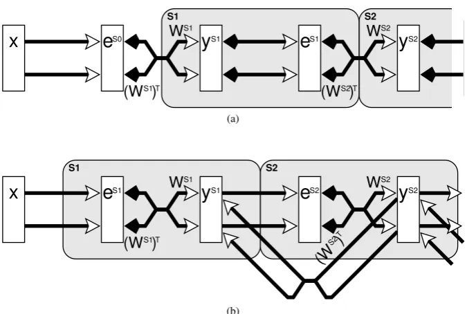
Figure 1:(a) A simplified diagram of the predictive coding model as implemented byRao and Ballard
(1999). (b) The predictive coding model reformulated as a form of biased competition model. Rectan-gles represent populations of neurons, withylabelling populations of prediction nodes andelabelling populations of error-detecting neurons. Open arrows signify excitatory connections, filled arrows indi-cate inhibitory connections, crossed connections signify a many-to-many connectivity pattern between nodes in two populations, parallel connections indicate a one-to-one mapping between the nodes in two populations, and large shaded boxes, with rounded corners, indicate the proposed mapping of the model onto different cortical areas or processing stages.
A neural network implementing equations4 and5 is shown in Figure1b. The substitution ofeSi into the
equation forySihas the effect of modifying the mechanism used to enable the activity in one population ofyunits
to enhance the activity of nodes in the preceding population ofyunits. The original model employed a two stage inhibitory feedback pathway (via theeneurons) from theypopulation in one stage to that in the preceding stage. In contrast, the reformulated model produces a mathematically identical result using direct excitatory feedback from one population of prediction nodes to the preceding one. The re-labelling of the error-detecting nodes has the effect of shifting the assignment of neural populations to processing stages and hence changes the proposed mapping of the algorithm onto cortical regions (as illustrated by the large shaded boxes, with rounded corners, in Figure1). The original PC network (Figure1a) requires feedback from one cortical area to the preceding area to be predominantly inhibitory whereas the reformulated PC architecture (Figure1b) predicts that the effects of cortical feedback are predominately excitatory. The latter is more consistent with cortical physiology (Johnson and Burkhalter,1997;Shao and Burkhalter,1996) and hence the reformulated model proposes the more biologically plausible neural architecture.
Up to this point the model is mathematically identical to the linear model proposed byRao and Ballard(1999): equations4and5are simply equation1re-written in a different form. However, in its current form this model only allows for a straight chain of processing stages, so that each stage receives feedforward input from one preceding stage and feedback from a single subsequent stage. To generalise the model so as to allow more complex hierarchies to be simulated, it is necessary to allow a processing stage to receive inputs from multiple sources. To allow multiple sources of feedforward input, it is simply necessary to replaceySi−1in equation4with a column
vector made of a concatenation of all the feedforward inputs to processing stageSi. These inputs sources could be vectors of node activations calculated at lower-levels in the hierarchy and/or arrays of external inputs.
To allow multiple sources of feedback, equation5needs to be modified. In equation5, feedback excitation received from each individual node in the subsequent stage in the hierarchy is summed to determine the overall top-down excitation received by a prediction node. Hence, feedback from all other possible sources should be treated in exactly the same way (i.e., summed), so that:
ySi←(1−η−ϑ)ySi+ζWSieSi+ηh WSi+1T
ySi+1+ WSzT
ySz+. . .i
Where the term in square brackets is simply the sum of the feedback received from each separate source of
down excitation. These feedback signals can originate from node activations calculated at higher-levels in the hierarchy and/or external inputs.
To include attention in the model, it is assumed that attentional feedback is treated exactly the same as feedback from higher stages in the hierarchy. Only one source of additional feedback to each modelled cortical region is assumed. Specifically, a processing stage (Si) receives attentional feedback from a population of nodes with activations yAi via a set of feedback weights WAiT
. These attentional signals are assumed to arise from circuitry not explicitly modelled here. For convenience, the above equation for ySi is split into two separate
equations, the first (equation7) describing how prediction node activations change with bottom-up stimulation and the second equation (8) describing the top-down influences on the prediction node activations. This results in a final description of the linear model as follows:
eSi=ySi−1− WSiTySi (6)
ySi←(1−η−ϑ)ySi+ζWSieSi (7)
ySi←ySi+ηh WSi+1TySi+1+ WAiTyAii (8)
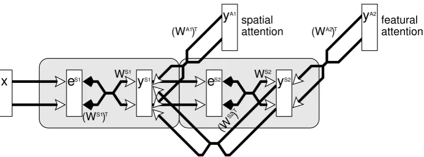
The hierarchical neural network architecture that would implement equations6,7and8is shown in Figure2. This reformulated model can be interpreted as a form of BC model in which cortical regions at neighbouring stages along an information processing pathway are reciprocally connected by excitatory feedforward and feedback connections, and neurons (theypopulation) within each population compete to be active. The outcome of this competition will be influenced by both the bottom-up stimulation received from earlier processing stages and the top-down activation received from higher-levels (including sources of attention). The type of competition used in this reformulated predictive coding model is very similar to that proposed byHarpur and Prager(1996,1994), in which neurons within a region compete via a form of lateral inhibition in which nodes suppress the inputs (rather than the outputs) of other nodes. Specifically, activation from the prediction nodes is fed-back to subtractively inhibit the inputs to those nodes. This calculation of the inhibited input activities is performed in a separate neural population of error-detecting nodes. A similar mechanism of inhibition, in which nodes suppress the inputs to neighbouring nodes, has previously been used to successfully implement a BC model (Spratling and Johnson,
2004). However in this previous model, the inhibition was proposed to take place within the dendrites of the output neurons rather than within a separate, error-detecting, neural population.
The model described by equations6,7and8is mathematically identical to the linear PC model described by
Rao and Ballard(1999) with a minor modification to allow external sources of attention to influence prediction node activities. As discussed in the preceding paragraph, this model can also be interpreted as a form of BC. It will, therefore, be referred to as the linear PC/BC model.
2.3
Introducing Nonlinearities
Up to this point the model is purely linear. In this section two changes to the model will be proposed, both of which introduce nonlinearities. The first modification is to change the mechanism of competition used by replacing equations6and7with:
eSi=ySi−1
+Wˆ Si T
ySi
(9)
ySi← +ySi⊗WSieSi (10)
WhereWSiis a matrix of synaptic weight values normalised such that the sum of each row (i.e., the total weight
received by each node) is equal to one.WˆSiis a matrix representing the same synaptic weight values asWbut
such that the rows are normalised to have a maximum value of one. The parameteris a small constant (i.e., 1×10⁻¹⁰) that prevents division-by-zero errors in the calculation ofeand allows the values ofyto increase from
an initial value of zero, andand⊗indicate element-wise division and multiplication respectively.
The mechanism used in the linear PC/BC model applies subtractive inhibition to the inputs of the prediction nodes. The proposed method employs a mechanism of competition in which nodes divisively modulate their inputs. This is described as ‘divisive modulation’ of the inputs, rather than divisive inhibition, as the values of
x
W
W
A2 T
(W )
S1 T(W )
S1
S2 T
(W )
A1 T(W )
S2
attention
featural
attention
spatial
S1
S1 S2 S2
e
y
e
y
A1 A2
y
y
Figure 2:A simple, two stage, processing hierarchy used in the simulations reported in this article. The symbols used are the same as in Figure1.
(Spratling et al.,2009). An additional advantage of this mechanism is that the values ofeandyare inherently bounded to be non-negative. In contrast, in the linear PC/BC model both error-detecting and prediction nodes are required to be able to signal both positive and negative values. Since biological neurons have firing rates that can never be negative the proposed nonlinear mechanism of competition overcomes a biological implausibility of the linear model.
The second modification is to allow excitatory feedback from one processing stage to the preceding stage to be modulatory rather than additive;i.e., to replace equation8with:
ySi ←ySi⊗1 +ηh WSi+1TySi+1+ WAiTyAii (11)
Cortical feedback has been observed to multiplicatively modulate the bottom-up driven activation of lower-level neurons (Andersen et al.,1985;Brotchie et al.,1995;McAdams and Maunsell,1999;Motter,1993;Treue,
2001;Williford and Maunsell,2006). While these modulatory effects might be brought about by the interplay between linear mechanisms of excitation and inhibition (Reynolds and Chelazzi,2004), several physiological mechanisms have been identified that could allow cortical feedback to have a direct modulatory effect on neural responses (Friston,2005; Larkum et al.,2004; Spruston,2008; Sripati and Johnson,2006). Consideration of computational requirements have also lead to arguments in favour of cortical feedback being modulatory, rather than additive (Crick and Koch,1998;Grossberg and Raizada,2000;Roelfsema,2006), for example, in order to avoid top-down expectation producing strong responses to stimuli for which there is no supporting evidence (i.e., to prevent the “hallucination” of image features that are not present).
The model described by equations9,10and11will be referred to as the nonlinear PC/BC model. This model can also be implemented using the neural architecture shown in Figure2.
3
Results
To demonstrate that predictive coding can be used to model cortical biased competition both the linear PC/BC model (equations6,7 and8) and the nonlinear PC/BC model (equations9,10 and11) were used to simulate empirical data associated with attention. A simple two-stage hierarchy, as illustrated in Figure2, was used in all simulations. These two processing stages are assumed to correspond to two neighbouring cortical regions along the ventral pathway. The lower region received input from a more peripheral cortical or thalamic region (that was not explicitly modelled) and each processing stage could receive attentional signals (also assumed to arise from circuitry not explicitly modelled here).
For experiments on spatial attention it was assumed that differential feedback would be received by ventral regions with RFs at an appropriate scale to define the attended region. Hence, attention to the spatial location occupied by one stimulus would preferentially enhance the response of the corresponding node representing that stimulus in the lower stage of the hierarchy. In contrast, for object-based attention it was assumed that feedback signals are received by nodes higher up the ventral pathway which are selective to the attended objects. Hence, attention to a feature is modelled by a top-down signal that enhances the response of a node encoding that feature in the second stage of the hierarchy.
3.1
Selective Attention
The first three experiments simulate the effects of selective attention (both spatial and featural) on the response properties of single cells. In each simulation, the neural populations in both the first and second processing stages contained only two nodes, and the input to the hierarchy came from two inputs (hencen=m= 2for each processing stage). Similarly simple networks containing only a few nodes, employing different implementations of BC, have previously been used to simulate some of the same data modelled here (Deco and Rolls,2005;Reynolds et al.,1999;Spratling and Johnson,2004). In each experiment the response of one node in the upper region of the hierarchy was recorded (yS2
1 ). This node received bottom-up stimulation (via the error-detecting nodes) from
two prediction nodes in the preceding stage of the hierarchy. One of these lower-level prediction nodes provided strong stimulation to the recorded node, while the other provided weaker input. Hence, the recorded node could be strongly activated by a preferred stimulus and weakly activated by a poor stimulus.
The prediction nodes in the first stage of the hierarchy were assumed to have smaller, non-overlapping, RFs that were selective to two different input stimuli. The total synaptic weight received by each node was normalised
to equal one. Hence, the weight matrix for the first stage was set to the identity matrix,i.e.,WS1=
1 0 0 1
.
Thus, one lower-level prediction node was exclusively selective to the preferred stimulus of the recorded, higher-level, prediction node while the other lower-level prediction node was activated by the poor stimulus for the recorded node. Since the mechanism of competition used here causes one node to inhibit an input to another node in proportion to the bottom-up weight received from that input by the inhibiting node, nodes in the first hierarchical stage did not compete because their afferent synaptic weights were non-overlapping. The weight matrix for the
second processing stage had the form:WS2=
w1 1−w1
1−w2 w2
. Wherew1andw2were parameters to be
fitted to the data.
Since the model was being used to simulate neurophysiological data collected from different cells with distinct selectivities, different sets of weight values were used in the different simulations. The weight values that provided the best fit to the experimental data were found by systematically varyingw1andw2in the following ranges. For
w1values of 0.6, 0.7, 0.8 and 0.9 were used. These values all exceed 0.5 since it is required that the recorded
node be more responsive to the preferred stimulus than the poor stimulus. Forw2values of 0.1, 0.3, 0.5, 0.7, and
0.9 were used. For each combination of weights the parameterηwas also varied between 0.1 and 0.9 in steps of 0.2. Additionally, for the linear model the parametersζandϑwere varied between 0 and 1 in steps of 0.25. An exhaustive search of all these possible parameter combinations was performed for each algorithm and parameters that provided a good subjective fit to the physiological data were chosen.
The two matrices of attentional weights were set to the identity matrix,i.e.,WA1=WA2=
1 0 0 1
. All
values in the the vectorsyA1 andyA2were set to zero except when simulating experimental conditions where
attention was required, in which case the corresponding element in the vectoryA1oryA2was set equal to one.
In all experiments, 20 iterations of the linear and nonlinear PC/BC models were performed for each experi-mental condition. The elements ofx(the sensory input) were set to a value ofxor0to reflect the presence or absence of a stimulus. The value ofxwas set equal to the fractional Michelson contrast used for the presentation of stimuli in the corresponding empirical experiment, if this value was reported. A value ofx= 0.65was used in all other cases. The sensory input was reset to zero after 13 iterations, to simulate the offset of the stimuli used in the physiological experiments.
3.1.1 Spatial Selectivity
For neurons in the ventral pathway the response to a stimulus, that generates a strong response when presented in isolation, is reduced by the introduction of a second, non-preferred, stimulus within the RF (Reynolds et al.,1999). Hence, rather than being processed independently, multiple stimuli, within the same RF, appear to compete in a mutually suppressive manner (Kastner and Ungerleider,2000). If attention is directed toward one stimulus then the response becomes more similar to the response that would be generated by that stimulus in isolation (Luck et al.,1997a;Moran and Desimone,1985;Reynolds et al.,1999). Hence, attention appears to bias the competition in favour of the attended stimulus. These effects are illustrated in Figure3a which shows the response of a single cell recorded in area V2. Similar results have been demonstrated for cells in area V4, inferior temporal cortex, in area MT of the dorsal pathway, and in prefrontal cortex (Everling et al.,2002;Moran and Desimone,1985;
Reynolds et al.,1999;Reynolds and Desimone,1999;Treue and Martinez-Trujillo,1999).
Response
Time
pref attend away poor attend away pair attend away pair attend pref
(a) Empirical data
Time
Response
(b) Linear PC/BC
Time
Response
(c) Nonlinear PC/BC
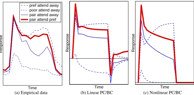
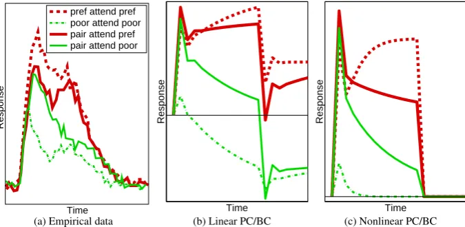
Figure 3:The effect of spatial attention on the response of a neuron. Responses are shown for different combinations of stimuli appearing within the RF of a single neuron. (a) The response of a cell in V2 (adapted fromReynolds et al.,1999). (b) Simulation results for the linear PC/BC model. (c) Simulation results for the nonlinear PC/BC model. For (a) the response was measured in spikes per second and time in milliseconds, for (b) and (c) response and time are in arbitrary units and have been scaled to resemble (a). The value of zero on the y-axis is indicated by the x-axis in (a) and by the thin horizontal lines in (b) and (c).
stimulus in isolation. Results for simulations with the linear PC/BC model and the nonlinear PC/BC model are shown in Figures3b and 3c respectively. These results were obtained with parameters w1 = 0.9,w2 = 0.5,
η = 0.2,ζ = 1, andϑ= 0for linear PC/BC, andw1 = 0.8,w2 = 0.5andη = 0.3for nonlinear PC/BC. The
empirical data was recorded using stimuli presented at a Michelson contrast of 86%, hence,x= 0.86was used for the stimuli presented to the model. The thin horizontal lines in Figures3b and3c indicate a response of zero. It can be seen that linear PC/BC allows negative responses. However, it is possible to clip the outputs of the prediction nodes at zero to prevent negative activities, and this has very little effect on the positive part of the graph shown in Figure3b. It can be seen that both versions of the PC/BC model generate responses (after the initial transient response) that are qualitatively similar to those of the empirical data. In both cases, when the preferred stimulus of the recorded node was presented to the network, the recorded node quickly won the competition to respond to this stimulus and produced a high output. In contrast, when the poor stimulus was presented in isolation, the other node in the second processing stage won the competition and suppressed the response of the recorded node so that it generated a weak and brief output to its non-preferred stimulus. When both stimuli were present, both prediction nodes in the second processing stage were strongly activated and there was on-going competition between them which partially suppressed both responses. Hence, the response of the recorded node to the pair of stimuli was less than its response to its preferred stimulus in isolation. Attention to the preferred stimulus in the pair resulted in an enhanced response from the prediction node in the first processing stage which represents the preferred stimulus. This elevated feedforward activation in turn produced a stronger response from the recorded node in the second processing stage.
3.1.2 Spatial Selectivity and Contrast
The effect of attention in the previous simulation was to change the strength of the response of one of the prediction nodes in the first processing stage and hence to enhance the bottom-up activation received by the second processing stage. A similar effect could be achieved if the response of the node in the first stage was affected by changing the stimulus contrast. Hence, in the linear and nonlinear PC/BC models, a strong bottom-up signal could bias competition in just the same way as a top-down signal can. The interplay between attention and stimulus saliency has been explored experimentally (De Weerd et al.,1999;Kastner and Ungerleider,2000;Martinez-Trujillo and Treue,2002;Reynolds and Chelazzi,2004;Reynolds and Desimone,1999,2003;Reynolds et al.,2000;Vecera,
2000).
One experiment investigating the interaction between stimulus contrast and spatial selective attention (Reynolds and Desimone,2003) is very similar to that described in Section3.1.1, but with the contrast of the poor stimulus being varied. Specifically, the firing rates of V4 cells were measured when a preferred and a poor stimulus were presented within the recorded cell’s RF. The stimuli were presented individually and as a pair when attention was directed to a location outside the RF. The response to the pair of stimuli was also recorded when attention was
directed to the poor stimulus. The experiment was repeated for different poor stimulus contrasts (typically 5%, 10%, 20%, 40% and 80% Michelson contrast) but with a fixed contrast for the preferred stimulus (typical 40% Michelson contrast). The results are shown in Figure4a.
It can be seen that, as the contrast of the poor stimulus increases (from left to right in Figure4a), the response elicited by this stimulus in isolation increases. However, counter-intuitively, the response to the pair of stimuli decreases as the contrast of the poor stimulus increases. In other words, the suppression caused by the poor stimulus increases with contrast, when the pair of stimuli are presented, but the excitation of the poor stimulus increases with contrast, when it is presented in isolation. Attention to the poor stimulus has the effect of increasing the suppression of the response to the pair of stimuli. These results were simulated using the linear and nonlinear PC/BC models and the results are shown in Figures4b and4c. These results were obtained with parameters
w1 = 0.9,w2 = 0.6,η = 0.2,ζ = 1, andϑ = 0for linear PC/BC, andw1 = 0.9,w2 = 0.7andη = 0.5for
nonlinear PC/BC. It can be seen that the sustained responses generated by both models successfully accounts for the empirical data. Again, the negative responses of the linear model can be removed by simply taking the positive half-rectified values of the prediction node activations, with little impact on the positive portion of the response.
In both models, when the preferred stimulus of the recorded node is presented to the network, the recorded node quickly wins the competition to respond to this stimulus and produces a strong response. Since the contrast of the preferred stimulus was constant, the recorded response was the same in each experimental condition. In contrast, when the poor stimulus is presented in isolation, the other node in the second processing stage wins the competition and suppresses the activity of the recorded node so that it generates a weak and brief response to its non-preferred stimulus. The size of this brief response increases with the contrast of the poor stimulus as the bottom-up activation received by the recorded node, before it is inhibited by the other node, increases.
When both stimuli are present at high contrast, both prediction nodes in the second processing stage are strongly activated and there is on-going competition between them which partially suppresses both responses. Hence, the response of the recorded node to the pair of stimuli is less than its response to its preferred stimulus in isolation. However, when the poor stimulus is presented at low contrast, the activation of the second stage prediction node which represents the poor stimulus is weaker, and hence the suppression to the recorded node also weakens. At very low contrast, the bottom-up activation from the poor stimulus is so weak that it has very little effect on the responses of either node in the second processing stage and hence the recorded response becomes similar to that recorded when the preferred stimulus appears in isolation. Attention to the poor stimulus in the pair results in an enhanced response from the prediction node in the first processing stage which represents the poor stimulus. This elevated feedforward activation in turn produces a stronger response from the non-recorded node in the second processing stage. This node can therefore more strongly inhibit the recorded node’s response, and hence the suppressive effect of the poor stimulus is enhanced by attention.
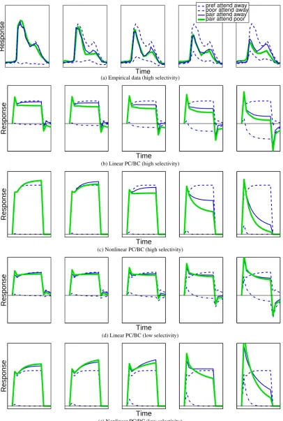
A second counter-intuitive result from the empirical data is that a node which is more selective for the pre-ferred stimulus (i.e., a node that generates a weaker response to the poor stimulus in isolation) is subject to a greater suppression in its response to the preferred stimulus when this is presented together with the poor stimulus (Reynolds and Desimone,2003). In other words, the poorer the poor stimulus the weaker the response elicited by the pair of stimuli. Both the linear and nonlinear PC/BC models also show this effect. Response histograms for a population of V4 cells that were highly selective to the preferred stimulus are shown in Figure4a and the simulations of this data are shown in Figure4b and4c. Reynolds and Desimone(2003) also analysed a second population of less selective cells (however, response histograms of this data were not produced). This less selec-tive population was modelled by reducing the value of the parameterw1to make the recorded node less selective
for the preferred stimulus. Figure4d shows results for the linear model withw1 = 0.7and Figure4e shows this
result for the nonlinear model withw1 = 0.7. All other parameters were unchanged in both cases. Comparing
Figure4d with Figure4b and Figure4e with Figure4c it can be seen that the suppression due to the poor stimulus (at high contrasts) is increased when the recorded node is highly selective.
Two effects give rise to this result. Firstly, because the synaptic weight from the preferred input is larger the response to the preferred stimulus in isolation is enhanced resulting in suppression becoming greater when the poor stimulus is present relative to the preferred stimulus in isolation (this effect is most pronounced in the nonlinear model). Secondly, the response to the pair of stimuli is decreased in absolute terms between medium and highly selective nodes. The reduction in response to the pair of stimuli is a result of the competition between the recorded node and the other node in the second processing stage. As the recorded node becomes more selective to one stimulus, it becomes a poorer representation of the pair of stimuli. The other node, which does provide a good representation of the pair, thus wins the competition more quickly and more rapidly suppresses the activation of the recorded node. This effect is due to the particular form of competition used in the PC/BC model, in which nodes compete to receive inputs rather than to generate outputs. This enables patterns of pre-synaptic activity to be parsed into accurate representations, even when those representations overlap (Harpur and Prager,1996,1994;
Time
pref attend away poor attend away pair attend away pair attend poor
Response
(a) Empirical data (high selectivity)
Response
Time
(b) Linear PC/BC (high selectivity)
Response
Time
(c) Nonlinear PC/BC (high selectivity)
Response
Time
(d) Linear PC/BC (low selectivity)
Response
Time
(e) Nonlinear PC/BC (low selectivity)
Highly
Selecti
v
e
−0.3 −0.25 −0.2 −0.15 −0.1 −0.05 0 0.05
low high
Attention Modulation Index
Contrast of poor stimulus
−0.3 −0.25 −0.2 −0.15 −0.1 −0.05 0 0.05
low high
Attention Modulation Index
Contrast of poor stimulus
−0.3 −0.25 −0.2 −0.15 −0.1 −0.05 0 0.05
low high
Attention Modulation Index
Contrast of poor stimulus
Less
Selecti
v
e
−0.3 −0.25 −0.2 −0.15 −0.1 −0.05 0 0.05
low high
Attention Modulation Index
Contrast of poor stimulus
(a) Empirical data
−0.3 −0.25 −0.2 −0.15 −0.1 −0.05 0 0.05
low high
Attention Modulation Index
Contrast of poor stimulus
(b) Linear PC/BC
−0.3 −0.25 −0.2 −0.15 −0.1 −0.05 0 0.05
low high
Attention Modulation Index
Contrast of poor stimulus
(c) Nonlinear PC/BC
Figure 5:Quantitative data showing the effect of spatial attention with changing contrast. Each sub-plot shows values of the attention modulation index (AMI) for varying poor stimulus contrasts. The top row shows the results when neurons are highly selective to the preferred stimulus, and the bottom row shows results for neurons which are less selective to the preferred stimulus. Column (a) shows the average AMI values for a population of cells in V4 (Reynolds and Desimone,2003). Column (b) shows simulation results for the linear PC/BC model. Column (c) shows simulation results for the nonlinear PC/BC model.
case, (Figure4d and Figure4e) attention to the poor stimulus causes little additional suppression of the response to the pair, but in the high selectivity case (Figure4b and Figure4c), attention to the poor stimulus causes additional suppression to the response to the pair. This is also consistent with the empirical data (Reynolds and Desimone,
2003).
As well as providing a good qualitative fit to the data, both models also provide a good quantitative fit.
Reynolds and Desimone (2003) report the response, averaged over time, generated by the preferred stimulus presented in isolation and the average response generated by the pair of stimuli when presented at equal contrasts. In the population of cells that are highly selective for the preferred stimulus the response to the preferred stimulus is 46% higher than the response to the pair (29.5 spikes/s compared to 20.2 spikes/s). In the low selectivity popula-tion these average responses are much more similar (39.3 spikes/s compared to 36.5 spikes/s). In the linear model, when the recorded node has high selectivity the response to the preferred stimulus is 45% higher than the response to the pair (0.32 compared to 0.22), whereas the responses are similar when the recorded node has low selectivity (0.32 compared to 0.30). In the nonlinear model, the response to the preferred stimulus is 39% higher that the response to the pair in the high selectivity case (0.43 compared to 0.31) whereas these responses are similar in the low selectivity case (0.31 compared to 0.33). The average responses in the simulations were recorded from the first iteration following the transient response (iteration 4) until the offset of the stimulus (iteration 13).
Reynolds and Desimone(2003) also report the size of the attentional effect, in terms of an attentional modula-tion index (AMI), for both the high and low selectivity populamodula-tions across all poor stimulus contrasts. The AMI is calculated as Rpp−Rpa
Rpp+Rpa, whereRppis the time averaged response to the pair of stimuli when attention is directed to the poor stimulus, andRpais the time averaged response to the pair of stimuli when attention is directed away.
The spike counts for the V4 cells were averaged over the same time interval as that used to calculate the average responses reported in the previous paragraph. The same time interval, as used previously, was therefore also used to calculate the AMI values for the simulated data. The AMI values averaged across the high and low selectivity sub-populations of V4 cells are shown in Figure5a. The AMI values calculated from the simulations are shown in Figure5b for the linear model, and Figure5c for the nonlinear model. It can be seen that there is good agreement between both models and the empirical results.
3.1.3 Featural Selectivity
pair attend poor pref attend pref poor attend poor pair attend pref
Response
Time (a) Empirical data
Time
Response
(b) Linear PC/BC
Time
Response
(c) Nonlinear PC/BC
Figure 6:The effect of featural attention on the response of a neuron. Responses are shown for different combinations of stimuli appearing within the RF of a single neuron. (a) The averaged response for a pop-ulation of cells in V4 (adapted fromChelazzi et al.,2001). (b) Simulation results from the linear PC/BC model. (c) Simulation results from the nonlinear PC/BC model. For (a) the response was measured in spikes per second and time in milliseconds, for (b) and (c) response and time are in arbitrary units and have been scaled to resemble (a). The value of zero on the y-axis is indicated by the x-axis in (a) and by the thin horizontal lines in (b) and (c).
were measured from cells in area V4, with RFs sufficiently large to encompass the stimulus array. Different responses were generated when the target object was the preferred stimulus of the recorded cell compared to when the target was a non-optimal stimulus (see Figure6a). Results are similar to those for attentional selection using spatial cues (Section 3.1.1) in that when the stimulus array contains a pair of objects the response of the cell becomes more similar to the response that would be generated by the attended stimulus in isolation.
The simulation results for this experiment are shown in Figures6b and6c. These results were obtained with parametersw1 = 0.8,w2 = 0.3,η = 0.1,ζ = 1, andϑ = 0for linear PC/BC, andw1 = 0.8,w2 = 0.5and
η= 0.1for nonlinear PC/BC. Following the initial transient response, both models provide a qualitative fit to the experimental data (if the negative response in the linear model are ignored). In the previous simulations, attention targeted the first processing stage in the hierarchy. In this simulation, attentional signals provided top-down bias to nodes in the second processing stage.
When a single stimulus is presented to the network the node in the second processing stage with the preference to that stimulus wins the competition and inhibits the other node from generating an output. Hence, the recorded node wins the competition for its preferred stimulus and generates a strong response, but loses the competition to represent the poor stimulus and has its response suppressed. When both stimuli are presented, there is ongoing competition between the two nodes in the second processing stage. This partially suppresses the response of both nodes. However, if attention is directed to the recorded node, this enhances the response of the recorded node and overcomes some of the suppression due to competition. In contrast, when attention targets the other node in the second processing stage, this node has its response elevated which results in the response of the recorded node being more strongly suppressed via competition.
3.2
Attention and Tuning
The next two experiments simulate the effects attention on the tuning response functions of single cells. As in the previous experiments a two-stage model (as illustrated in Figure2) was employed. Also, as in previous simulations, the matrixWS1 was made equal to the identity matrix, so that nodes in the first processing stage
effectively had non-overlapping RFs, and two matrices of attentional weights (WA1 andWA2) were also set
equal to the identity matrix so that attentional biases could be selectively directed to individual nodes. All values in the the vectorsyA1andyA2were set to zero except when simulating experimental conditions when attention
was required. As previously, experiments concerning spatial attention, used feedback targeting the prediction nodes in the first stage, while experiments on featural attention employed attentional signals targeting the second processing stage. Parameter values were set equal to the median values of those found to provide the best fits to the experimental data modelled in Section3.1(i.e.,η = 0.2,ζ= 1,ϑ= 0for the linear model, andη = 0.3for the nonlinear model).
Response
Orientation
(a) Empirical data
Response
Orientation
(b) Linear PC/BC
Response
Orientation
(c) Nonlinear PC/BC
Figure 7:The effect of spatial attention on the tuning response function of a neuron. Response strength is shown for varying stimulus orientation when attention is directed to the location occupied by the stimulus (circular markers) and when attention is directed away from the stimulus (square markers). (a) Experimental results (adapted from McAdams and Maunsell,1999) showing the average tuning curve measured in V4. Simulation results for (b) the linear PC/BC model and (c) the nonlinear PC/BC model. The x-axis in (a) corresponds to the spontaneous response level of the recorded cells, the thin horizontal lines in (b) and (c) corresponds to a response of zero in the simulation.
In contrast to previous simulations, each prediction node in the second processing stage received a set of synaptic weights that had a Gaussian profile. Nodes in the first stage were assumed to represent either a stimulus orientation or a direction of motion. Hence, each second stage node had a preferred orientation/direction but was broadly tuned to a range of inputs. Nine nodes, with different preferred inputs, were used in the second processing stage so that the preferred inputs were equally distributed between0and180oin the case of orientation preference, and0and360oin the case of direction of motion preference. The input stimulation (x) received by the first processing stage also had a Gaussian profile. The variance of the input and the weights were tuned separately for the linear and nonlinear models to obtain a good fit to the empirical data.
3.2.1 Spatial Facilitation and Tuning
The effects of spatial attention on the orientation tuning of cells in areas V1 and V4 was investigated byMcAdams and Maunsell(1999). In this experiment a single orientation grating was presented within the RF of the recorded cell. It was found that when attention was directed to the location of the orientation grating the cell’s response was enhanced compared to when attention was directed to a different location. By varying the orientation of the stimulus relative to the recorded cell’s preferred orientation, tuning curves were generated for both the attended and non-attended conditions (see Figure7a). The effect of attention was a multiplicative scaling of the tuning response function.
To simulate this experiment, the response of one node in the second processing stage was measured to varying input orientations, both with and without attention. In the attended condition all nodes in the first processing stage received equal top-down activation (i.e., all values in the vectoryA1were made equal to one). This means that attention was feature independent (i.e., spatial) as it targeted equally all the nodes in the first processing stage. Results for the linear and nonlinear PC/BC model are shown in Figure7b and 7c respectively. It can be seen that in the linear model attention produces an upward translation of the orientation tuning curve. This is due to each prediction node in the first processing stage receiving an equal, additive, top-down excitation that is fed-forward to equally enhance the response of the recorded node irrespective of the orientation of the stimulus. In contrast, the nonlinear model produces a result similar to the empirical data. This is due to the multiplicative effect of the top-down input to the prediction nodes in the first processing stage, which means that the feedforward excitation received by the recorded node is enhanced in proportion to the match between the orientation of the stimulus and the preferred orientation of the node. Note that the model does not simulate spontaneous neural activity and hence at the null orientation the response of the recorded node approaches zero. In contrast, the neural response in the physiological data remains above zero and this spontaneous activity is multiplicatively modulated by attention.
3.2.2 Featural Facilitation and Tuning
Response
Direction (a) Empirical data
Response
Direction
(b) Linear PC/BC
Response
Direction
(c) Nonlinear PC/BC
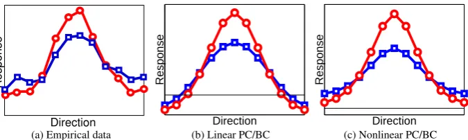
Figure 8: The effect of featural attention on the tuning response function of a neuron. Responses are shown for varying directions of motion when attending the same direction of motion as the stimulus (cir-cular markers) and when attending a stationary fixation point (square markers). (a) Experimental results (adapted fromMartinez-Trujillo and Treue,2004) showing the response of an MT neuron. Simulation results for (b) the linear PC/BC model and (c) the nonlinear PC/BC model. The value of zero on the y-axis is indicated by the x-axis in (a) and by the thin horizontal lines in (b) and (c).
direction of motion was ignored). In the second condition attention was directed to a second moving random dot pattern outside the RF of the recorded neuron which had the same direction of motion as the pattern within the recorded cell’s RF (i.e., attention was directed to the same direction of motion as the stimulus). It was found that attention caused an enhancement of the cell’s response when the direction of motion was close to the preferred direction for the cell, but a suppression of response when the direction of the stimulus (and hence the attended direction) was far from the cell’s preferred direction (see Figure8a).
To simulate this experiment, the response of one node in the second processing stage was measured to varying input directions, both with and without attention. In the attended condition nodes in the second processing stage received top-down activation that had a Gaussian profile centred on the direction of motion of the input stimulus. Results for the linear and nonlinear PC/BC model are shown in Figure8b and8c respectively. It can be seen that both versions of the model simulate the multiplicative response enhancement that occurs for directions of motion similar to the preferred direction of motion for the recorded node. This is because the attentional signal received by the recorded node in the second processing stage increases in proportion to the match between the attended direction and the preferred direction of the node. Furthermore, both the linear and nonlinear models show response suppression when the direction of motion is dissimilar to the preferred direction. This is caused by the competition that occurs between the prediction nodes in the second processing stage. When the input stimulus is dissimilar to the preferred stimulus of the recorded node, it is more similar to the preferred input of other nodes. These other nodes win the competition and suppress the input received by the recorded node, reducing its response. When featural attention enhances the response of the winning node, this results in an even greater suppression of the recorded node’s response.
3.3
Attention and Behaviour
The effects of attention have also been extensively studied using behavioural measures. A particularly influential experimental procedure (Posner,1980) employs a cue to direct covert attention to one of two spatial locations where a subsequently presented target is most likely to appear. Numerous variations on this paradigm (e.g.,
Posner,1980;Vossel et al.,2006;Wright et al.,1995) show the same pattern of results: faster reaction times when the cue is valid meaning that the target appears at the cued location, and slower reaction times when the cue is invalid so that the target appears at the uncued location. Furthermore, the strength of the effect is dependent on the proportion of trials for which the cue is valid (Vossel et al.,2006). Typical reaction time data are shown in Figure9a for an experiment in which participants had to detect the onset of the target (irrespective of location) following a central cue .
The PC/BC model was used to provide a very simple simulation of this experiment. The first processing stage consisted of two prediction nodes, with non-overlapping RFs (i.e.,WS1 was a 2 by 2 identity matrix).
These nodes acted as feature detectors for the target stimulus at the two locations. Both prediction nodes in the first processing stage provided input to a second processing stage that contained only a single prediction node (WS2= [0.5,0.5]). This node responded (equally, in the absence of top-down bias) to the target at either location.
Reaction time was presumed to be inversely proportional to the strength of the response of the prediction node in the second processing stage (i.e., simulated reaction time= 1−yS2
1 ). This is equivalent to using the ‘race’ model
of decision making. Attention was directed to the prediction nodes in the first processing stage (WA1 was an
identity matrix). This is consistent with empirical data suggesting that the attentional cue enhances early sensory
0.2 0.5 0.8
Reaction Time
Cue Validity
(a) Empirical data
0.2 0.5 0.8
1−Response
Cue Validity
(b) Linear PC/BC
0.2 0.5 0.8
1−Response
Cue Validity
(c) Nonlinear PC/BC
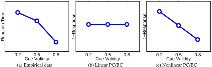
Figure 9: The effect of spatial attention on reaction time. (a) Experimental results (fromWright et al.,
1995) showing the mean reaction times as a function of cue validity. Simulation results for (b) the linear PC/BC model and (c) the nonlinear PC/BC model.
processing (Wright et al.,1995). The strength of the attention signal was made equal to the prior probability that the target would appear at each location. Hence, in an experiment in which the cue accurately predicted the location of the target on 80% of trials, and the cue pointed to location 1, thenyA1 = [0.8,0.2]T. All parameter
values were identical to those used in the Section3.2. Results from the simulation are shown in Figure9b for the linear model, and Figure9c for the nonlinear model.
It can be seen that for the linear PC/BC model, the reaction time is constant in all conditions. This is due to the prediction nodes in the first processing stage receiving additive top-down stimulation from the attention signals. The total top-down activation received by the two nodes in the first processing stage is equal in each condition, and hence the total feedforward activation received by the prediction node in the second processing stage is constant. In contrast, the nonlinear PC/BC model is able to simulate the empirical data. In this case the attentional feedback is modulatory and hence it only affects the activation of one node in the first processing stage corresponding to the location where the target appears. If this location was cued, then the attention signal will strongly enhance the response of this node and hence increase the feedforward activation sent to the prediction node in the second processing stage. In contrast, if the location where the target appears was not cued, attention will only weakly enhance the response of the node in the first processing stage, resulting in less feedforward stimulation of the second processing stage.
3.4
Feature Binding
Selective attention has been proposed to play an important role in solving the binding problem (Luck and Ford,
1998;Luck et al.,1997b;Reynolds and Desimone,1999;Treisman,1998;Treisman and Gelade,1980), particu-larly in resolving the ambiguous assignment of features to objects when multiple stimuli are processed simultane-ously (Luck et al.,1997b).
The empirical data described in the previous sections (particularly for selective attention, Section3.1) demon-strates that the responses of cortical neurons are dominated by the attended (or most salient) stimulus within their RFs and, hence, that attended (or salient) information is preferentially selected for transmission to subsequent cortical regions for further processing. The BC hypothesis proposes that this selection of relevant information is achieved via competition between neurons representing attended and non-attended stimuli. Neurons which represent the attended (or most salient) stimulus receive enhanced activation from top-down attention signals (or salient, bottom-up, stimulus attributes). This enhanced activation biases these neurons to succeed in the compe-tition to be active, and enables these neurons to inhibit other cells that do not represent the attended (or salient) stimulus. Hence, information about the attended (or most salient) stimulus is more strongly represented and trans-mitted to subsequent processing stages. Even if the competition does not lead to the complete suppression of neural responses encoding irrelevant information, the enhancement to the firing rate of neurons encoding the at-tended stimulus will cause them to be preferentially processed and can be seen as a ‘label’ for relevant information (Roelfsema,2006;Roelfsema et al.,2000).
3.4.1 Binding Feature Conjunctions via Featural Attention
B R 0 90 B−0 B−90 R−0 R−90 B R 0 90 B−0 B−90 R−0 R−90 B R 0 90 B−0 B−90 R−0 R−90 B R 0 90 B−0 B−90 R−0 R−90 B R 0 90 B−0 B−90 R−0 R−90 B R 0 90 B−0 B−90 R−0 R−90
(a) Linear PC/BC
B R 0 90 B−0 B−90 R−0 R−90 B R 0 90 B−0 B−90 R−0 R−90 B R 0 90 B−0 B−90 R−0 R−90 B R 0 90 B−0 B−90 R−0 R−90 B R 0 90 B−0 B−90 R−0 R−90 B R 0 90 B−0 B−90 R−0 R−90
(b) Nonlinear PC/BC
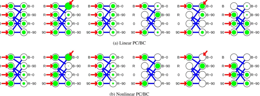
Figure 10: The effects of selective object-based attention on feature binding in a simple task simulated with (a) the linear PC/BC model, and (b) the nonlinear PC/BC model. Each subplot shows the responses of the prediction nodes in the first and second processing stages to different combinations of input stimuli and attentional states. The strength of each node’s response (at the end of 20 iterations) is indicated by the diameter of the shading. Four prediction nodes in the first processing stage represent independent features of the input stimulus. The four prediction nodes in the second processing stage represent pairwise conjunctionsof the features represented in the first stage. Connections between the processing stages correspond to the synaptic weights inWS2and hence show the weights received by the prediction nodes
in the second stage from the outputs of prediction nodes in the first stage via the error-detecting nodes (not shown). The connections also indicate the feedback weights received by the prediction nodes in the first stage from the prediction nodes in the second stage. Horizontal arrows indicate which nodes receive bottom-up stimulation, while arrows oriented diagonally indicate nodes that receive attentional input. Note that for each condition, the external inputs to both models are identical. The difference between (a) and (b) in the activities of the prediction nodes in the first processing stage is a result of the different effects of top-down bias between the two models.
object, and which are attributes of other objects. For example, if neurons encoding the colours blue and red, and the orientations 0 and 90 are all simultaneously active, is this due to the presentation of a red-vertical line and a blue-horizontal line or to a red-horizontal line and a blue-vertical line (Rosenblatt,1961;Thorpe,1995;von der Malsburg,1995)?
The PC/BC model can be used to simulate this ambiguous situation. The parameters used were the median values of those found to provide the best fits to the data modelled in Section 3.1and hence the same as the parameters used in the simulations described in Sections3.2and3.3. Four nodes in the first processing stage were used to represent the individual features blue (‘B’), red (‘R’), horizontal (‘0’) and vertical (‘90’), while four nodes in the second processing stage each received inputs from a different combination of two nodes in the lower level so that they represented the conjunctions blue-horizontal (‘B-0’), blue-vertical (‘B-90’), red-horizontal (‘R-0’), and red-vertical (‘R-90’). For both the linear and nonlinear versions of the model, when every node in the first processing stage received bottom-up stimulation, all the nodes in the second stage became partially, and equally, active (Figure10first column). The nodes were more weakly active than the winning node when the input was unambiguous (i.e., when it consisted of only one colour and one orientation feature, as in the fourth column of Figure10). For the linear model, nodes in the ambiguous case were active with 75% of the strength of the winning node in the unambiguous case. In the nonlinear model, nodes in the ambiguous case were active with 50% of the strength of the winning node in the unambiguous case. This behaviour could be interpreted in probabilistic terms as saying that each conjunction is predicted to be present in the input with a probability less than in the unambiguous case. The nonlinear model correctly divides the probability in half.
Attentional feedback can resolve the ambiguity in the sensory data by providing bias for one possible inter-pretation over all others. For example, if attention targets the node in the second processing stage that represents ‘B-0’ then this will enhance this node’s activation and cause it to be most active (Figure10second column). Fur-thermore, due to the form of competition used in the model, enhancing the activation of node ‘B-0’ will cause it to more strongly inhibit the inputs received by other second stage nodes from features ‘B’ and ‘0’. This will reduce the response of nodes representing overlapping conjunctions (i.e.,’B-90’ and ‘R-0’) but it will not inhibit the inputs to node ‘R-90’. Hence, top-down bias in favour of one conjunction of features will also cause a strong
response from the node representing the complementary conjunction, and hence both nodes compatible with the biased interpretation produce a strong response (i.e., binding together blue and horizontal also results in red and vertical being bound).
Rather than using attention to resolve the ambiguity, it is also possible to bias the competition using bottom-up factors. If the second stage node representing ‘B-0’ had stronger weights than the other nodes (perhaps due to more prior experience with this conjunction having lead, via activity-dependent learning, to a more selective repre-sentation), then this will lead to ‘B-0’ winning the competition due to it receiving stronger bottom-up stimulation. Similarly, if the features ‘B’ and ‘0’ are presented at a higher contrast, then this will lead to the node representing this conjunction receiving stronger feedforward activation and hence being the most active node (see Figure10
column 3). In this particular example, inputs ‘B’ and ‘0’ are 30% stronger than inputs ‘R’ and ‘90’. This leads to the node representing the conjunction ‘B-0’ having a response that is 22% higher than any other node in the linear model, and a response 32% higher in the nonlinear model.
The conditions shown in the fifth and sixth column of Figure 10illustrate limitations of the linear PC/BC model. Firstly, when attention is directed to an object that is not present in the input, then this can lead to the wrong parsing being generated. In this example, the input is unambiguous consisting of only one colour (‘B’) and one orientation (‘90’). Without attention this is represented by the appropriate node in the second processing stage (Figure10fourth column). When attention is directed to the second stage node that represents the conjunction ‘B-0’ (Figure10fifth column), this has no effect in the nonlinear model, but results in the attended node producing the strongest response in the linear model. The additive feedback in the linear model causes attention to be able to ‘hallucinate’ objects that are not present in the input. In contrast, the multiplicative feedback used in the nonlinear model only allows attention to enhance the responses of neurons that are driven by bottom-up activation.
The sixth column of Figure10illustrates a situation where multiple objects sharing a feature are present in the input (e.g., two red bars, one with an orientation of 0 degrees and the other at 90 degrees). The nonlinear PC/BC model resolves the competition between the nodes in the second processing stage so that the nodes representing the conjunctions ‘R-0’ and ‘R-90’ are active, while the activations of the nodes representing the conjunctions ‘B-0’ and ‘B-90’ are completely suppressed. In contrast, the subtractive competition used in the linear PC/BC model allows the representations of ‘B-0’ and ‘B-90’ to remain partially active. This leads to instability as the number of features increases. For example, in a network that represents 10 orientations rather than two, when all orientations are present in the input, all node activations in the second processing stage of the linear model become large (>500after 20 iterations) and continue to increase in value as the number of iterations is increased, or if the model is expanded to include more features. This instability is due to the increasingly strong feedback received by the nodes in the first processing stage as the number of conjunctions they are involved in increases. For 10 orientations each error-detecting node in the second stage receives feedback from 10 conjunctive nodes. This feedback is summed up and subtracted from the input to the second stage, resulting in negative activation values for the error-detecting nodes. These negative error values generate negative predictions at the next iteration, which in turn are fed-back to be subtracted from the error; generating positive error values which in turn produce positive prediction values. This oscillatory behaviour continues with the amplitude of the oscillation getting bigger at each iteration. In contrast, the nonlinear PC/BC model does not suffer instability. A large number of feature combination produces strong feedback, as in the linear model. However, the divisive input modulation causes the error-detecting node activations to be reduced which in turn scales the strength of the activations of the prediction nodes and keeps them at low values.
3.4.2 Binding Feature Disjunctions via Spatial Attention
L1 L2 B R 0 90 B R 0 90 B R 0 90 B R 0 90 B R 0 90 B R 0 90
(a) Linear PC/BC
L1 L2 B R 0 90 B R 0 90 B R 0 90 B R 0 90 B R 0 90 B R 0 90
(b) Nonlinear PC/BC
Figure 11:The effects of selective spatial attention on feature binding in a simple task simulated with (a) the linear PC/BC model, and (b) the nonlinear PC/BC model. Each subplot shows the responses of the prediction nodes in the first and second processing stages to different combinations of input stimuli and attentional states. The strength of each node’s response (at the end of 20 iterations) is indicated by the diameter of the shading. Two sets of four prediction nodes in the first processing stage represent the same features at different spatial locations (‘L1’ and ‘L2’). The four prediction nodes in the second processing stage representdisjunctions, so as to be active in response to a specific feature irrespective of its location. The format of the diagram is otherwise identical to, and described in the caption of, Figure10.
determine which colour goes with which orientation. Stimuli that contained features ‘R’ and ‘90’ at location ‘L1’ and ‘B’ and ‘0’ at location ‘L2’ would produce the same response in the second processing stage, as would other combinations of input features. The solution (as proposed by Treisman,1998;Treisman and Gelade,1980) is to employ spatial attention in order to enhance the responses produced by features at the attended location.
The effects of spatial attention directed to one location (and hence enhancing the responses to all first stage nodes responsive to features at that location) is shown in the second column of Figures11a for the linear PC/BC model and the second column of Figure11b for the nonlinear PC/BC model. For the linear model spatial attention fails to resolve the binding problem in this example, as all the nodes in the second processing stage generate an equal response. This is due to each feature within the attended location receiving equal additive top-down excitation. This in turn results in each node in the second stage receiving equal feedforward excitation. In contrast for the nonlinear model, spatial attention does succeed in labelling the features to be bound with an enhanced activity. Specifically, for this example, the second processing stage nodes representing features ‘B’ and ‘0’ have a 30% higher activation than the ‘R’ and ‘90’ nodes. This results from attention having a modulatory, rather than an additive, effect in the nonlinear model. Only those nodes in the first processing stage that receive bottom-up stimulation have their activity enhanced by attention, and hence can send enhanced activity to the corresponding nodes in the second stage.
Note that, in a larger hierarchical model, the output of the network shown in Figure11could provide the input to the second processing stage of the network shown in Figure10. Spatial attention to a set of features at one location, leading to enhanced activity in the disjunctive nodes coding for an object at that location (as produced in the nonlinear model in Figure11b) would lead to the correct binding of features in a subsequent conjunction node since it was found in the previous section that an imbalance in contrast was sufficient to cause one conjunction node to be more active than any other (see Figure10column 3). This would provide a mathematically explicit implementation of the model described inRoelfsema et al.(2000, Fig. 9).
4
Discussion
The results show that the linear PC/BC model is able simulate a number of attention experiments. The linear PC/BC model is mathematically identical to the linear predictive coding model proposed byRao and Ballard
(1999). The only differences are a simple rearrangement of the equations, and a different interpretation in terms of the proposed neural implementation. Hence, this result is surprising given the very different and incompatible predictions that have previously been claimed for PC and BC. However, the proposed reinterpretation of the PC model can be construed as a form of BC model in which the competition is performed via negative feedback (Harpur and Prager,1996, 1994). Hence, from this new perspective, the linear model would be expected to simulate attention data that has previously been interpreted in terms of biased competition.