Impact of Trading Volume on Prediction of Stock Market Development

1373

Volume 62 143 Number 6, 2014

http://dx.doi.org/10.11118/actaun201462061373

IMPACT OF TRADING VOLUME ON PREDICTION

OF STOCK MARKET DEVELOPMENT

Rudolf Plachý

1 _{Department of Statistics, Faculty of Economics and Management, Czech University of Life Sciences in Prague,}

Kamýcká 129, 165 21 Prague 6,Czech Republic

Abstract

PLACHÝ RUDOLF. 2014. Impact of Trading Volume on Prediction of Stock Market Development.

Acta Universitatis Agriculturae et Silviculturae Mendelianae Brunensis, 62(6): 1373–1380.

The paper focuses on the infl uence of trading volume on quality of prediction of stock market development. The main objective of this article is to assess the infl uence of stock trading volume level on quality of prediction with use of technical analysis. The research was applied on stocks included in the S & P 500 index. Based on average daily trading volume, three aggregate indexes were constructed.

The dynamics of index return volatility was modeled by GARCH-class models. GARCH(1,1), GJR and EGARCH models were estimated for each time series. The in-sample evidence indicated that the return volatility of the indexes can be characterized by signifi cant persistence and asymmetric eff ects. The best estimate of each model was produced for the index of stocks with the highest average trading volume.

However the result could diff er based on the observed period, the volatility structure of the examined data supports the idea that infl uential investors respond to various shocks in the market primarily by closing or opening their largest position.

The importance of the level of trading volume for the prediction of fi nancial time series development was shown in the paper. This fi nding could help generate such volatility structure of time series which would allow to explain development of the time series by various models with better results.

Keywords: Stock market, trading volume, prediction, volatility, GARCH

INTRODUCTION

It is possible to track trading volume over time for every traded stock. One could suppose that stocks with higher volume are more observed up by analysts than those less traded. This could cause more accurate refl ection of aff ecting variables in time series development.

The main objective of this article is to assess the infl uence of stock trading volume level on quality of prediction with use of technical analysis.

Trading volume is a very important and followed indicator. This demonstrates great attention that authors pay to related topics.

The main stream focuses on the direct relationship between trading volume and stock return (Chan, 2012). The importance of trading volume on stock market has already been known for a long time. Karpoff (1987) states that the relationship

between trading volume and stock return carries information applicable for selection of appropriate theoretical model. Campbell et al. (1993) showed that the mentioned relationship helps with the issue of identifi cation when testing various models. On the other hand some studies did not verify any positive relationship between trading volume and stock price (Karpoff , 1987).

component on the one hand and by presence of private information in the continuous component on the other. Kuo et al. (2011) and Dan et al. (2011) dealt with a similar topic.

Despite a large number of studied papers, one that would avoid variability of trading volume is missing. This study on the contrary deals with average level of trading volume from the long run perspective. This approach is supposed to suit better the discussed issue.

DATA AND METHODS

The research was applied on stocks included in the well-known stock index S & P 500. This option ensured an extensive and reliable data set. Time series of daily prices and traded volumes were used. Several factors were considered for selection of appropriate period for the time series.

From a statistical point of view the longer the series, the better the estimation. On the other hand, the length of the time series had to be limited as the data set contained a great number of series of daily values.

Furthermore a graphical analysis of the S & P 500 index was conducted since elimination of the greatest macroeconomic shocks was required. The index rebounded in March 2009 (the red circle in Fig. 1) a er the fi nancial crisis of 2007–2008. Thenceforward there is a long growing trend up to the last observed day.

The graphical analysis highlights a disputable situation a er the summer of 2011 (orange circle in Fig. 1). The sharp drop in stock prices was due to the spreading European sovereign debt crisis (Bremer, 2011) and concerns over the slow economic growth in the United States while its credit rating was downgraded by Standard & Poor’s (Puzzanghera, 2011). Increased volatility of the stock market index continued for the rest of the year.

As a compromise, given the above limitations, the period from January 2011 to June 2013 was

selected. Although volatility increased in 2011, the series was not shortened as a longer period was required for a more accurate identifi cation of models.

Due to the continuous adjustment of the stock index it was not possible to obtain time series of 500 stocks for the selected period. Therefore the data set was reduced to 475 time series.

In the fi rst instance the time series of the stock prices was converted to basic indexes (Hindls

et al., 2007) with the basis in t0. This step enabled a convenient interpretation as well as eff ortless comparability of individual series developments. For each stock an average daily volume was calculated for the whole period. In the next stage all the stocks were put in the order from the largest average volume to the lowest average volume.

In the next step, three groups of companies were constructed on the basis of trading volume. Various sizes of the groups were considered. The fi nal size was a compromise between quantity of units in each group and suffi cient diff erence in average trade volume between the individual groups. The fi rst group contains 51 companies with the highest trading volume, the second one consists of 51 companies from the middle of the volume rank list and the third comprises 51 companies with the lowest trade volumes from the S & P 500 index.

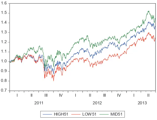
Furthermore an aggregate index (Hindls et al., 2007) was formed for each group. Fig. 2 highlights the development of the aggregated indexes. On average, stocks in the fi rst group (high51) climbed 36%, stocks in the second group (mid51) gained 44% while the third group (low51) grew by 24% during the observed period.

Although the diff erences in the average growth between the individual groups seam considerable at the fi rst sight, disparity of averages was tested. Normality of the data was tested fi rst. Null hypothesis of a normal distribution was rejected by both the Kolmogorov-Smirnov (p-value = 0.000) and Shapiro-Wilk (p-value = 0.000) tests.

1: Long-term development of S & P 500 stock index

Since the null hypothesis of a normal distribution of the data was rejected, a nonparametric test had to be used for testing of disparity of the averages. The nonparametric Kruskal-Wallis test (Hendl, 2009) did not establish disparity of average growth between the groups (p-value = 0.317). Presence of infl uence of the trading volume level of the stocks on their growth was not proved.

Univariate GARCH-class Models

A seminal work of Engle (1982) provided the basis for the family of Autoregressive Conditional Heteroskedasticity (ARCH) models. This group of models is probably still today an unsurpassed tool for volatility modeling. Bollerslev (1986) eliminated some defi ciencies of the original ARCH model by his popular GARCH (generalized ARCH) model.

Cipra (2008) describes the standard GARCH(1,1) model as follows:

yt = μt + et, et = tt, t 2 ₌

= ₀ + ₁e_t2 −1 + 1

2

t−1(0 > 0, 1, 1 ≥ 0, 1 + 1 < 1), (1) where

μt .... denotes the conditional mean and _t2 _{... is the conditional variance.}

Glosten et al. (1993) proposed the GJR model to cope with eff ects of asymmetry. The most used form of the GJR GARCH model is:

y_t = μ_t + e_t, e_t = _t_t, _t2 =  0 + 1e

2 t−1 + 1

2 t−1 + 1et

2 −1I

− t−1, It

− ₌

=  1  if et < 0,

 0 otherwise. (2)

Another approach to asymmetry was shown by Nelson (1991). His exponential GARCH model a er some simplifi cation has the form:

yt = μt + et, et = tt,

 



 

         

 

2 1 2 1

0 1 1 1 1

1 1

ln t ln t

t t

t t

e e

. (3)

GARCH(1,1) is one of the most used models of fi nancial time series because it is capable to handle very general volatility structure using only three parameters (Cipra, 2008).

Next procedures were conducted to construct models with the best possible prediction ability for each aggregated index. As a benchmark an aggregated index of all 475 stocks was analyzed fi rst.

Descriptive Statistics

The time series of the aggregated index of all 475 stocks (all475) shown in Fig. 3 was modifi ed to stationary Log returns (Fig. 4).

The stationarity of the returns was checked by an Augmented Dickey and Fuller unit root test. The optimal lag length of the ADF test was chosen based on Schwarz information criterion (SIC).

Fig. 5 shows residuals calculated as the deviation of the log returns from the mean of the series.

The Jarque and Bera statistic suggested rejection of the null hypothesis of a normal distribution of residuals at the 1% signifi cance level. Tab. I shows that the series has a sharp and negatively skewed distribution. The null hypothesis of autocorrelation in the Breusch and Godfrey Serial Correlation LM Test was not rejected. Presence of autocorrelation was confi rmed also by Ljung and Box Q statistics with the exception of the fi rst lag. In the next step the ARCH LM test was conducted. Since ARCH was 0.7 0.8 0.9 1.0 1.1 1.2 1.3 1.4 1.5 1.6

I II III IV I II III IV I II

2011 2012 2013

HIGH51 LOW51 MID51

2: Development of aggregated indexes

0.8 0.9 1.0 1.1 1.2 1.3 1.4

I II III IV I II III IV I II

2011 2012 2013

3: Aggregated index of all 475 stocks

Source: Bloomberg, EViews, own processing

-8 -6 -4 -2 0 2 4 6

I II III IV I II III IV I II

2011 2012 2013

4: Log returns of aggregated index of all 475 stocks

Source: Bloomberg, EViews, own processing

-8 -4 0 4 8

-8 -4 0 4 8

I II III IV I II III IV I II

2011 2012 2013

Residual Actual Fitted

5: Residuals of the log returns time series

found in the investigated data, this justifi es the use of GARCH models.

The same procedure as for the variable all475 was applied on the other constructed indexes (high51, mid51 and low51). The descriptive statistics and results of the conducted tests are summarized in Tab. I. The results for all the variables are very similar.

RESULTS AND DISCUSSION

From the family of Autoregressive Conditional Heteroskedasticity (ARCH) models (Bollerslev, 1986 and Engle, 1982) three diff erent discussed models were selected for the purpose of capturing the dynamics of volatility.

Tab. II shows the in-sample estimates for GARCH(1,1) model. High values of the estimated

coeffi cients indicate high degrees of volatility persistence. These coeffi cients are all signifi cant at the 1% signifi cance level.

Tab. III presents the results for the GJR model and Tab. IV shows the results for the EGARCH model. For both models the asymmetric coeffi cients are all signifi cant at the 1% signifi cance level.

These results indicate existence of long-memory in the return volatility of the indexes. The numbers in parentheses are the t-statistics of the estimated coeffi cients.

The results of the diagnostic tests are shown in the lower part of the tables. The P-values of the statistics are reported in square brackets. Q(10) and Q(20) are the (Ljung and Box, 1978) Q statistics of order 10 and 20 respectively for the squared standardized residuals. For the series high51, mid51 and low51, Ljung and Box’s Q statistics I: Descriptive statistics and tests

variable all475 high51 mid51 low51

ADF(original) −0.760358 −0.422664 −0.915232 −0.808691 ADF(return) −16.24726 *** −16.37395 *** −16.15876 *** −16.05594 *** mean 0.042617 0.047609 0.056467 0.033476 t-statistic 0.921379 1.130633 1.243562 0.702654 skewness −0.618809 −0.550628 −0.552168 −0.609200 kurtosis 8.330827 7.570283 8.508805 7.964273 Jarque-Bera 809.882 *** 597.6276 *** 853.6104 *** 706.5583 *** Breusch-Godfrey 2.187612 3.047703 1.693607 2.593459 ARCH LM test 42.23387 *** 54.49980 *** 42.62828 *** 45.25625 *** * Denotes rejection of the null hypothesis at 10% signifi cance level.

** Denotes rejection of the null hypothesis at 5% signifi cance level. *** Denotes rejection of the null hypothesis at 1% signifi cance level. Source: Bloomberg, EViews, own processing

II: Estimation results of GARCH(1,1) model

Source: Bloomberg, EViews, own processing

III: Estimation results of GJR model

cannot reject the null hypothesis of no serial correlations at the 10% confi dence level for all models. For the all475 series there is an exception in the GARCH(1,1) model where the null hypothesis is rejected even at the 1% confi dence level for the Q statistics of order 10.

ARCH(10) and ARCH(20) are the ‘non-heteroskedasticity’ statistics (Engle, 1982) of order 10 and 20, respectively. The F-statistics and the related p-values show how well each model captures ARCH eff ects in returns of each time series. Arguably the best results of all the models are provided by EGARCH.

Log(L) is the logarithm maximum likelihood function value. The values of Log(L) are very close to each other across diff erent models but across diff erent time series they have relatively large diff erentials. A similar conclusion was drawn by Wang and Wu (2012) who examined returns in energy markets.

AIC is Akaike information criterion, while BIC is Bayes information criterion which are used as objective criteria and procedures for model selection (Cipra, 2008). In general, according to the information criteria the best results were achieved by the GJR model in all the time series. But the most important result for this investigation is that the lowest values of criteria were achieved for high51 series by each of the three models.

A certain level of trading volume is a generally recognized factor for forming investment strategy.

Rejnuš (2010) states that the level of liquidity together with the rate of profi t and risk infl uence demand for investment instruments. Volume is used also for price movement confi rmation in technical analysis. Volume confi rms power of the prevalent side of market and helps to distinguish diff erent phases of market (accumulation, uptrend, distribution and downtrend) (Turek, 2008).

The results of this paper show that not only the level required to execute a trade can be useful for the investor. The higher the trading volume the better the possibility to predict the development of an investment instrument.

CONCLUSION

The results obtained in this paper are not in confl ict with the initial assumption. The importance of the level of trading volume for the prediction of fi nancial time series development was demonstrated.

As objective criteria for selection of a model with best attributes (i.e. particularly a low number of variables and a low value of residual component variance estimate), Akaike information criterion and Bayes information criterion were used. According to the information criteria the best results were achieved by the GJR model in all the time series. But the most important result is that the lowest values of criteria were achieved for high51 series by each of the three models.

The volatility structure of the examined data supports the idea that infl uential investors respond to various shocks in the market primarily by closing or opening their largest position. This fi nding could help analysts create such volatility structure of time series which would allow them to explain its development by various models with better results.

In light of the achieved results, market participants who use technical analysis should attain the best results of their analysis with application to the most traded stocks. The time series of the price development of these stocks should refl ect new information fastest and most accurately.

In the course of time the process of globalization links fi nancial markets all around the world. The fi nancial time series development depends on an enormous number of independent variables. Some of them are evident but others are unidentifi able. One the one hand, market participants are forced to follow a great number of news but on the other, they are forced to seek the best possibilities of utilizing technical analyses.

A verifi cation of the results and conclusions by application of the used procedure to other time intervals or on other stock indexes would contribute to the examined issue.

IV: Estimation results of EGARCH model

SUMMARY

This article focuses on the infl uence of trading volume on the quality of prediction of stock market development. Most authors examine a dynamic relationship where a time series representing the development of the stock market is the dependent variable and a time series of trading volume is an independent variable entering various models (Chan, 2012; Wang and Huang, 2012; etc.). Compared with this approach, this paper examined if a higher level of trading volume can ensure better results for constructing univariate models.

The research in this paper was applied on the stocks included in the S & P 500 index. From a statistical point of view the longer the series, the better the estimation. On the other hand, the length of the time series had to be limited as the data set contained a great number of series of daily values. As a compromise, given the above limitations, the period from January 2011 to June 2013 was selected. Based on a calculation of average trading volume, three groups of stocks were formed and for each group an aggregate index was constructed. The graphical analyses showed that the stocks with the middle-high trading volume gained 44% on average in the observed period while stocks with the highest volume rose by 36% and those with the lowest volume strengthened only by 24%. However, the Kruskal-Wallis test did not prove presence of infl uence of the trading volume level of the stocks on their growth.

In the next part, The dynamics of index return volatility was modeled by univariate GARCH-class models. GARCH(1,1), GJR and EGARCH models were estimated for each time series. The in-sample evidence indicated that the return volatility of the indexes can be characterized by signifi cant persistence and asymmetric eff ects. In general, according to the information criteria the best results were achieved by the GJR model in all the time series.

Finally, the results of the diagnostic tests on residuals showed that the best estimate of each model was made for the index of stocks with the highest average trading volume.

The results obtained in this paper are not in confl ict with the initial assumption. The importance of the level of trading volume for the prediction of fi nancial time series development was shown.

Acknowledgement

The fi ndings presented in this paper resulted from grant number 20131046 “Vliv objemu obchodů na kvalitu predikce vývoje akciového trhu” (Impact of Trading Volume on Prediction Quality of Stock Market Development) of Internal Grant Agency (IGA) of the Faculty of Economics and Management, Czech University of Life Sciences in Prague.

REFERENCES

ARLT, J., ARLTOVÁ, M. 2009. Ekonomické časové řady.

Praha: Professional Publishing.

BOLLERSLEV, T. 1986. Generalized autoregressive conditional heteroskedasticity. Journal of Econometrics, 31(3): 307–327.

BREMER, C., DMITRACOVA, O. 2011. Analysis: France, Britain AAA-ratings under scrutiny. Reuters (Paris/London), 8 Aug. 2011. [Online]. Available: http://www.reuters.com/article/2011/08/08/ us-crisis-ratings-idUSTRE7773KG20110808. [Accessed: 6 Oct. 2013].

CAMPBELL, J. Y., GROSSMAN, S. J., WANG, J. 1993. Trading volume and serial correlation in stock returns. Quarterly Journal of Economics, 108(4): 905– 939.

CHEN, S. S. 2012. Revisiting the empirical linkages between stock returns and trading volume. Journal of Banking and Finance, 36(6): 1781–1788.

CIPRA, T. 2008. Finanční ekonometrie. Praha: Ekopress. DAN, L., YUAN, Z., ZHONG, W. 2011. The dynamic

relationship among return, volatility and trading volume in China stock market – an empirical study based on quantile regression. In: Proceedings of the Sixth International Symphosium on Corporate Governance, 75–85.

ENGLE, R. F. 1982. Autoregressive conditional heteroskedasticity with estimates of the variance of United Kingdom infl ation.Econometrica, 50(4): 987–1007.

GLOSTEN, L. R. JAGANNATHAN, R., RUNKLE, D. E. 1993. On the relation between the expected value and the volatility of the nominal excess return on stocks.The Journal of Finance, 48(5): 1779– 1801.

HENDL, J. 2009. Přehled statistických metod. Praha: Portál.

HINDLS, R., HRONOVÁ, S., SEGER, J., FISCHER, J. 2007. Statistika pro ekonomy. Praha: Professional Publishing.

KARPOFF, J. M. 1987. The relation between price changes and trading volume: a survey. Journal of Financial and Quantitative Analysis, 22(1): 109–126. KUO, S., HSIAO, J., CHAN, H. 2011. The relationship between stock return volatility and trading volume: evidence from the investors in the Taiwan stock market. In: Environment, Low-Carbon and Strategy.

956–959.

NELSON, D. B. 1991. Conditional heteroskedasticity in asset returns: a new approach. Econometrica,

59(2): 347–370.

PUZZANGHERA, J. 2001. S & P downgrades U.S. credit rating. Los Angeles Times, 6 Aug. 2001. [Online]. Available at: http://articles.latimes. com/2011/aug/06/business/la-fi-us-debt-downgrade-20110806. [Accessed: 6 Oct. 2013]. REJNUŠ, O. 2010. Finanční trhy. Ostrava: KEY

Publishing s. r. o.

TUREK, L. 2008. První kroky na burze. Brno: Computer Press, a. s.

WANG, J. K. 2001. Generation of predictive price and trading volume patterns in a model

of dynamically evolving free market supply and demand. Discrete Dynamics in Nature and Society,

6(1): 37–47.

WANG, T., HUANG, Z. 2012. The relationship between volatility and trading volume in the Chinese stock market: a volatility decomposition perspective. Annals of Economics and Finance, 13(1): 211–236.

WANG, Y. D., WU, C. F. 2012. Forecasting energy market volatility using GARCH models: Can multivariate models beat univariate models?

Energy Economics, 34(6): 2167–2181.