The Effects on Visual Information in a Robot in
Environments with Oriented Contours
Lars Olsson, Chrystopher L. Nehaniv, Daniel Polani
Adaptive Systems Research Group
Department of Computer Science
University of Hertfordshire
College Lane, Hatfield Herts AL10 9AB
United Kingdom
{
L.A.Olsson, C.L.Nehaniv, D.Polani
}
@herts.ac.uk
Abstract
For several decades experiments have been performed where animals have been reared in environments with orientationally restricted contours. The aim has been to flnd out what efiects the visual fleld has on the development of the visual system in the brain. In this paper we describe similar experiments per-formed with a robot acting in an environment with only vertical contours and compare the results with the same robot in an ordinary of-flce environment. Using metric projections of the informational distances between sensors it is shown that all visual sensors in the same vertical column are clustered together in the environment with only vertical contours. We also show how the informational structure of the sensors unfold when the robot moves from the environment with oriented contours to a normal environment.
1.
Introduction
In nature one flnds that most animals are highly adapted to their speciflc environment. One example of this is the wide variety of sensory organs that are well adapted to the speciflc animals and their respec-tive environment (Dusenbery, 1992). It is believed that in many animals the functionality of the sensory organs is almost completely innate while in other an-imals the functionality can be altered by experiences during the lifetime of the speciflc animal. This age-old question of nature versus nurture has been partic-ularly studied in the visual system (Callaway, 1998). Many experiments have been performed with ani-mals where their visual fleld somehow has been re-stricted to contours of a certain orientation, see for example (Wiesel, 1982) and (Callaway, 1998) for an overview. The results of these experiments are not completely conclusive but some experiments show
that animals that have been reared in for example an environment with only vertical contours have more neurons selective for vertical contours. It has also been found that ferrets have more neurons selective for vertical and horizontal contours than other angles (Chapman et al., 1996).
Why is it so that animals have more neurons se-lective for vertical and horizontal contours than con-tours of other angles? In a very interesting study by Coppola et al. (Coppola et al., 1998) the distri-bution of contours of difierent orientations in both man-made environments and a natural forest envi-ronment was analysed. That they found more verti-cal and horizontal contours than oblique angled con-tours in the man-made environments might not be a big surprise. But, interestingly enough, they also found that natural environments contain more ver-tical and horizontal contours than contours of other angles. This might explain why visual systems in-nate have more neurons selective for horizontal and vertical contours.
Why, then, is this important when studying and building robots? In contrast with natural systems, sensors of artiflcial systems are often, due to prac-tical and historical reasons, seen as something that is “given” and flxed. But, given that robots usu-ally are limited by computational resources as well as power consumption, robots need to use their limited resources e–ciently. One way to do this is to try and extract relevant information from the environment as early as possible in the processing steps and then focus the computational resources on these relevant pieces of information. But, how can a robot know what information that is relevant to perform its cer-tain task? One notion of relevant information was introduced and formalized in (Nehaniv, 1999) and extended in (Polani et al., 2001) by associating the relevance of information with the utility to an agent to perform a certain action. Given knowledge of the most relevant information from a number of sensors In Berthouze, L., Kozima, H., Prince, C. G., Sandini, G., Stojanov, G., Metta, G., and Balkenius, C. (Eds.) Proceedings of the Fourth International Workshop on Epigenetic Robotics
it might then be possible to adapt the sensoric sys-tem to discriminate only between events that are of use for the system. The layout of sensors can also be evolved to a certain environment, which for exam-ple has been studied in (Olsson et al., 2004a). It is also possible to use thesensor reconstruction method
flrst described in (Pierce and Kuipers, 1997) and ex-tended in (Olsson et al., 2004b) to flnd sensors that produce the same (redundant) information. If sev-eral sensors produce more or less the same informa-tion the informainforma-tion from all of them but one can be discarded or some of the sensors can be placed at difierent positions.
In this paper we perform a similar experiment sim-ilar to the ones peformed with for example kittens (Wiesel, 1982) with a robot where the robot is acting in an environment with only vertical contours. Us-ing the sensor reconstruction method we show that in this kind of environment most visual sensors produce redundant information and can be discarded without a loss of information. The results also indicate that a rich visual environment is necessary if it is to learn to distinguish between contours of difierent orientation. We also show an example of unfolding of sensors, where the robot moves from the environment with oriented contours to a normal o–ce environment. In this case the sensors move in the metric projections from the clusters of all sensors from a certain column of visual sensors to a layout that re ects the physical layout of the sensors.
The remainder of this paper is organized as fol-lows. Section 2 contains a brief overview of informa-tional distances between sensors and the sensory re-construction method. Section 3 contains the results of the experiments with a robot in an environment with oriented contours, and also results where the robot moves from the vertical environment to a nor-mal environment. Finally we summarize the paper and discuss some potential applications of the results and possible future directions of the presented work.
2.
Information
Distances
between
Sensors
In order to discuss the information distance be-tween sensors a distance metric is needed. To do this a number of difierent methods can used, e.g., the Hamming distance and frequency dis-tribution distance (Pierce and Kuipers, 1997). In (Olsson et al., 2004b) these distance metrics are compared with the information metric, which was deflned and proved to be a metric in (Crutchfleld, 1990). The distance between two infor-mation sources is there deflned in the sense of classi-cal information theory (Shannon, 1948) in terms of conditional entropies. To understand what the infor-mation metric means we need some deflnitions from
information theory.
LetX be the alphabet of values of a discrete ran-dom variable (information source, in this case a sen-sor)X with a probability mass functionp(x), where
x∈ X. Then the entropy, or uncertainty associated withX is
H(X) =¡X
x∈X
p(x) log2p(x) (1)
and the conditional entropy
H(Y|X) =¡X
x∈X
X
y∈Y
p(x, y) log2p(y|x) (2)
is the uncertainty associated with the discrete ran-dom variableY if we know the value of X. In other words, how much more information do we need to fully predictY once we knowX.
Themutual informationis the information shared between the two random variables X and Y and is deflned as
I(X;Y) =H(X)¡H(X|Y) =H(Y)¡H(Y|X). (3)
To measure the dissimilarity of two infor-mation sources Crutchfleld’s inforinfor-mation distance (Crutchfleld, 1990) can be used. The information metric is the sum of two conditional entropies, or formally
d(X, Y) =H(X|Y) +H(Y|X). (4)
Note that X and Y in our system are information sources whose H(Y|X) and H(X|Y) are estimated from the time series of two sensors using (2).
It is worth noting that two sensors do not need to be identical to have a distance of 0.0 using the infor-mation metric. What an inforinfor-mation distance of 0.0 means is that the sensors are completely correlated. As an example, consider two sine-curves where one is the additive inverse of the other. Even though they have difierent values in almost every point the distance is 0.0 since the value of one is completely predictable from the other. In this case, the mutual information, on the other hand, will be equal to the entropy of either one of the sensors.
by considering the time series of sensor values from a particular sensor as an information source X. The distance between two sensors X andY is then computed using equation 4. From this 2-dimensional distance matrix a 2-dimensional metric projection can be created using a number of difierent methods like metric-scaling (Krzanowski, 1988), Sammon mapping, and elastic nets (Goodhill et al., 1995), which positions the sensors in the two dimensions of the metric projection. In our experiments we have used the relaxation algorithm described in (Pierce and Kuipers, 1997).
3.
Experiments and Results
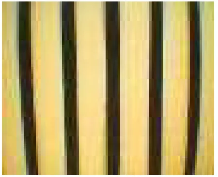
In our experiments we have used a SONY AIBO1 robot dog. The robot walked around more or less at random in an ordinary o–ce environment and one other environment where the visual fleld consists of black vertical lines on a white background. This en-vironment was created with big white sheets of pa-per with 2cm wide stripes of black papa-per glued to the white paper, see Figure 1. Since the AIBO did not move its head up and down and the environment was quite small, most of the collected frames of the visual fleld consisted only of the striped walls but in some frames part of the uniform oor was also visi-ble. Figure 2 shows an example frame captured by the AIBO in the environment with vertical lines.
Figure 1: The SONY AIBO robot in its environment with vertical contours.
To collect data we used the wireless network of the AIBO to download images from the camera of the robot where the image is 88 pixels wide and 72 pixels high. The frame rate was on average 10 frames per second with a minimum of 9.7 frames per second and a maximum of 10.2 frames per second, where the maximum and minimum values were computed
1AIBO is a registered trademark of SONY Corporation.
Figure 2: The environment from the robot’s perspective.
as averages over flve seconds. To make the results of the sensor reconstruction method easier to interpret we used a 10 by 10 pixel image from each frame taken from the upper left corner of the image. The pixels of this 10 by 10 image are numbered from 1 to 100, see Figure 3. To verify that the results were not due to the fact that we only used a part of the visual fleld we performed experiments with the whole image with similar results.
1 2 3 4 5 6 7 8 9 10
11 12 13 14 15 16 17 18 19 20
21 22 23 24 25 26 27 28 29 30
31 32 33 34 35 36 37 38 39 40
41 42 43 44 45 46 47 48 49 50
51 52 53 54 55 56 57 58 59 60
61 62 63 64 65 66 67 68 69 70
71 72 73 74 75 76 77 78 79 80
81 82 83 84 85 86 87 88 89 90
91 92 93 94 95 96 97 98 99 100
Figure 3: The layout of the visual sensors (individual pixels).
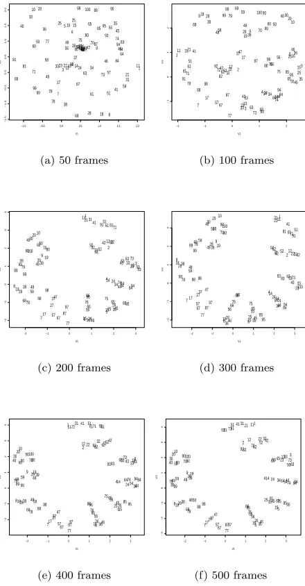
500 frames the sensors are ordered in more or less a square with sensor 1 in the upper right corner and sensor 100 in the lower left corner. Thus, the layout of the sensors shown after 500 frames is the mirror image of the real layout found in Figure 3. This ori-entation of the layout as a mirror image of the real sensors in this case is just a coincidence and in fact all eight possible orientations are equally likely. This is because the data contains no directional informa-tion and it is therefore impossible to flnd the correct physical layout without applying higher-level image analysis. Therefore only the relative positions can be computed, see (Olsson et al., 2004b).
−2 −1 0 1 2
−1 0 1 2 V1 V2 1 2 3 4 5 6 7 8 9 10 11 12 13 14 15 16 17 18 19 20 21 22 23 24 25 26 27 28 29 30 31 32 33 34 35 36 37 38 39 40 41 42 43 44 45 46 47 48 49 50 51 52 53 54 55 56 57 58 5960 61 62 6364 65 66 67 68 69 70 71 72 73 74 75 76 77 78 79 80 81 82 83 84 85 86 87 88 89 90 91 92 93 94 95 96 97 98 99 100
(a) 50 frames
−2 −1 0 1 2
−1 0 1 2 3 V1 V2 1 2 3 4 5 6 7 8 9 10 11 12 13 14 15 16 17 182019
21 22 23 24 25 26 27 28 29 30 31 32 33 34 35 36 37 38 39 40 41 42 43 44 45 46 47 48 49 50 51 52 53 54 55 56 57 58 59 60 61 62 63 64 65 66 67 68 69 70 71 72 73 74 75 76 77 78 79 80 81 82 83 84 85 86 87 88 89 90 91 92 93 94 95 96 97 98 99 100
(b) 100 frames
−3 −2 −1 0 1 2 3
−2 −1 0 1 2 3 4 V1 V2 1 2 3 4 5 6 7 8 9 10 11 12 13 14 15 16 17 18 19 20 21 22 23 24 25 26 27 28 29 30 31 32 33 34 35 36 37 38 39 40 41 42 43 44 45 46 47 48 49 50 51 52 53 54 55 56 57 58 59 60 61 62 63 64 65 66 67 68 69 70 71 72 73 74 75 76 77 78 79 80 81 82 83 84 85 86 87 88 89 90 91 92 93 94 95 96 97 98 99 100
(c) 200 frames
−3 −2 −1 0 1 2 3
−2 −1 0 1 2 3 4 V1 V2 1 2 3 4 5 6 7 8 9 10 11 12 13 14 15 16 17 18 19 20 21 22 23 24 25 26 27 28 29 30 31 32 33 34 35 36 37 38 39 40 41 42 43 44 45 46 47 48 49 50 51 52 53 54 55 56 57 58 59 60 61 62 63 64 65 66 67 68 69 70 71 72 73 74 75 76 77 78 79 80 81 82 83 84 85 86 87 88 89 90 91 92 93 94 95 96 97 98 99 100
(d) 300 frames
−2 0 2 4
−2 −1 0 1 2 3 4 V1 V2 1 2 3 4 5 6 7 8 9 10 11 12 13 14 15 16 17 18 19 20 21 22 23 24 25 26 27 28 29 30 31 32 33 34 35 36 37 38 39 40 41 42 43 44 45 46 47 48 49 50 51 52 53 54 55 56 57 58 59 60 61 62 63 64 65 66 67 68 69 70 71 72 73 74 75 76 77 78 79 80 81 82 83 84 85 86 87 88 89 90 91 92 93 94 95 96 97 98 99 100
(e) 400 frames
−2 0 2 4
−3 −2 −1 0 1 2 3 4 V1 V2 1 2 3 4 5 6 7 8 9 10 11 12 13 14 15 16 17 18 19 20 21 22 23 24 25 26 27 28 29 30 31 32 33 34 35 36 37 38 39 40 41 42 43 44 45 46 47 48 49 50 51 52 53 54 55 56 57 58 59 60 61 62 63 64 65 66 67 68 69 70 71 72 73 74 75 76 77 78 79 80 81 82 83 84 85 86 87 88 89 90 91 92 93 94 95 96 97 98 99 100
(f) 500 frames
Figure 4: Metric projections of the sensors after 50, 100, 200, 300, 400, and 500 frames of visual data in the normal office environment.
Now consider Figure 5 with metric projections for the visual data from the environment with only
ver-tical contours. After 50 frames no real order can be found. After 100 frames it is possible to see that the sensors start to become clustered in a number of groups. After more frames these clusters become
−1.0 −0.5 0.0 0.5 1.0 1.5 2.0
−1.5 −1.0 −0.5 0.0 0.5 1.0 1.5 2.0 V1 V2 1 2 3 4 5 6 7 8 9 10 11 12 13 14 15 16 17 18 19 20 21 22 23 24 25 26 27 28 29 30 31 32 33 34 35 36 37 38 39 40 41 42 43 44 45 46 47 48 49 50 51 52 53 54 55 56 57 58 59 60 61 62 63 64 65 66 67 68 69 70 71 72 73 74 75 76 77 78 79 80 81 82 83 84 85 86 87 88 89 90 91 92 93 94 95 9697 98 99 100
(a) 50 frames
−2 −1 0 1 2
−1 0 1 2 V1 V2 1 2 3 4 5 6 7 8 9 10 11 12 13 14 15 16 17 18 19 20 21 22 23 24 25 26 27 28 29 30 31 32 33 34 35 36 37 38 39 40 41 42 43 44 45 46 47 48 49 50 51 52 53 54 55 56 57 58 59 60 61 62 63 64 65 66 67 68 69 70 71 72 73 74 75 76 77 78 79 80 81 82 83 84 85 86 87 88 89 90 91 92 93 94 95 96 97 98 99 100
(b) 100 frames
−2 −1 0 1 2 3
−2 −1 0 1 2 3 4 V1 V2 1 2 3 4 5 6 7 8 9 10 11 12 13 14 15 16 17 18 19 20 21 22 23 24 25 26 27 28 29 30 31 32 33 34 35 36 37 38 39 40 41 42 43 44 45 46 47 48 49 50 51 52 53 54 55 56 57 58 59 60 61 62 63 64 65 66 67 68 69 70 71 72 73 74 75 76 77 78 79 80 81 82 83 84 85 86 87 88 89 90 91 92 93 94 95 96 97 98 99 100
(c) 200 frames
−2 −1 0 1 2 3
−2 −1 0 1 2 3 V1 V2 1 2 3 4 5 6 7 8 9 10 11 12 13 14 15 16 17 18 19 20 21 22 23 24 25 26 27 28 29 30 31 32 33 34 35 36 37 38 39 40 41 42 43 44 45 46 47 48 49 50 51 52 53 54 55 56 57 58 59 60 61 62 63 64 65 66 67 68 69 70 71 72 73 74 75 76 77 78 79 80 81 82 83 84 85 86 87 88 89 90 91 92 93 94 95 96 97 98 99 100
(d) 300 frames
−2 −1 0 1 2 3
−2 −1 0 1 2 3 4 V1 V2 1 2 3 4 5 6 7 8 9 10 11 12 13 14 15 16 17 18 19 20 21 22 23 24 25 26 27 28 29 30 31 32 33 34 35 36 37 38 39 40 41 42 43 44 45 46 47 48 49 50 51 52 53 54 55 56 57 58 59 60 61 62 63 64 65 66 67 68 69 70 71 72 73 74 75 76 77 78 79 80 81 82 83 84 85 86 87 88 89 90 91 92 93 94 95 96 97 98 99 100
(e) 400 frames
−2 −1 0 1 2 3
−3 −2 −1 0 1 2 3 4 V1 V2 1 2 3 4 5 6 7 8 9 10 11 12 13 14 15 16 17 18 19 20 21 22 23 24 25 26 27 28 29 30 31 32 33 34 35 36 37 38 39 40 41 42 43 44 45 46 47 48 49 50 51 52 53 54 55 56 57 58 59 60 61 62 63 64 65 66 67 68 69 70 71 72 73 74 75 76 77 78 79 80 81 82 83 84 85 86 87 88 89 90 91 92 93 94 95 96 97 98 99 100
(f) 500 frames
Figure 5: Metric projections of the sensors after 50, 100, 200, 300, 400, and 500 frames of visual data in the vertical environment.
from sensors 1,11,21,. . . , 91 we flnd that the next cluster is all sensors in the second column (ending with 2) and so forth. Finally the leftmost cluster of the horse-shoe shape contains all sensors of the right-most column of sensors (10, 20, . . . , 100) in Figure 3.
What is the reason for this clustering of columns of sensors in the vertical environment? In an envi-ronment with only vertical contours and a uniform background all sensors with the same horizontal po-sition will at each time step return the same value. Thus the informational distance between these two sensors will be close to or 0.0. In the results pre-sented in Figure 5 we note that the distance between the sensors in the same column is larger than 0.0. This is due to the fact this is data from the real world and hence the light is difierent in difierent parts of the visual fleld and not all lines are aligned at exactly the same angle. The shape of the group of clusters is dependent on the distribution of vertical lines within the environment and the width of the lines and the robot’s distance to the lines. In this particular ex-periment the vertical lines were often thinner than the width of the visual fleld (10 pixels). Thus we flnd that the informational distance between the two outermost columns is shorter than the distance be-tween for example the leftmost column and the mid-dle columns. This is the reason for the horse-shoe shape of the clusters.
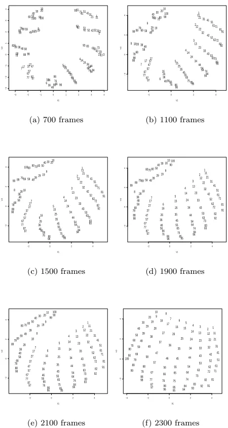
Now consider a situation where the AIBO after 600 time steps move from the environment with only vertical contours to a normal o–ce environment with contours of all angles. In Figure 6 metric projections are shown of the visual sensors after the robot has moved from the vertical environment to the o–ce environment. After 700 time steps the sensors of each vertical column are still clustered together even though they have started to move apart. The longer time that the AIBO has spent in the normal environ-ment the more the metric projection looks like Figure 4 which is the layout of sensors in the normal envi-ronment. This is an example ofunfoldingof sensors where the sensors are separated in the metric pro-jection when they distinguish difierent information.
4.
Conclusions
In this paper we have tried to capture some of the properties of experiments done with real animals in environments with oriented contours in experiments using a real robot. A SONY AIBO robot has moved around in an environment with only vertical con-tours. Metric projections have been created from the visual sensors that show the informational relation-ships between the sensors. The metric projections show that the sensors from the same column in the visual fleld are clustered together which means that
−3 −2 −1 0 1 2 3 4
−3 −2 −1 0 1 2 3 4 V1 V2 1 2 3 4 5 6 7 8 9 10 11 12 13 14 15 16 17 18 19 20 21 22 23 24 25 26 27 28 29 30 31 32 33 34 35 36 37 38 39 40 41 42 43 44 45 46 47 48 49 50 51 52 53 54 55 56 57 58 59 60 61 62 63 64 65 66 67 68 69 70 71 72 73 74 75 76 77 78 79 80 81 82 83 84 85 86 87 88 89 90 91 92 93 94 95 96 97 98 99 100
(a) 700 frames
−2 0 2 4
−2 0 2 4 V1 V2 1 2 3 4 5 6 7 8 9 10 11 12 13 14 15 16 17 18 19 20 21 22 23 24 25 26 27 28 29 30 31 32 33 34 35 36 37 38 39 40 41 42 43 44 45 46 47 48 49 50 51 52 53 54 55 56 57 58 59 60 61 62 63 64 65 66 67 68 69 70 71 72 73 74 75 76 77 78 79 80 81 82 83 84 85 86 87 88 89 90 91 92 93 94 95 96 97 98 99 100
(b) 1100 frames
−2 0 2 4
−2 0 2 4 V1 V2 1 2 3 4 5 6 7 8 9 10 11 12 13 14 15 16 17 18 19 20 21 22 23 24 25 26 27 28 29 30 31 32 33 34 35 36 37 38 39 40 41 42 43 44 45 46 47 48 49 50 51 52 53 54 55 56 57 58 59 60 61 62 63 64 65 66 67 68 69 70 71 72 73 74 75 76 77 78 79 80 81 82 83 84 85 86 87 88 89 90 91 92 93 94 95 96 97 98 99 100
(c) 1500 frames
−2 0 2 4
−2 0 2 4 V1 V2 1 2 3 4 5 6 7 8 9 10 11 12 13 14 15 16 17 18 19 20 21 22 23 24 25 26 27 28 29 30 31 32 33 34 35 36 37 38 39 40 41 42 43 44 45 46 47 48 49 50 51 52 53 54 55 56 57 58 59 60 61 62 63 64 65 66 67 68 69 70 71 72 73 74 75 76 77 78 79 80 81 82 83 84 85 86 87 88 89 90 91 92 93 94 95 96 97 98 99 100
(d) 1900 frames
−2 0 2 4
−2 0 2 4 V1 V2 1 2 3 4 5 6 7 8 9 10 11 12 13 14 15 16 17 18 19 20 21 22 23 24 25 26 27 28 29 30 31 32 33 34 35 36 37 38 39 40 41 42 43 44 45 46 47 48 49 50 51 52 53 54 55 56 57 58 59 60 61 62 63 64 65 66 67 68 69 70 71 72 73 74 75 76 77 78 79 80 81 82 83 84 85 86 87 88 89 90 91 92 93 94 95 96 97 98 99 100
(e) 2100 frames
−4 −2 0 2 4
−2 0 2 4 V1 V2 1 2 3 4 5 6 7 8 9 10 11 12 13 14 15 16 17 18 19 20 21 22 23 24 25 26 27 28 29 30 31 32 33 34 35 36 37 38 39 40 41 42 43 44 45 46 47 48 49 50 51 52 53 54 55 56 57 58 59 60 61 62 63 64 65 66 67 68 69 70 71 72 73 74 75 76 77 78 79 80 81 82 83 84 85 86 87 88 89 90 91 92 93 94 95 96 97 98 99 100
(f) 2300 frames
Figure 6: Metric projections of the sensors after 700, 1100, 1500, 1900, 2100, and 2300 frames of visual data in the normal environment where the robot moved after 600 frames from the vertical environment.
the informational distance between them is small, and would in an simulation without noise be 0.0. We also showed how the sensors unfold in the metric projections when the robot moves from the vertical environment to an o–ce environment with contours of all angles.
robots’ sensors. Consider for example the fact that most mammals have more neurons selective for ver-tical and horizontal contours than contours of other orientations (Callaway, 1998). This can be explained by the fact that most environments contain more contours of those orientations (Coppola et al., 1998). Thus, the mammal visual system has been adapted by flnding generic properties of many difierent en-vironments. Similarly, is it possible to adapt the visual system of robots by studying the properties of the environment that the robot will interact in. This can for example be done using the sensory reconstruction method (Olsson et al., 2004b) or by evolution of the sensory layouts, see for instance (Olsson et al., 2004a). This was illustrated in this paper where the sensors were clustered in ten groups and most of the sensors could have been discarded or moved to other positions on the robot.
There are several issuses that need to be consid-ered when designing a robot with sensors that can adapt and be optimized to a certain environment as discussed above. First of all there is the obvious question of how to actually design a sensoric system that can adapt to a speciflc environment. Another important issuse is how this specialisation might af-fect future adaptations to other environments. For example, consider a robot with a sensoric system op-timized for the environment with only vertical con-tours. How can the robot detect that it has moved to a more complex forrest environment using sensors adapted to the restricted vertical environment? This is related to the trade-ofis between redundancy and novelty that any designer of a sensoric system is faced with (Olsson et al., 2004a). These are all questions that we intend to investigate in future work.
Acknowledgements
We wish to express our gratitude to the anonymous reviewers for their helpful and insightful comments.
References
Callaway, E. M. (1998). Visual scenes and cortical neurons: What you see is what you get. Pro-ceedings of the National Academy of Sciences, 95(7):3344–3345.
Chapman, B., Stryker, M. P., and Bonhoefier, T. (1996). Development of orientation preference maps in ferret primary visual cortex.Journal of Neuroscience, 16(20):6443–6453.
Coppola, D., Purves, H. R., McCoy, A. N., and D., P. (1998). The distribution of oriented contours in the real world. InProceedings of the National Academy of Sciences, volume 95, pages 4002– 4006.
Crutchfleld, J. P. (1990). Information and its Met-ric. In Lam, L. and Morris, H. C., (Eds.), Non-linear Structures in Physical Systems – Pattern Formation, Chaos and Waves, pages 119–130. Springer Verlag.
Dusenbery, D. B. (1992). Sensory Ecology. WH Friedman & Co, flrst edition.
Goodhill, G., Finch, S., and Sejnowski, T. (1995). Quantifying neighbourhood preservation in to-pographic mappings. Institute for Neural Com-putation Technical Report Series, No. INC-9505.
Krzanowski, W. J. (1988). Principles of Multivari-ate Analysis: A User’s Perspective. Clarendon Press, Oxford.
Nehaniv, C. L. (1999). Meaning for observers and agents. In IEEE International Symposium on Intelligent Control / Intelligent Systems and Semiotics, ISIC/ISIS’99, pages 435–440. IEEE Press.
Olsson, L., Nehaniv, C. L., and Polani, D. (in press, 2004a). Information trade-ofis and the evolution of sensory layouts. InNinth International Con-ference on the Simulation and Synthesis of Liv-ing Systems (ALIFE9) September 12-15th 2004 Boston, Massachusetts, USA. MIT Press.
Olsson, L., Nehaniv, C. L., and Polani, D. (in press, 2004b). Sensory channel grouping and struc-ture from uninterpreted sensor data. In 2004 NASA/DoD Conference on Evolvable Hardware June 24-26, 2004 Seattle, Washington, USA. IEEE Computer Society Press.
Pierce, D. and Kuipers, B. (1997). Map learning with uninterpreted sensors and efiectors. Artifl-cial Intelligence, 92:169–229.
Polani, D., Martinetz, T., and Kim, J. (2001). An information-theoretic approach for the quantifl-cation of relevance. In Kelemen, J. and Sos´ık, P., (Eds.), Advances in Artiflcial Life, 6th Eu-ropean Conference, ECAL 2001, Prague, Czech Republic, September 10-14, 2001, Proceedings, Lecture Notes in Computer Science, pages 704– 713. Springer Verlag.
Shannon, C. E. (1948). A mathematical theory of communication. Bell System Tech. J., 27:379– 423, 623–656.
Wiesel, T. (1982). Postnatal development of the visual cortex and the in uence of environment.