www.nonlin-processes-geophys.net/15/987/2008/ © Author(s) 2008. This work is distributed under the Creative Commons Attribution 3.0 License.
Nonlinear Processes
in Geophysics
Comparative rainfall data analysis from two vertically pointing
radars, an optical disdrometer, and a rain gauge
E. I. Nikolopoulos1,*, A. Kruger1,2, W. F. Krajewski1, C. R. Williams2, and K. S. Gage2
1IIHR-Hydroscience & Engineering, University of Iowa, Iowa City, Iowa, USA
2Cooperative Institute for Research in Environmental Sciences, University of Colorado and Physical Sciences Division,
NOAA Earth System Research Laboratory, Boulder, Colorado, USA
*currently at: University of Connecticut, Storrs, USA
Received: 17 July 2007 – Revised: 31 October 2008 – Accepted: 6 November 2008 – Published: 16 December 2008
Abstract. The authors present results of a comparative
anal-ysis of rainfall data from several ground-based instruments. The instruments include two vertically pointing Doppler radars, S-band and X-band, an optical disdrometer, and a tipping-bucket rain gauge. All instruments were collocated at the Iowa City Municipal Airport in Iowa City, Iowa, for a period of several months. The authors used the rainfall data derived from the four instruments to first study the temporal variability and scaling characteristics of rainfall and subse-quently assess the instrumental effects on these derived prop-erties. The results revealed obvious correspondence between the ground and remote sensors, which indicates the signifi-cance of the instrumental effect on the derived properties.
1 Introduction
Theoretical and practical needs in hydrology and other geo-sciences stimulated much interest in research of rainfall fun-damental properties. Problems of rainfall estimation using remote sensing and prediction at a wide range of temporal and spatial scales motivate efforts to improve our understand-ing of rainfall variability and dynamics. High resolution and quality observations are required for the task. Although most of our knowledge about rainfall comes from operational net-works of rain gauges and weather radars, specialized instru-ments play increasing important role in filling resolution gaps (Krajewski and Smith, 2002; Krajewski et al., 2006).
In this paper we discuss results of rainfall characteriza-tion using four different collocated instruments that include a tipping-bucket rain gauge, a Parsivel optical disdrometer, and S-band and X-band vertically pointing Doppler radars (profilers). This physical setup of collocated instruments and
Correspondence to: A. Kruger ([email protected])
the fact that the profilers measure radar reflectivity essen-tially continuously in time and with high spatial resolution close to the ground represents the most favorable scenario for the intercomparison of the instruments. Thus, our em-phasis is on addressing the issue of instrumental effects on the analyses rather than the methods themselves. Our char-acterization of variability includes autocorrelation, spectral, and moment scaling analyses in time from the recorded time series of data. Comparison of the results between the instru-ments allows exploring the instrumental-dependence of the derived rainfall properties.
We organized this paper as follows. In Sect. 2 we de-scribe the experimental setup and some technical character-istics and the sampling strategies of the instruments we used in this study. In Sect. 3 we elaborate on the preparation of our data sets. Considerable data processing was required be-fore we could begin our comparative analysis. In Sect. 4 we present the results of the different analysis we performed and in Sect. 5 we summarize and discuss the basic implications of our results.
2 Experimental setup and instrumentation
We operated two in-situ devices, i.e. a double tipping-bucket rain gauge and a Parsivel optical disdrometer and two re-mote sensors, i.e. an S-band and an X-band vertically point-ing radar. The two VPRs and the Parsivel disdrometer were collocated within a 20 m radius (Fig. 1). The dual tipping-bucket rain gauge platform was located some 200 m away from the rest of the equipment.
988 Figures E. I. Nikolopoulos et al.: Scaling analysis of rain data from collocated instruments
4 km
±
4 km±
Fig. 1. Annotated aerial photograph of the Iowa City Municipal Airport. The yellow grid corresponds to the NEXRAD scanning radar grid, the yellow circles represent the VPR's beam area, and the red dots represent the rain gauges. The inset is an aerial photograph of the experimental site at the Iowa City Municipal Airport.
Fig. 1. Annotated aerial photograph of the Iowa City Municipal Airport. The yellow grid corresponds to the NEXRAD scanning radar grid, the yellow circles represent the VPR’s beam area, and the red dots represent the rain gauges. The inset is an aerial photograph of the experimental site at the Iowa City Municipal Airport.
of Level II reflectivity data of the NEXRAD’s WSR-88D weather radar located in Davenport, Iowa, i.e. some 80 km east of the Iowa City Municipal Airport. Note the differ-ences in scales when comparing observations from different sensors.
Each of the instruments considered has unique advantages and limitations. Rain gauges are relatively inexpensive, reli-able instruments, and the uncertainties associated with their observations are fairly well recognized (Habib et al., 1999, 2001; Ciach, 2003; Sieck et al., 2007). However, due to their point-like sampling area, the degree to which they represent larger spatial scales depends on the temporal scale of integra-tion and remains an important subject of hydrologic studies (e.g. Bras and Rodriguez-Iturbe, 1985; Kitchen and Blackall, 1992; Krajewski et al., 2003; Ciach and Krajewski, 2006). Disdrometers share the same limitations as rain gauges but due to their ability to measure individual drops provide use-ful information about rain structure that cannot be obtained from rain gauges. The unit we used and its evaluation is dis-cussed in detail by Krajewski et al. (2006).
Vertically pointing Doppler radars provide valuable in-formation about precipitation structure and characterization (e.g. Atlas et al., 1973; Hauser and Amayenc, 1983; Williams et al., 1995). We operated an S-band (2.835 MHz) VPR (Fig. 1) that belongs to the NOAA Aeronomy Laboratory (Williams et al., 2005). The NOAA S-band samples the atmospheric profile with a spatial resolution of 60 m with the first range gate at 170 m above ground level. It has a parabolic dish diameter of 3.048 m and a beam width of 2.5◦ that results in a sampling bin with a volume at the order of 340×103m3and a diameter of 44 m at 1 km height.
The second profiler that we operated is an X-band (9.410 MHz) vertically pointing Doppler radar that it is
20 30 40
1 2 3 4 5
Reflectivity (dBZ)
H
e
ig
ht
a
b
o
v
e t
h
e gr
o
u
n
d
(
k
m
) 4392 m
2292 m
492 m a)
0 10 20 30 40 50 60 20
25 30 35 40 45
Time (min)
d) 492 m
20 25 30 35 40 45
c) 2292 m
20 25 30 35 40 45
b) 4392 m dBZ
20 30 40
1 2 3 4 5
Reflectivity (dBZ)
H
e
ig
ht
a
b
o
v
e t
h
e gr
o
u
n
d
(
k
m
) 4392 m
2292 m
492 m a)
0 10 20 30 40 50 60 20
25 30 35 40 45
Time (min)
d) 492 m
20 25 30 35 40 45
c) 2292 m
20 25 30 35 40 45
b) 4392 m dBZ
Fig. 2. Time series extracted from S-band profiler’s data. Mean vertical profile of reflectivity (a), based on the storm events during May 25 (black) and June 04 (grey), 2002.. The horizontal thick lines correspond to the three heights from which we extracted our time series. Time series of reflectivity (b), (c), and (d) correspond to heights 4392, 2292, and 492 m above the ground, respectively. The time series data are part of the storm event during May 25, 2002 and are shown for both S-band (black) and X-band (grey).
Fig. 2. Time series extracted from S-band profiler’s data. Mean vertical profile of reflectivity (a), based on the storm events during 25 May (black) and 04 June (grey) 2002. The horizontal thick lines correspond to the three heights from which we extracted our time series. Time series of reflectivity (b), (c), and (d) correspond to heights 4392, 2292, and 492 m above the ground, respectively. The time series data are part of the storm event during 25 May 2002 and are shown for both S-band (black) and X-band (grey).
housed at the IIHR’s Mobile Rainfall Observatory trailer (Fig. 1). The X-band’s spatial resolution is 150 m and the lowest gate is located at 150 m above ground level. It has a parabolic dish diameter of 1.2 m protected and a beam width of 1.9◦ that results in a sampling bin with a volume at the order of 439×103m3and a diameter of 33 m at 1 km height.
3 Data preparation
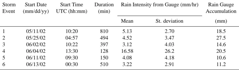
The dataset covers a period of 47 consecutive days beginning 11 May 2002 and ending 26 June 2002. While both VPRs operated most of the time, some gaps in the data record oc-curred because of computer and/or power failure. Compari-son with the rain gauge data from the Iowa City Municipal Airport rain gauge network revealed that most of the missing data corresponded to no rain data. For our analysis, we either used the entire data set or focused on a number of selected storms (Table 1). For the analysis, we extracted time series (from the S-band profiler data) at three heights: close to the ground (492 m), close to but below the bright band (2292 m), and close to but above the bright band (4392 m) (Fig. 2).
Table 1. Selected storm events.
Storm Start Date Start Time Duration Rain Intensity from Gauge (mm/hr) Rain Gauge
Event (mm/dd/yy) UTC (hh:mm) (min) Accumulation
Mean St. deviation (mm)
1 05/11/02 10:20 810 5.13 2.70 18.5
2 05/25/02 04:57 494 4.52 3.47 27.5
3 06/02/02 10:22 397 3.12 4.03 14.6
4 06/04/02 13:30 128 16.58 26.2 20.5
5 06/11/02 09:30 150 4.08 4.18 10.6
6 06/13/02 00:30 510 3.22 2.91 11.2
Nikolopoulos (2004). In the following section we focus mainly on the profilers and we discuss some key issues that one should consider when comparing observations from dif-ferent VPRs.
3.1 Temporal and spatial scale matching
The two radars have different sampling schemes and differ-ent temporal and spatial resolutions. Surprisingly, since the two instruments are collocated, these differences can have profound effect on a comparative analysis. For meaningful comparison, one has to average/combine and resample the data to get the time and spatial scales consistent.
As mentioned before, the S-band samples the vertical pro-file of the atmosphere with a spatial resolution of 60 m, whereas the X-band has a spatial resolution of 150 m. To make comparable spatial bins, we combined S-band radar bins to match the size of the X-band radar bins as closely as possible. More specifically, we combined two S-band bins to get a bin size of 120 m in order to compare with the 150 m bin size of the X-band. When combining the two bins,Xand
Y, one should remember that what the radar would measure if the actual bin size wasX+Y, is not the simple arithmetic average of the measured variables from bin X and bin Y. LetZi(mm6m−3)be the reflectivity factor, measured by the
radar in bini. When we combine the two bins,XandY, the resulting binQ=X+Y will have
ZQ=
Dmax
X
D=0
n
X(D)+nY(D)
volume of binQ
D61D (1)
wherenx(D)andny(D)is the number of drops (of diameter
D) in binXandY respectively. Dmaxis the maximum drop
diameter and1Ddefines the differential drop diameter. In our analysis we assumed that the two consecutive bins (XandY) have equal volumes so we simplified Eq. (1) to
ZQ=
Dmax
X
D=0
n
X(D)
2×volume of binX +
nY(D)
2×volume of binY
D61D= ZX+ZY
2 (2)
Despite the matching of the sampling volumes in the vertical direction, there is still significant difference between the two volumes due to the difference in the beamwidth. The com-bined S-band bins compared with the X-band bin result in a volume difference of the order of 241×103m3at a height of 1 km, which is equivalent to about 55% percent of the X-band bin volume at this height.
We try to mimic the S-band’s sampling strategy by time averaging the X-band’s samples. S-band samples continu-ously for about 8 s, takes 1 s to write the data in the computer disc, and produces 9 s samples, whereas the X-band produces samples every 0.25 s. In order to eliminate this sampling scheme effect, we need to combine 32 of the X-band sam-ples (32 samsam-ples×0.25 s/sample=8 s) using the same averag-ing methodology that we described above to reproduce what the X-band would measure if it was sampling continuously for 8 s. Basically, we are averaging in time by weighting again with the number of hydrometeors per sample. To ac-count for the S-band’s “dead time” of 1 s, every time that we average 32 X-band samples we skip 4 samples (equal to 1 s), and then we repeat the procedure.
3.2 Radar calibration
Both radars were calibrated to account for and minimize the systematic errors in our profiler observations. Clark et al. (2003) and Williams et al. (2003) used observations from a Joss-Waldvogel disdrometer to calibrate vertically pointing radar. We followed a similar technique but used observations from the collocated Parsivel disdrometer. The great advan-tage of using a disdrometer is that in a sense it extends the measurement of reflectivity factor to the surface (Clark et al., 2003), which allows the comparison with the profiler to be made directly on reflectivity space.
3.3 Optimal comparison time scale
990 E. I. Nikolopoulos et al.: Scaling analysis of rain data from collocated instruments
20 30 40
S
-b
a
n
d
R
e
fl
e
c
ti
v
it
y
(d
B
Z
)
a) Before Calibration b) After Calibration
20 30 40
Parsivel Reflectivity (dBZ)
d) After Calibration
20 30 40
20 30 40
X
-b
a
n
d
R
e
fl
e
c
ti
v
ity
(d
B
Z
)
Parsivel Reflectivity (dBZ)
c) Before Calibration 20
30 40
S
-b
a
n
d
R
e
fl
e
c
ti
v
it
y
(d
B
Z
)
a) Before Calibration b) After Calibration
20 30 40
Parsivel Reflectivity (dBZ)
d) After Calibration
20 30 40
20 30 40
X
-b
a
n
d
R
e
fl
e
c
ti
v
ity
(d
B
Z
)
Parsivel Reflectivity (dBZ)
c) Before Calibration
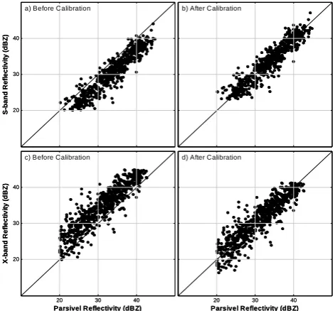
Fig. 3. Comparison between profiler (S-band and X-band) and Parsivel disdrometer reflectivity (dBZ) observations before calibration (a, c) and after calibration (b, d). Fig. 3. Comparison between profiler (S-band and X-band) and
Par-sivel disdrometer reflectivity (dBZ) observations before calibration (a, c) and after calibration (b, d).
profiler is averaged over a significantly larger volume than that of the disdrometer (some nine orders of magnitude), it requires the disdrometer observations to be averaged over a time scale (1T) to best represent the volume-averaged re-flectivity by the profiler. The second issue concerns the fact that the volume observed by the profiler at a certain height will take some time to reach the disdrometer at the ground. This time offset (τ) is related to the height of the observa-tion and the falling speed of the drops inside the volume. Habib and Krajewski (2002) investigated these issues, but they compared radar-rainfall products with a resolution of 2×2 km with rain gauge observations. We largely followed their methodology by using correlation-based analysis to de-termine the optimal comparison time scale.
After the time scale matching between the profilers, we had reflectivity samples every 9 s while the disdrometer pro-duces 30 s samples. We chose the closest to the ground use-able range-gate from the profiler to compare with the dis-drometer. For the S-band, the first available gate is at 185 m, and for the X-band, it is at 492 m. The lower gates for the X-band were contaminated with high signal noise, thus were not available for this analysis. We compared the observations from the profilers at these heights with the disdrometer ob-servations shifted byτ and averaged over1T with a range forτ between−30 and 30 min and for1T between 1.5 and 30 min. We optimized the correlation between the compared reflectivity values to determine the optimalτ and1T.
Optimal time shifts were found around 1.5–3 min, which can be explained if you consider that an average drop (1 mm diameter) with a fall speed of approximately 4 m s−1 takes
about 2 min to reach the ground from a height of 492 m. The highest correlation was obtained for1T around 1.5–5 min. Habib and Krajewski (2002) showed an optimal range forτ
values between 2–5 min and for1T values between 5 and 15 min. The differences in our results are due to the fact that their radar observations were related to higher altitudes (requiring more time to reach the ground) and larger volumes (requiring larger integration scales) than our observations. 3.3.1 Calibration scheme and results
We calibrated the two radars after determining the optimal comparison time scale between the disdrometer and the pro-filers. As above, we extracted the data from the gates clos-est to the ground and compared them with the disdrometer observations. We compared the reflectivity values in dBZ, and the calibration model we applied had the following form (Clark et al., 2003)
ZCAL=ZRAW+C (3)
where ZCAL (dBZ) is the profiler calibrated reflectivity,
ZRAW (dBZ) is the reflectivity measured by the profiler, and
C (dB) is the calibration constant. When we calibrate, we simply want to adjust our values so that the mean difference between the reflectivity values from the disdrometer and the profiler goes to zero. Based on this, we obtained the calibra-tion constant using the following formula
C=E{ZD−ZRAW} (4)
whereEis the expectation operator andZD(dBZ) is the
re-flectivity value we obtained from the disdrometer data when we shifted them byτ and averaged them over1T.
For the calibration procedure, we used data values above 20 dBZ to avoid noisy data that were not removed by the fil-tering techniques and set an upper threshold at 45 dBZ be-cause of the limited sample size of values above this limit. We divided the data in 5 dB bins and classified all the values that were higher than three standard deviations within the bin as outliers and removed them from the data.
The results from the calibration procedure revealed that the S-band observations were underestimated (Fig. 3a) with a mean difference between the reflectivity values from the dis-drometer equal to 3 dB and a standard deviation of 2 dB while the X-band’s were overestimated (Fig. 3c) with a mean equal to 3.6 dB and a standard deviation 2.5 dB. The distributions of differences between the profilers (S-band and X-band) and Parsivel (not shown here) have a similar normal-like shape, with that of the S-band being a little bit narrower due to the 0.5 dB difference of the standard deviations.
4 Analysis of rainfall characteristics
height of 492 m and converted them to rain rate using the well known Z-R relationship of Marshall and Palmer (1948). In some cases we examined the 47 days dataset as one time series and in other cases we performed a storm-based anal-ysis. We attempted to classify the storm events that passed overhead using the high-resolution data collected from the S-band VPR. This gave our analysis a further advantage be-cause we were able to link certain rainfall characteristics with the type of rainfall. We generally followed the classification algorithm described by Williams et al. (1995), but whereas they used a 915 MHz profiler for classification of precipitat-ing clouds in the tropics, we used a 2835 MHz profiler at a mid-western precipitation regime. Thus, in order to evaluate the effectiveness of the algorithm, we recalibrated the pa-rameters and we used manually classified cases to compare against the algorithm’s results.
4.1 Autocorrelation analysis
We performed a storm-based analysis to investigate the be-havior of autocorrelation and the differences between the in-struments for different rainfall events. We analyzed all the storm events described in Table 1. For the autocorrelation calculations, we used 4.5 min averaged rain rates from all instruments. We chose this as an optimal comparison time scale to minimize the effect of local random errors in rain gauge data and to keep the temporal resolution as high as possible. In the calculations we made an assumption of sta-tistical stationarity of the rainfall process within each storm. While the validity of this assumption could be disputed, our focus is on the inter comparison of the instruments. Station-arity assumption is unlikely to affect our conclusions regard-ing ability of different instruments to characterize rainfall.
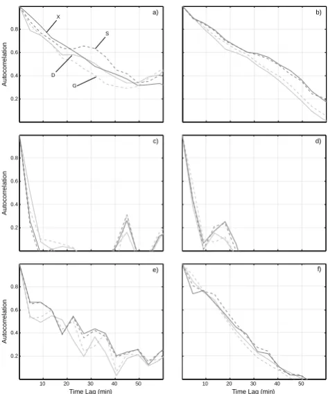
In Fig. 4, we present the results from the autocorrelation calculations from the four instruments and for the six storm events. Generally, there is very good agreement among the four instruments. The most prominent feature is the differ-ence in autocorrelation for different storms. The time re-quired for the autocorrelation to reach a minimum signifi-cant correlation value (1/e) varies from 5 min (Fig. 4d) to 40 min (Fig. 4b). Based on our precipitation classification results, the storms with fast decay of autocorrelation are as-sociated with convective precipitation. This was expected, as the convective precipitation regimes are characterized by high temporal variability. On the contrary, stratiform type of precipitation is more homogeneous and is associated with slow decay of autocorrelation. The differences between the instruments do not appear to have a clear relationship with the precipitation type. Another noticeable feature is that, in most cases, the autocorrelation from the VPR is higher than the one from the rain gauge and disdrometer. This effect is related to the differences in sampling volume. The pro-filer’s observations are averaged over a much larger volume, which results in an increase in the correlation. Instead of a smooth continuous decrease of the correlation with time, in
b)
d) 0.2
0.4 0.6 0.8
A
u
to
c
o
rre
la
ti
o
n
a) X
S
D
G
0.2 0.4 0.6 0.8
A
u
to
c
o
rre
la
ti
o
n
c)
10 20 30 40 50 Time Lag (min)
f)
10 20 30 40 50 0.2
0.4 0.6 0.8
Time Lag (min)
A
u
to
c
o
rr
el
at
io
n
e)
b)
d) 0.2
0.4 0.6 0.8
A
u
to
c
o
rre
la
ti
o
n
a) X
S
D
G
0.2 0.4 0.6 0.8
A
u
to
c
o
rre
la
ti
o
n
c)
10 20 30 40 50 Time Lag (min)
f)
10 20 30 40 50 0.2
0.4 0.6 0.8
Time Lag (min)
A
u
to
c
o
rr
el
at
io
n
e)
Fig. 4. Autocorrelation based on 4.5 min averaged rain rate observations from rain gauge (G), Parsivel disdrometer (D), S-band VPR (S), and X-band VPR (X). The six storm events we analyzed include May 11 (a), May 25 (b), June 02 (c), June 04 (d), June 11 (e), and June 13 (f), 2002.
Fig. 4. Autocorrelation based on 4.5 min averaged rain rate obser-vations from rain gauge (G), Parsivel disdrometer (D), S-band VPR (S), and X-band VPR (X). The six storm events we analyzed include 11 May (a), 25 May (b), 2 June (c), 4 June (d), 11 June (e), and 13 June (f), 2002.
some cases we observe consecutive increases and decreases of the autocorrelation (Fig. 4e), which are mainly associated with oscillations in the rainfall time series.
992 E. I. Nikolopoulos et al.: Scaling analysis of rain data from collocated instruments 0.2 0.4 0.6 0.8 A u to c o rr el at io n 4392 m a) 0.2 0.4 0.6 0.8 A u to c o rr el at io n 2292 m c)
10 20 30 40 50 0.2
0.4 0.6 0.8
Time Lag (min)
A u to c o rre la ti o n 492 m e) 4392 m b) 2292 m d)
10 20 30 40 50
Time Lag (min)
492 m f) 0.2 0.4 0.6 0.8 A u to c o rre la ti o n 4392 m a) 0.2 0.4 0.6 0.8 A u to c o rr el at io n 2292 m c)
10 20 30 40 50 0.2
0.4 0.6 0.8
Time Lag (min)
A u to c o rre la ti o n 492 m e) 4392 m b) 2292 m d)
10 20 30 40 50
Time Lag (min)
492 m f)
Fig. 5. Autocorrelation of rain rate time series derived from S-band (grey) and X-band (black) 9 s resolution data for three different heights and for two different events. The stratiform event (a), (c), (e) during May 25, 2002 and the convective event (b), (d), (f) during June 04, 2002.
Fig. 5. Autocorrelation of rain rate time series derived from S-band (grey) and X-S-band (black) 9 s resolution data for three different heights and for two different events. The stratiform event (a), (c), (e) during 25 May 2002 and the convective event (b), (d), (f) during 4 June 2002.
Z-R revealed no significant difference that would alter our conclusions.
Note that Figs. 4b and 5e correspond to the same event but there is a small difference in autocorrelation from the two profilers. The reason is that in the case of Figure 4b we used rain rates averaged over 4.5 min, which resulted in higher correlation values compared to that of Fig. 5e which was based on 9 s rain rates.
4.2 Spectral analysis
We also performed spectral analysis on our precipitation sig-nal to investigate the variability of precipitation as a function of scale. Following a methodology similar to Fabry (1996), we calculated the power spectrum of our rain rate time se-ries retrieved from both profilers. We performed the power spectrum calculations on a daily basis for the two selected events. A daily precipitation signal consists of 9600 sample points (1 sample per 9 s). To compute the power spectra of this signal we used a length of Fast Fourier Transformation points equal to 1024 and applied a Hanning window with a 50% overlap. In Fig. 6, we present the results obtained for the different heights and different storm events.
The power spectra of a signal are related to its scaling properties. For multiscaling or multiaffine fields, the Fourier
10-4 10-3 10-2 10-1
Frequency (relative units) •← 1 minute
•← 1 hour •← 1 minute
•← 1 hour β1=1.36
β1=1.42
β2=3.34
β2=2.91 492 m f) β=1.83 β=1.67 2292 m d) β=2.28 β=1.94
b) 4392 m
10-4 10-3 10-2 10-1
10-6 10-4 10-2 100 102 104
Frequency (relative units)
P o w e r (re la ti v e u n it s )
•← 1 minute •← 1 hour
492 m β=1.76 β=1.87 e) 10-6 10-4 10-2 100 102 104 P o w e r (re la ti v e u n it s ) β=1.57 β=1.69 2292 m c) 10-6 10-4 10-2 100 102 104 P o w e r (re la ti v e u n it s ) β=1.82 β=1.94 4392 m a) S-band X-band
10-4 10-3 10-2 10-1
Frequency (relative units) •← 1 minute
•← 1 hour •← 1 minute
•← 1 hour β1=1.36
β1=1.42
β2=3.34
β2=2.91 492 m f) β=1.83 β=1.67 2292 m d) β=2.28 β=1.94
b) 4392 m
10-4 10-3 10-2 10-1
10-6 10-4 10-2 100 102 104
Frequency (relative units)
P o w e r (re la ti v e u n it s )
•← 1 minute •← 1 hour
492 m β=1.76 β=1.87 e) 10-6 10-4 10-2 100 102 104 P o w e r (re la ti v e u n it s ) β=1.57 β=1.69 2292 m c) 10-6 10-4 10-2 100 102 104 P o w e r (re la ti v e u n it s ) β=1.82 β=1.94 4392 m a) S-band X-band
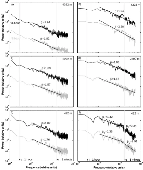
Fig. 6. Power spectra of precipitation rates as derived by the S-band (grey) and X-band (black) VPR at three different heights for two different storms. The stratiform event (a), (c), (e), during May 25, 2002 and the convective (b), (d), (f) during June 04, 2002. Note that we shifted (multiplied by a factor of 102
) the X-band spectra for better display.
Fig. 6. Power spectra of precipitation rates as derived by the S-band (grey) and X-band (black) VPR at three different heights for two different storms. The stratiform event (a), (c), (e), during 25 May 2002 and the convective (b), (d), (f) during 4 June 2002. Note that we shifted (multiplied by a factor of 102)the X-band spectra for better display.
power spectrum exhibits a power law behavior of the form
P ∼f−β (5)
whereP is the power in relative units, f is the frequency in relative units, andβ is the power law exponent usually determined by the slope of the spectrum on a log-log plot (Harris et al., 1998). One basic assumption that we imply in order to perform the spectral analysis is that our signal is stationary. Otherwise, the Fourier power spectrum is not defined. The spectra we obtained from both radars are in good agreement for all the heights and both storm events. We estimated the exponentβ based on least squares linear regression, and the results revealed that the X-band data were consistently associated with higher values, except in the case of 4392 m height for the convective storm.
for the 492 m and used the whole spectra to fit the lines for the heights of 2292 and 4392 m.
The stratiform event we examined revealed a break in the power law behavior at scales around 30 s that was fol-lowed by a flattening of the power spectra. This indicates a near white-noise variability at smaller time scales. Sim-ilar behavior of the spectra is not apparent in Georgakakos et al. (1994), but Fabry (1996) obtained similar results with the main difference being that he observed the break in the slope at smaller time scales (around 5 s). This flat regime of the spectra is translated as a lack of precipitation structure at these small time scales. Fabry (1996) suggested that the spreading of hydrometeors when submitted to wind shear, because of their differential fall speeds, will result in an in-creasing loss of precipitation structure with distance below the generating point of hydrometeors, which can explain the nearly white-noise variability at small scales. The break be-tween the power law and the almost flat spectrum occurs at larger scales above the melting layer (Fig. 6a) than below it (Fig. 6c), which indicates, as Fabry (1996) suggested, that the melting layer reintroduces small-scale structure into the precipitation field.
In the convective case, we did not observe a similar regime of near flat spectra, which indicates that convective precipi-tation exhibits structure at smaller scales than stratiform. In addition, the fact that precipitation structure varies with pre-cipitation type reinforces the likelihood that the observed flat spectra regime for the stratiform case is not an artifact of the instrument. The most prominent feature in the convective case is that the spectra from precipitation signal close to the ground (Fig. 6f) reveal a break in the slope at a time scale close to 1.5 min. The spectral regime at time scales smaller than the break point is characterized by a much steeper slope (approximately equal to 3) than that for larger time scales (approximately equal to 1.5). These two different regimes suggest that two different scaling regimes govern our rain-fall signal. The reason that this break does not appear in the higher altitudes is unclear.
The results from our spectral exponent estimation for time scales larger than 1 min, for the heights of 492 and 2292 m and for both events, vary between 1.36 and 1.87 and are in general agreement with the one obtained by Georgakakos et al. (1994). These exponents are close to the classical Kol-mogorov f−1.66 power law relationship, which represents the spectrum predicted for the fluctuations of a passive scalar introduced into a turbulent fluid (Olsson et al., 1993). The latter suggests that precipitation structure at these scales is turbulence driven.
4.3 Moment scaling analysis
Scaling properties of rainfall in spatial and temporal domain is a topic of growing interest in the last decades. Researchers have used a variety of approaches to investigate the scaling properties of the rainfall process, with multifractal analysis
being the most popular (Olsson et al., 1993; Harris et al., 1997, 1998; de Lima and Grasman, 1999; Kiely and Ivanova, 1999). Following the same spirit with previously we try to in-vestigate the instrumental effect on the derived scaling prop-erties of rainfall by comparing the results we obtained from the four instruments.
The concept of temporal scale invariance (scaling) holds for the rainfall field when the momentMq of orderq≥0 of
the field at a temporal scale,t, is related to the same moment
Mqat a different scaleλtaccording to the relationship
Mq(λt )=λK(q)Mq(t ) (6)
whereK(q)is the scaling exponent or the so-called moment scaling function andλis the scaling factor that we define as the ratio of the given scaletj and a reference scalet0,
λ= tj
t0
(7) Based on the above,λis always≥1. The moment of order q of a discrete random variableXis defined as
Mq =
X
allxi
(xi)qpX(xi) (8)
wherexiis the value ofXat pointiandpXis the probability
mass function ofX(Kottegoda and Rosso, 1997). Based on Eq. (8), we calculated the moments of orderq(0≤q≤5) start-ing at the finest resolution of our data and then degraded the resolution by averaging and recalculated the moments. By repeating this process for different resolutions, we calculated
Mqfor a range of different scales. In order to obtain the value
ofK(q), we plotted the values of logMq against the log of
scaling factor, logλ, and fitted a line based on least squares regression to determine the slope of the line. The value of the slope is theK(q)value.
As the first step of our moment scaling analysis, we used all 47 days of collected data. In order to determine the range of scales over which the scale invariance holds, we calculated
Mq from our data from time scales starting at 4.5 min up to
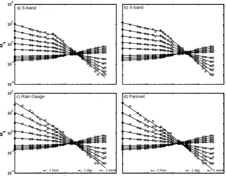
approximately 12 days. Because the finest temporal reso-lution of the data differs with instrument, we used 4.5 min averaged rain rates to compare the four instruments on the same time scales. In Fig. 7, we present the results from all instruments. As we can observe, there is a clear break in the scaling, common for all the calculated moments, at time scales around 2.4 h, which suggests that there are two differ-ent scaling regimes within the range of scales we investigated that govern the rainfall dynamics. This feature is more dis-tinct for the results from the VPRs. Olsson et al. (1993) ob-served similar breaks in the scaling of rainfall and suggested that these breaks correspond to characteristic time periods when changes in the temporal structure of the rainfall distri-bution occur. The average duration of wet periods in our data was 1.6 h with 1.5 h standard deviation.
994 E. I. Nikolopoulos et al.: Scaling analysis of rain data from collocated instruments
10-4 10-2 100 102 104
Mq a) S-band
10-4 10-2 100 102 104
λ
Mq
c) Rain Gauge
•← 1 hour •← 1 day •← 1 week
b) X-band
λ
d) Parsivel
•← 1 hour •← 1 day •← 1 week 10-4
10-2 100 102 104
Mq a) S-band
10-4 10-2 100 102 104
λ
Mq
c) Rain Gauge
•← 1 hour •← 1 day •← 1 week
b) X-band
λ
d) Parsivel
•← 1 hour •← 1 day •← 1 week
Fig. 7. Log-log plot of moments Mq of order q versus the scaling factor λ. Moments were calculated for time scales starting at 4.5 minutes up to 47 days. Note the break in the slope around 2.4 hours that suggests the existence of two scaling regimes. The moments displayed (bottom to top) are of order q equal to 0.2, 0.4, 0.6, 0.8, 1.5, 2, 2.5, 3 and 3.5 respectively.
Fig. 7. Log-log plot of momentsMq of orderqversus the
scal-ing factorλ. Moments were calculated for time scales starting at 4.5 min up to 47 days. Note the break in the slope around 2.4 h that suggests the existence of two scaling regimes. The moments dis-played (bottom to top) are of orderqequal to 0.2, 0.4, 0.6, 0.8, 1.5, 2, 2.5, 3 and 3.5 respectively.
In Fig. 8, we present the results we obtained from the four instruments. For q<1.5, all the instruments are in excel-lent agreement, but forq>1.5 there is a clear difference be-tween the resulting K(q) curves from the ground sensors (rain gauge and disdrometer) and the remote sensors (S-band and X-band VPR), with the first having a much steeper curve compared to the two profilers. A steepK(q)curve means that the moments of the underlying process differ greatly with different scales. Thus, the results we obtained from the four instruments suggest that the rain rates derived from the ground sensors show higher variability. This is not surpris-ing if we consider the fact that the rain rates derived from the profiler’s measurements are obtained by averaging over a sampling volume much larger than the one of the ground sensors, which results in a smoother rain rate signal.
The K(q) curves for both profilers show highly linear behavior whereas bothK(q)that correspond to the ground sensors exhibit nonlinear behavior (at least at some extent). The reasons for the differences in the observedK(q)are not clear, but the fact that there are certain similarities between the ground sensors and the remote sensors suggests that the differences in sampling principles that characterize the two groups of sensors might be a possible cause. One can spec-ulate that the constant Marshall-Palmer Z-R relationship that we used to derive the rain rates from the VPR’s observations can have a significant effect in the scaling properties. In or-der to investigate this, we repeated the scaling calculations for the S-band data but this time instead of using a single Z-R we used a storm-based Z-Z-R derived from the disdrometer data. The results, shown in Fig. 8, suggest that although there
1 2 3 0
0.5 1 1.5 2
-K
(q
)
q G
D
S X
S*
Fig. 8. Scaling function K(q) versus moment of order q for S-band (S), X-band (X), Parsivel (D) and rain gauge (G). The calculation of K(q) was based on the 47 days of data and for time scales starting from 4.5 minutes until approximately 2.4 hours. The S* and S curves corresponds to rainrates derived from S-band data based on different storm-based Z-R relationships (derived from disdrometer) and a constant Marshall-Palmer Z-R, respectively.
Fig. 8. Scaling functionK(q)versus moment of orderqfor S-band
(S), X-band (X), Parsivel (D) and rain gauge (G). The calculation ofK(q)was based on the 47 days of data and for time scales start-ing from 4.5 min until approximately 2.4 h. The S∗and S curves corresponds to rainrates derived from S-band data based on differ-ent storm-based Z-R relationships (derived from disdrometer) and a constant Marshall-Palmer Z-R, respectively.
is some effect of the different Z-Rs, it cannot explain the big difference between ground and remote sensors.
Since the above analysis was based on all 47 days of data, the scaling properties we derived result from a “mixing” of different storm events. In order to investigate the dependence of the derived scaling properties with the storm event as well as the differences between the instruments with storm event, we continued our analysis on a storm basis. We followed exactly the same methodology we described above for the same 6 storms we used for the autocorrelation analysis.
-0.2 -0.1 0 0.1 0.2 0.3 0.4 0.5 -K (q )
May 11, 2002 (Stratiform)
-0.2 -0.1 0 0.1 0.2 0.3 0.4 0.5
May 25, 2002 (Stratiform)
-0.2 0 0.2 0.4 0.6 0.8 1 1.2 1.4 1.6 -K (q )
June 02, 2002 (mixed strat./conv.)
S X G D -0.5 0 0.5 1 1.5 2 2.5
June 04, 2002 (Deep Convective)
1 2 3
-0.4 -0.2 0 0.2 0.4 0.6 0.8 1 1.2 1.4
June 11, 2002 (mixed strat./conv.)
-K
(q
)
q
1 2 3
-0.4 -0.2 0 0.2 0.4 0.6 0.8 1 1.2 q June 13, 2002 (mixed strat./conv.) -0.2 -0.1 0 0.1 0.2 0.3 0.4 0.5 -K (q )
May 11, 2002 (Stratiform)
-0.2 -0.1 0 0.1 0.2 0.3 0.4 0.5
May 25, 2002 (Stratiform)
-0.2 0 0.2 0.4 0.6 0.8 1 1.2 1.4 1.6 -K (q )
June 02, 2002 (mixed strat./conv.)
S X G D -0.5 0 0.5 1 1.5 2 2.5
June 04, 2002 (Deep Convective)
1 2 3
-0.4 -0.2 0 0.2 0.4 0.6 0.8 1 1.2 1.4
June 11, 2002 (mixed strat./conv.)
-K
(q
)
q
1 2 3
-0.4 -0.2 0 0.2 0.4 0.6 0.8 1 1.2 q June 13, 2002 (mixed strat./conv.)
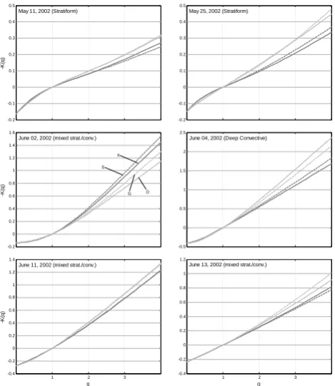
Fig. 9. Observed K(q) curves for the six storm events and for all instruments. Note that the y-axis scale is different in order to display the details of the curve’s shape.
Fig. 9. ObservedK(q)curves for the six storm events and for all
instruments. Note that the y-axis scale is different in order to display the details of the curve’s shape.
rainfall signal with lower extreme values than those recorded from the ground sensors. This explanation is reinforced by the fact that, in most cases, ground and remote sensors ex-hibit similar behavior.
The shape and magnitude of the observedK(q)curves dif-fer significantly with storm event (for all instruments), which suggests that scaling properties of rainfall depend strongly on rainfall type. Thus, it is somewhat inappropriate to try to de-rive the scaling characteristics of rainfall from the “mixing” of these storms. We did this in our initial approach by us-ing all 47 days of data, and although someone can use the results as an approximation of the scaling characteristics of rainfall, in our storm-based analysis we demonstrated that this approximation can sometimes differ significantly.
As the final step of our scaling analysis, we investigated the scaling properties of rainfall at different altitudes for stratiform and convective precipitation. We used the rain rates derived from the S-band and X-band VPR at 492, 2292, and 4392 m during the storm events of 25 May and 4 June 2002 that were mainly classified as stratiform and convec-tive, respectively. In Fig. 10, we present the calculatedK(q)
curves for both storms and for all altitudes.
For the stratiform event, theK(q)curves for S-band and X-band are almost identical at each height but they differ with height. More specifically, the K(q)curves appear to be steeper at the altitude of 2292 m (below the melting layer)
0 0.5 1 1.5
b) 4392 m
0 0.5 1 1.5
d) 2292 m
1 2 3
0 0.5 1 1.5
q f) 492 m
0 0.2 0.4 0.6 -K (q )
a) 4392 m
S-band X-band 0 0.2 0.4 0.6 -K (q )
c) 2292 m
1 2 3
0 0.2 0.4 0.6 -K (q ) q e) 492 m
0 0.5 1 1.5
b) 4392 m
0 0.5 1 1.5
d) 2292 m
1 2 3
0 0.5 1 1.5
q f) 492 m
0 0.2 0.4 0.6 -K (q )
a) 4392 m
S-band X-band 0 0.2 0.4 0.6 -K (q )
c) 2292 m
1 2 3
0 0.2 0.4 0.6 -K (q ) q e) 492 m
Fig. 10. Calculated K(q) curves based on rain rates derived from S-band and X-band data at three different altitudes, for the stratiform (May 25) and convective (June 04) storm event. Note that the y-axis scale is different between the stratiform (a), (c), (e) and convective (b), (d), (f) event. Fig. 10. CalculatedK(q)curves based on rain rates derived from
S-band and X-S-band data at three different altitudes, for the stratiform (25 May) and convective (4 June) storm event. Note that the y-axis scale is different between the stratiform (a), (c), (e) and convective (b), (d), (f) event.
than at 492 m (close to the ground), which suggests increas-ing variability with altitude, but at 4392 m (above the melt-ing layer) the variability decreases and results in a less steep
K(q)curve.
The convective event is associated with much steeper
K(q) curves, which is not surprising since it corresponds to what we currently know about the higher variability of convective precipitation. Moreover, we can observe that the
996 E. I. Nikolopoulos et al.: Scaling analysis of rain data from collocated instruments Our scaling analysis results might be subject to significant
uncertainty due to the small size of the sample of storms that we used. The impact of this issue is not well recognized in the literature and the potential problem is difficult to over-come as deployments of several collocated instruments are limited in time by duration of field experiments and funding. Still, since our emphasis is on the inter comparison of in-strumental ability to characterize rainfall, potential errors in some specific characteristics are of lesser importance.
5 Closing remarks and discussion
Technological advances in the field of rainfall studies over the last few decades have led to the development of such in-novative instruments as disdrometers, scanning radars, and profilers. Researchers utilize these new instruments to more effectively study several aspects of rainfall (e.g. estimation, statistical properties). However, all instruments are subject to a number of different sources of errors that introduce uncer-tainty in the estimates of rainfall and the properties derived from their observations. In this study, we investigated certain properties of rainfall and tried to explain central issues rela-tive to the instrumental-dependence of our results. Below, we summarize our main conclusions and discuss issues that require further investigation.
A number of factors (calibration, difference in temporal and spatial sampling etc.) must be considered in order to make a comparative analysis among different instruments meaningful. We addressed these issues and we described a methodology to account for most of them, but we acknowl-edge that there are still limitations regarding our approach (e.g. imperfect calibration and spatial matching).
Despite these differences between instruments, the results from the autocorrelation analysis showed very good agree-ment. This suggests that all instruments were able to cap-ture and represent the temporal variability of rainfall. The profilers allowed us to investigate this variability at a ver-tical extent and obtain useful information for the stratiform and convective types of precipitation. However, our spec-tral analysis results were based only on 2 storm events, and further analysis of more cases is therefore needed to verify a specific pattern of the temporal structure of rainfall in the stratiform and convective regimes.
The scaling investigation revealed certain similarities in the results from ground and remote sensors. Although we speculate that this is due to the differences in sampling vol-ume, further analysis is needed. A possible approach to demonstrate the effect of sampling volume would be to av-erage several sampling bins from the profiler data and repeat the scaling calculations. The storm-dependence of the differ-ences that was revealed suggests that the instruments do not represent all storms equally well, and although one would expect that the stratiform would show the best results, that was not always the case. One can argue that the storm-based
analysis is associated with the drawback of a small sample size and the effect that the few high values have to higher or-der moments can possibly explain the discrepancies observed but we observed distinct differences even forq≤2.
These differences also imply caution that one should use when attempting to translate results obtained in the time domain to the spatial domain. While vertically pointing radars provide more information about rainfall structure than ground-based in-situ devices such as rain gauges and dis-drometers, the fundamental issues in translating the temporal into spatial domain remain. For a discussion of these issues an interested reader is referred to Fabry (1996), for example.
Acknowledgements. The authors acknowledge support from
NSF Grant EAR-0409738. NOAA participation was supported
in part by a grant from the NASA Precipitation Measurement Mission. W. Krajewski acknowledges partial support of the Rose & Joseph Endowment.
Edited by: J. de Lima
Reviewed by: three anonymous referees
References
Atlas, D., Srivastava, R. C., and Sekhon, R. S: Doppler radar char-acteristics of precipitation at vertical incidence, Rev. Geophys. Space Phys., 11, 1–35, 1973.
Bras, R. L. and Rodriguez-Iturbe, I.: Random functions and hydrol-ogy, Reading, Massachusetts, Addison-Wesley Publishing Com-pany, 1985.
Ciach, G. J.: Local random errors in tipping-bucket rain gauge mea-surements, Adv. Water Resour., 22, 585–595, 2003.
Ciach, G. J. and Krajewski, W. F.: Analysis and modeling of spatial correlation structure of small-scale rainfall in Central Oklahoma, Adv. Water Resour., 29, 1450–1463, 2006.
Clark, W. L., Gage, K. S., Carter, D. A., Williams, C. R., Johnston, P. E., and Tokay, A.: Calibration issues using impact disdrom-eters for calibration of Doppler radar profilers, paper presented at 12th Symp. on Meteor. Observ. and Instrum., Amer. Meteor. Soc., California, abstract number P1.16, 2003.
de Lima, M. I. P. and Grasman, J.: Multifractal analysis of 15-min and daily rainfall from a semi-arid region in Portugal, J. Hydrol., 220, 1–11, 1999.
Fabry, F.: On the determination of scale ranges for precipitation fields, J. Geophys. Res., 101, 12 819–12 826, 1996.
Georgakakos, K. P., Carsteanu, A. A., Sturdevant, P. L., and Cramer, J. A.: Observation and analysis of Midwestern rain rates, J. Appl. Meteorol., 33, 1433–1444, 1994.
Habib, E. and Krajewski, W. F.: Uncertainty analysis of the
TRMM ground-validation radar-rainfall products: application to the TEFLUN-B field campaign, J. Appl. Meteorol., 41, 558–572, 2002.
Habib, E., Krajewski, W. F., Nespor, V., and Kruger, A.: Numeri-cal simulation studies of rain gauge data correction due to wind effect, J. Geophys. Res., 104, 19 723–19 734, 1999.
Harris, D., Seed, A., Menabde, M., and Austin, G.: Factors af-fecting multiscaling analysis of rainfall time series, Nonlin. Pro-cesses Geophys., 4, 137–156, 1997,
http://www.nonlin-processes-geophys.net/4/137/1997/.
Harris, D., Menabde, M., Seed, A., and Austin, G.: Breakdown co-efficients and scaling properties of rain fields, Nonlin. Processes Geophys., 5, 93–104, 1998,
http://www.nonlin-processes-geophys.net/5/93/1998/.
Hauser, D. and Amayenc, P.: Exponential Size Distributions of Raindrops and Vertical Air Motions Deduced from Vertically Pointing Doppler Radar Data Using a New Method, J. Appl. Me-teorol., 22, 407–418, 1983.
Kiely, G. and Ivanova, K.: Multifractal analysis of hourly precipi-tation, Phys. Chem. Earth (B), 24, 781–786, 1999.
Kitchen, M. and Blackall, R. M.: Representativeness errors in com-parisons between radar and gauge measurements of rainfall, J. Hydrol., 134, 13–33, 1992.
Kottegoda, N. T. and Rosso, R.: Statistics, Probability, and Relia-bility for Civil and Environmental Engineers, The McGraw-Hill Companies, Inc., 1997.
Krajewski, W. F. and Smith, J. A.: Radar Hydrology: rainfall esti-mation, Adv. Water Resour., 25, 1387–1394, 2002.
Krajewski, W. F., Ciach, G. J., and Habib, E.: An analysis of small-scale rainfall variability in different climatological regimes, Hy-drol. Sci. J., 48(2), 151–162, 2003.
Krajewski, W. F., Kruger, A., Caracciolo, C., Gol´e, P., Barthes, L., Creutin, J.-D., Delahaye, J.-Y., Nikolopoulos, E. I., Ogden, F., and Vinson, J.-P.: DEVEX-Disdrometer Evaluation Experiment: Basic results and implications for hydrologic studies, Adv. Water Resour., 29, 311–325, 2006.
Marshall, J. S. and Palmer, W.: The distribution of raindrops with size, J. Meteorol., 5, 165–166, 1948.
Muramoto K., Ebisu, S., Servomaa, H., Kubo, M., and Shiina, T.: Z-R Z-Relationship for Individual Snowfall and its Evaluation, SICE Annual Conference in Fukui, Japan, 2003.
Nikolopoulos, E. I.: Analysis of high resolution data of vertical structure of rainfall, M. S. thesis, Univ. of Iowa at Iowa City, Iowa, 2004.
Olsson, J., Niemczynowicz, J., and Berndtsson, R.: Fractal analy-sis of high-resolution rainfall time series, J. Geophys. Res., 98, 23 265–23 274, 1993.
Sieck, L. C., Burges, S. J., and Steiner, M.: Challenges in obtaining reliable measurements of point rainfall, Water Resour. Res., 43, W01420, doi:10.1029/2005WR004519, 2007.
Williams, C. R., Ecklund, W. L., and Gage, K. S.: Classification of precipitating clouds in the tropics using 915-MHz wind profilers, J. Atmos. Ocean. Tech., 12, 996–1012, 1995.
Williams, C. R., Johnston, P. E., Clark, W. L., Gage, K. S., Carter, D. A., and Kucera, P. A. Calibration of scanning radars using vertically pointing profilers and surface disdrometers, paper pre-sented at 12th Symp. on Meteor. Observ. and Instrum., Amer. Meteor. Soc., California, abstract number 11.3, 2003.