doi:10.5194/cp-7-511-2011
© Author(s) 2011. CC Attribution 3.0 License.
of the Past
Evaluating climate model performance with various parameter sets
using observations over the recent past
M. F. Loutre1, A. Mouchet2, T. Fichefet1, H. Goosse1, H. Goelzer3, and P. Huybrechts3
1Universit´e catholique de Louvain, Earth and Life Institute, Georges Lemaˆıtre Centre for Earth and Climate Research (TECLIM), Chemin du Cyclotron, 2 bte L7.01.11, 1348 Louvain-la-Neuve, Belgium
2Laboratoire de Physique Atmosph´erique et Plan´etaire, Universit´e de Li`ege, All´ee du 6 aoˆut, 17, Bˆatiment B5c, 4000 Li`ege, Belgium
3Earth System Science & Departement Geografie, Vrije Universiteit Brussel, Pleinlaan, 2, 1050 Brussels, Belgium Received: 6 April 2010 – Published in Clim. Past Discuss.: 29 April 2010
Revised: 19 April 2011 – Accepted: 20 April 2011 – Published: 17 May 2011
Abstract. Many sources of uncertainty limit the accuracy of climate projections. Among them, we focus here on the pa-rameter uncertainty, i.e. the imperfect knowledge of the val-ues of many physical parameters in a climate model. There-fore, we use LOVECLIM, a global three-dimensional Earth system model of intermediate complexity and vary several parameters within a range based on the expert judgement of model developers. Nine climatic parameter sets and three carbon cycle parameter sets are selected because they yield present-day climate simulations coherent with observations and they cover a wide range of climate responses to doubled atmospheric CO2concentration and freshwater flux perturba-tion in the North Atlantic. Moreover, they also lead to a large range of atmospheric CO2concentrations in response to pre-scribed emissions. Consequently, we have at our disposal 27 alternative versions of LOVECLIM (each corresponding to one parameter set) that provide very different responses to some climate forcings. The 27 model versions are then used to illustrate the range of responses provided over the recent past, to compare the time evolution of climate vari-ables over the time interval for which they are available (the last few decades up to more than one century) and to identify the outliers and the “best” versions over that particular time span. For example, between 1979 and 2005, the simulated global annual mean surface temperature increase ranges from 0.24◦C to 0.64◦C, while the simulated increase in atmo-spheric CO2 concentration varies between 40 and 50 ppmv. Measurements over the same period indicate an increase in
Correspondence to: M. F. Loutre ([email protected])
global annual mean surface temperature of 0.45◦C (Brohan
et al., 2006) and an increase in atmospheric CO2 concentra-tion of 44 ppmv (Enting et al., 1994; GLOBALVIEW-CO2, 2006). Only a few parameter sets yield simulations that re-produce the observed key variables of the climate system over the last decades. Furthermore, our results show that the model response, including its ocean component, is strongly influenced by the model sensitivity to an increase in atmo-spheric CO2 concentration but much less by its sensitivity to freshwater flux in the North Atlantic. They also highlight weaknesses of the model, in particular its large ocean heat uptake.
1 Introduction
Several strategies can be used to assess those uncertain-ties. Model results can be analysed to quantify the errors in the simulations. For example, Gleckler et al. (2008) pro-posed objective measures of coupled ocean-atmosphere gen-eral circulation model performance according to sevgen-eral cli-matic variables. They evaluate the model performance ac-cording to 2-D climatic fields simulated for a given climate state. Therefore, they calculate the root mean square (RMS) errors for each model and each variable using two references. They define a “typical” model error, i.e. the median of the RMS error calculations for each climatic variable, which is used to normalize the RMS error for each variable. So, they obtain a measure of how well a given General Circulation Model (GCM) compares with the typical model error. In parallel, the modelled responses to different external forc-ings are utilised to illustrate the uncertainty related to the non-perfect knowledge of the forcing (e.g. Crowley, 2000; Bertrand et al., 2002). Another example of strategy to as-sess model uncertainty is given by Murphy et al. (2004) and Stainforth et al. (2005). They used the same model and the same forcings with varied values of key physical parame-ters to identify the range of the climate response to a CO2 doubling related to parameter uncertainty. Lastly, Knutti et al. (2008) gave another example of strategy. Based on sev-eral emission scenarios and coupled GCMs, they concluded that the contribution of structural uncertainties (i.e. the error related to the choices made in the model structure that would remain even if all the parameters were perfectly known) to temperature projection over the next century is quite large (Knutti et al., 2008).
Among all those possible sources of uncertainty, we fo-cus here on the parameter uncertainty in LOVECLIM, a global three-dimensional Earth system model of intermedi-ate complexity (Goosse et al., 2010). The overall goal of this study is to design several alternative model versions that pro-vide a wide range of climate responses to a climate forcing. Therefore, we identify a reasonable number of parameter sets that yield present climate simulations coherent with observa-tions. Moreover, the various parameter sets should lead to a wide range of possible climate responses to increase in at-mospheric CO2 concentration and to freshwater discharge in the North Atlantic. They will thus provide a reason-able sample for quantifying the uncertainty of future climate changes in forthcoming studies. This approach has been cho-sen rather than a systematic random variation of important parameters because the latter would imply a very large num-ber of long simulations, which is not affordable even with a relatively fast model like LOVECLIM. Moreover, prelimi-nary tests clearly showed that most parameter combinations lead to unrealistic present-day climate and therefore would be useless for the purpose of this study. In addition, using a restricted number of parameter sets allows a better knowl-edge of their characteristics and thus potentially offers a bet-ter understanding of the different responses.
After a brief model description (Sect. 2), the remainder of the paper is divided into two major parts. First, we present the design of the alternative model versions (Sect. 3). Twenty-seven combinations of key physical parameter values of LOVECLIM that have a large impact on the model results are selected and utilised to carry out transient experiments over the last millennium. In the second part (Sect. 4), we use these model versions to analyse the range of responses to given forcings over the recent past. In particular, we focus on the ability of the model to simulate the trend of key global climate variables over the last century and, therefore, we de-sign a metric (i.e. a scalar measure) to quantify this ability. The last century was chosen because it corresponds to a pe-riod when relatively accurate observations are available for model-data comparison. Furthermore, as LOVECLIM has been (and is still) mainly used in process studies focused on mid- and high latitudes, we select variables that poten-tially have a direct or indirect impact on the evolution of sea level, on the stability of the North Atlantic meridional over-turning circulation (MOC) and on the future of the climate of polar regions. We also select global variables that give a global view on climate change. Therefore, in addition to atmospheric CO2concentration and surface temperature, we specifically assess the ability of the model to reproduce the observed trends in the Northern Hemisphere sea ice extent and global ocean heat content.
2 The climate model – description
LOVECLIM1.1 (further termed LOVECLIM) is a 3-D Earth System Model of Intermediate Complexity (EMIC). It con-sists of five components representing the atmosphere (EC-Bilt), the ocean and sea ice (CLIO), the terrestrial bio-sphere (VECODE), the oceanic carbon cycle (LOCH) and the Greenland and Antarctic ice sheets (AGISM). The ice sheet model AGISM (Huybrechts, 1990, 1996; Huybrechts and de Wolde, 1999) is not activated in this study because of the negligible influence of ice sheet-climate interactions on the climate evolution over the last century. Rather, its influ-ence on future climate simulations is investigated in a sepa-rate study (Goelzer et al., 2010). The previous model version (LOVECLIM1.0) is described in Driesschaert et al. (2007), while version 1.2, which differs only very slightly from ver-sion 1.1, is presented in Goosse et al. (2010).
0 500 1000 1500 Time
200 300 400 500 600
(ppmv)
Atmospheric CO2 concentration
0 200 400 600 800 1000 1200 1400 1600 1800 2000
Time (yr - arbitrary) 0
1 2 3 4 5
Global annual mean surface temperature (
o C)
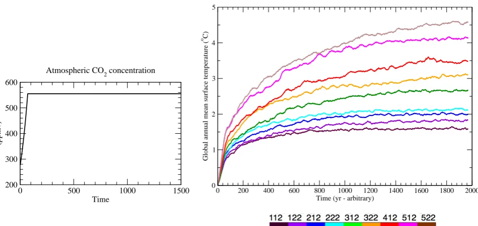
Fig. 1. Atmospheric CO2concentration in the perturbation scenario (left) and time evolution of the global annual mean surface temperature
in response to this perturbation according to the selected model parameter sets (right). Temperature is presented as deviation from the initial value. The colour code for the parameter sets is given in the figure.
VECODE (Brovkin et al., 2002) is a reduced-form model of the vegetation dynamics and of the terrestrial carbon cy-cle. It simulates the dynamics of two plant functional types (trees and grassland) at the same resolution as that of EC-BILT. LOCH (Mouchet and Franc¸ois, 1996; Mouchet, 2011) is a comprehensive oceanic carbon cycle model that includes an atmospheric module to represent the evolution of CO2, 13CO
2, and14CO2in the atmosphere. LOCH is fully cou-pled to CLIO and runs with the same time step and on the same grid. LOVECLIM has been utilised in a large num-ber of climate studies (e.g. Driesschaert et al., 2007; Goosse et al., 2007; Menviel et al., 2008a,b) and was part of several model intercomparison exercises (e.g. Braconnot et al., 2002, 2007a,b; Dutay et al., 2004).
3 Alternative model versions
3.1 Introduction – parameter sets
Several physical parameters of the model may significantly impact the model response to an external perturbation. We performed more than one hundred simulations using com-binations of parameters. These simulations were designed to lead to contrasted responses to a doubling of CO2 con-centration and to additional freshwater flux in the North At-lantic, and to induce different responses of the carbon cycle model. Amongst them, we selected those that produced rea-sonable simulations of the present-day climate. Eventually, we kept nine climatic parameter sets and three carbon cycle
parameter sets, which makes 27 parameter sets (see Sect. 1 of the Supplement for the description of the parameter sets; a three digit code identifies the parameter set, the first two digits correspond to the climatic parameter sets, and the third one to the carbon cycle parameter set).
3.2 Sensitivity
3.2.1 Sensitivity to CO2concentration
0 500 1000 1500 Time
0 0.05 0.1 0.15 0.2 0.25
(Sv)
Fresh water flux
0 200 400 600 800 1000 1200 1400 1600 1800 2000
Time (yr - arbitrary) 0
5 10 15 20 25 30
Maximum of overturning streamfunction - N. Atlantic (Sv)
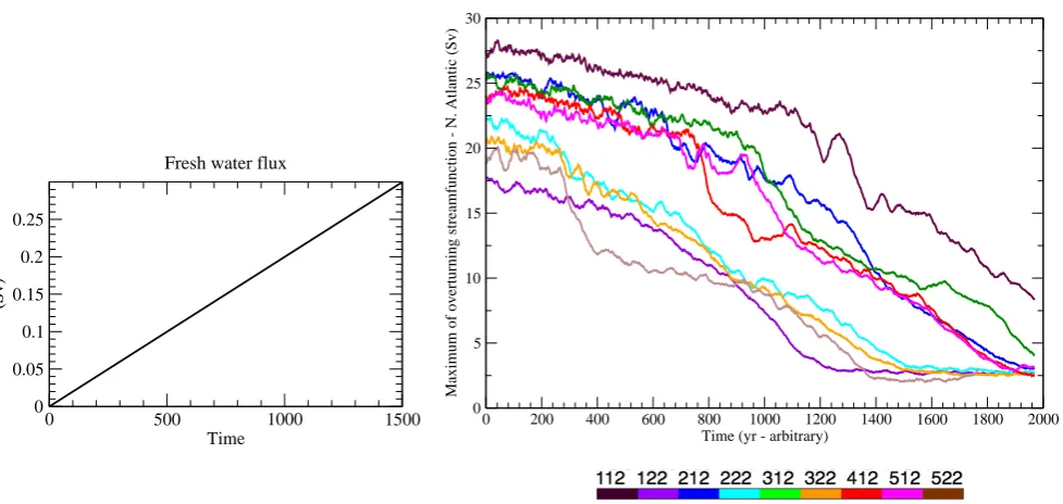
Fig. 2. Freshwater forcing in the North Atlantic in the perturbation scenario (left) and time evolution of the maximum of meridional overturning streamfunction below the Ekman layer in the Atlantic Ocean according to the selected model parameter sets in response to this perturbation (right). MOC is the absolute value. The colour code for the parameter sets is given in the figure.
(Fig. 1). This index represents the first digit that identifies the parameter sets.
The global annual mean surface temperature increase for the 9 climatic parameter sets ranges from 1.6 to 4.1◦C af-ter 1000 years (Table 2). Table 2 also provides the temper-ature increase after 70 years in the two times CO2scenario (i.e. the transient temperature response or TCR), the effective climate sensitivity (Ceff) computed according to Gregory et al. (2002) and the equilibrium climate sensitivity (Equi). The temperature increase after 1000 years in our sensitivity ex-periment (CS) is already very close to the value of the ef-fective climate sensitivity and the equilibrium climate sen-sitivity for the less sensitive parameter sets (112, 122, 212, and 222). Our parameters sets cover the likely range of cli-mate sensitivity suggested by the IPCC (Randall et al., 2007), i.e. 2.1◦C to 4.4◦C, based on GCM studies. It must be men-tioned that, although LOVECLIM using parameter set 112 is not exactly the same as LOVECLIM1.0 used in Driesschaert et al. (2007), it shares many climatic features with this for-mer version. In particular, its equilibrium sensitivity is rather low, i.e. 1.6◦C.
3.2.2 Sensitivity to water hosing
In a second sensitivity experiment (prefix E, suffix HYS, Ta-ble 1), freshwater is added in the North Atlantic (20 ˚ -50 ˚ N) with a linearly increasing rate of 2×10⁻⁴Sv yr−1. This re-sults in a freshwater perturbation of 0.1 Sv after 500 years, 0.2 Sv after 1000 years, and 0.3 Sv after 1500 years (Fig. 2, left). This simulation, which allows assessing the stability
Table 1. Summary of the major features of the different sensitivity simulations performed for each of the parameter sets (xyz). More details are given in the text.
Experiment name
Exyz Pre-industrial equilibrium (E-simulation): No volcanic forcing, GHG as in 1750, TSI = Total Solar Irradiance = 1365 Wm−2
Exyz2CO Two times CO2scenario:
Starting from the corresponding E-simulation
Forcings as in E-simulations except for the atmospheric CO2 concentration (Fig. 1).
ExyzHYS Water hosing simulation:
Starting from the corresponding E-simulation Forcings as in the E-simulations except for a freshwater perturbation applied in the North Atlantic (Fig. 2).
ExyzTRA Transient simulation from 1750 to 3000 starting from the corresponding E-simulation.
Forcings: orbital parameters, changes in concentration of GHGs other than CO2, anthropogenic emissions of CO2(both fossil fuel and deforestation fluxes).
112
122
212
222
312
322 412
512
522
1 1,5 2 2,5 3 3,5 4 4,5
Temperature increase for 2 X CO2 after 1000 years (oC) -60
-50 -40 -30 -20 -10 0
MOC decrease after 1000 years (%)
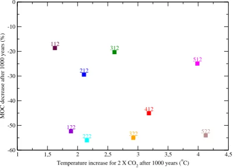
Fig. 3. Distribution of the model climatic parameter sets in the phase space (climate sensitivity, MOC sensitivity). The colour code for the parameter sets is also given below the figure.
is chosen to characterise the response of the model to this perturbation (MOC sensitivity). The MOC sensitivity is re-flected in the second digit of the name of the experiments: 1 for a decrease in the maximum value of the meridional overturning streamfunction of less than 50 %, and 2 other-wise. LOVECLIM with parameter set 112, i.e. the closest to LOVECLIM 1.0 used in Driesschaert et al. (2007), simulates a 20 % reduction in the meridional overturning streamfunc-tion after 1000 years. This decrease ranges from 19 to 56 % for the other parameter sets (Table 2).
Lastly, Fig. 3 confirms that the phase space (MOC sen-sitivity vs. climate sensen-sitivity) of our set of experiments is rather homogeneously covered as required by our initial ob-jective.
3.2.3 Sensitivity of the carbon cycle
We assess the sensitivity of the atmospheric CO2 level to the choice of carbon cycle parameters by performing a prog-nostic CO2experiment (prefix E, suffix TRA, Table 1) for each of the three parameter sets. This transient simulation starts from an equilibrium state corresponding to the con-ditions prevailing in 1750 AD (all years are in AD). It runs until year 3000 and is constrained by changes in the Earth orbital parameters (Berger, 1978) and in concentrations of greenhouse gases (GHGs) except CO2. In addition, the model is forced by anthropogenic emissions of CO2, includ-ing both fossil fuel and deforestation fluxes. Over the histori-cal period (1750–2000), the GHG concentrations (Houghton et al., 2001) and carbon emissions (Marland et al., 2003; Houghton, 2003) follow the historical records. From 2000 to 2100, we use the SRES A2 scenario (Houghton et al.,
Table 2. Main features of the model climate using different param-eter sets (first column).
Equilibrium
Name TCR CS Ceff Equi MOC MOC Ts
(1) (2) (3) (4) sensitivity (6) (7)
(5)
◦C ◦C ◦C ◦C % Sv ◦C
112 0.7 1.6 1.6 1.6 −19 28.4 16.1
122 0.8 1.9 1.9 2.0 −52 17.3 15.8
212 0.8 2.1 2.2 2.2 −29 25.6 15.8
222 0.9 2.2 2.2 2.3 −56 21.5 15.6
312 0.9 2.6 2.7 2.9 −20 25.1 16.4
322 1.0 2.9 3.1 3.3 −55 20.9 15.7
412 1.1 3.2 3.5 3.7 −45 24.0 15.9
512 1.5 4.0 4.4 4.5 −25 23.9 16.1
522 1.5 4.1 4.8 4.8 −54 19.9 15.5
(1) increase in global annual mean surface temperature after 70 years from the pre-industrial equilibrium value in the doubling CO2experiment;
(2) increase in global annual mean surface temperature after 1000 years from the pre-industrial equilibrium value in the doubling CO2experiment;
(3) the effective climate sensitivity according to Gregory et al. (2002) (see also Goelzer et al., 2010);
(4) the equilibrium response in global annual mean surface temperature is computed after 2000 years for the parameter sets 112, 122, 212, and 222; and after 3300 years for
the parameter sets 312, 322, 412, 512, and 522;
(5) percentage of decrease in the meridional overturning streamfunction after 1000 years in the water hosing experiment;
(6) strength of the meridional overturning streamfunction in the North Atlantic (Sv) at equilibrium in the pre-industrial experiment;
(7) annual mean global surface temperature (◦C) at equilibrium in the pre-industrial experiment.
2001) for both carbon emissions and GHG concentrations. After 2100, concentrations of all GHGs (except CO2) are kept fixed to their 2100 values, while CO2 emissions from land use are set to zero and fossil fuel emissions decrease ac-cording to a bell-shaped curve so that they reach zero a few decades after 2200 (Fig. 4, top left).
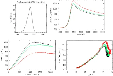
The three carbon cycle parameter sets (Table 3) lead to contrasted responses of the atmospheric CO2 to the identi-cal forcing (Fig. 4, top right). Maximal values of the atmo-spheric CO2concentration differ by up to 169 ppmv between carbon sets 1 and 3 (Table 3). By year 2500, they still differ by 133 ppmv, i.e. a relative difference of about 11 %. With carbon cycle parameter sets 1 and 2, the land CO2 uptake outpaces the ocean uptake (Fig. 4, bottom left), while the re-verse happens with carbon parameter set 3.
Anthropogenic CO2 emissions
1800 2000 2200 2400 0
5 10 15 20 25 30
Flux [GtC/yr]
1800 2000 2200 2400 2600 2800 3000
Year A.D. 200
400 600 800 1000 1200
Atm. CO
2
(
μ
atm)
0 500 1000 1500 2000
Ocean C (GtC) 0
200 400 600 800 1000 1200
Land C (GtC)
15 16 17 18 19 20
TS (
oC)
200 400 600 800 1000 1200
Atm. CO
2
(ppmv)
Fig. 4. CO2emission scenario (top, left) used to assess the sensitivity of the carbon cycle to the different carbon cycle parameter sets (see
description of the scenario in the text). It includes both fossil fuel emission and fluxes related to land use change. Evolution of the annual mean atmospheric CO2concentration (ppmv) with time (top, right), terrestrial carbon inventory versus ocean carbon inventory (both in GtC) (bottom, left), and atmospheric CO2versus the global annual mean surface temperature (bottom, right) for the different carbon cycle
parameter sets. The dashed line in the bottom left panel represents the 1:1 slope. Inventories are presented as anomalies with respect to the control run. The same colour code is used in each panel, i.e. black for parameter set 111, green for set 112, and red for set 113.
Table 3. Model parameter sets for the carbon cycle and their effect on the CO2response. These parameters influence the continental
vegetation fertilization effect (βgandβt; columns 2 and 3), the ver-tical flux of POM (αdiatomandαothers, columns 4 and 5), and the
buildup of calcium carbonate shells (9zoo, column 6). Columns 7
and 8 give the maximum value of the annual mean atmospheric CO2
concentration and its value at year 2500 from the transient simula-tions (see text) with the three carbon cycle parameter sets.
Carbon βg βt αdiatom αothers 9zoo Atm. CO2(ppmv)
parameter Max 2500
set AD
1 0.14 0.50 −0.750 −0.950 0.10 1146 877 2 0.36 0.36 −0.858 −0.858 0.22 1202 918 3 0.14 0.22 −0.648 −0.648 0.22 1315 1010
the maximum value of the atmospheric CO2range is about 10 %, while changes in oceanic remineralization depth ex-plain about three percent. Such small changes (a few ppmv) are within the variability produced by the model and can-not be ascertained yet. All together, the three parameter sets
allow us to obtain a change in the carbon climate sensitivity (as defined in Frank et al., 2010) of the order of 7 % (Fig. 4 bottom right).
The third digit in the experiment name refers to the carbon cycle parameter set with relatively low (1), medium (2), or high (3) changes in atmospheric CO2in response to the same emission scenario.
4 The climate of the last century
4.1 The simulations
1700 1800 1900 2000 Year AD
280 300 320 340 360
CO
2
concentration (ppmv)
1700 1800 1900 2000
Year AD 0
2 4 6 8
CO
2
emission (GtC/yr)
Fig. 5. Evolution over the last centuries (in year AD) of the atmospheric CO2concentration as prescribed in Conc (left) (Fl¨uckiger et al.,
2002; Monnin et al., 2004; Siegenthaler et al., 2005; Meure et al., 2006; Enting et al., 1994; GLOBALVIEW-CO2, 2006); and the emission of CO2(GtC yr−1) from fossil fuel burning as prescribed in Efor simulations (right) (Marland et al., 2003).
Table 4. Summary of the major features of the different simulations of the last millennium/century. The three digits xyz corresponds to the parameter set.
Experiment name
MxyzS1Conc Simulation of the last millennium climate (transient simulation): Starting from an equilibrium state at 500 AD.
Forcings∗: orbital parameters, land use changes, volcanic
activity, solar activity, changes in concentration of GHGs other than CO2, sulphate aerosols (S1), prognostic mode for atmospheric CO2concentration (CO2emissions are considered as a forcing).
MxyzS1Efor Simulation of the last millennium climate (transient simulation): Starting from an equilibrium state at 500 AD.
Forcings: orbital parameters, land use changes, volcanic activity, solar activity, changes in concentration of GHGs other than CO2, sulphate aerosols (S1), prognostic mode for atmospheric CO2 concentration (CO2emissions are considered as a forcing).
MxyzS2Conc Simulation of the last millennium climate (transient simulation): Starting from an equilibrium state at 500 AD.
Forcings: orbital parameters, land use changes, volcanic activity, solar activity, changes in concentration of GHGs other than CO2, sulphate aerosols (S2), diagnostic mode for atmospheric CO2 concentration (CO2concentration is considered as a forcing).
MxyzS2Efor Simulation of the last millennium climate (transient simulation): Starting from an equilibrium state at 500 AD.
Forcings: orbital parameters, land use changes, volcanic activity, solar activity, changes in concentration of GHGs other than CO2, sulphate aerosols (S2), prognostic mode for atmospheric CO2 concentration (CO2emissions are considered as a forcing).
∗The reader is referred to the text for a detailed explanation of the different simulations
and forcings.
of a simulation of the climate of the last century starting in 1900 from the state at 1900 of a climate simulation of the last millennium performed with the same parameter set (Sect. 3 of the Supplement). The members of one ensem-ble differ only in their initial conditions. To do so, we have
introduced a very small perturbation in the quasi-geostrophic potential vorticity the first day of the simulation, as described in Goosse et al. (2007).
The evolution of the atmospheric CO2concentration is ei-ther diagnostic or prognostic. In the diagnostic mode (Conc), the atmospheric CO2 concentration is prescribed according to Enting et al. (1994) until 1990, and then according to GLOBALVIEW-CO2 (2006) (Fig. 5). For the prognostic mode (Efor), the atmospheric CO2 concentration is com-puted by forcing the model with emissions of CO2from fos-sil fuel burning (Fig. 5, Marland et al., 2003). Both sim-ulations also take into account land use changes related to human activities as in Goosse et al. (2005) (percentage of crops; Ramankutty and Foley, 1999; Pongratz et al., 2008). We assume that croplands replace only forests, as long as there is a forest fraction. Furthermore, desert and forest (ex-cept for the part replaced by crops) keep their original extent at year 500. This scenario was previously used in a model intercomparison exercise aiming at analysing the response of six EMICs, including ECBilt-CLIO-VECODE, to historical deforestation (Brovkin et al., 2006).
In addition to the atmospheric CO2 concentration, either prescribed or computed by the model (see above, Enting et al., 1994; GLOBALVIEW-CO2, 2006; Marland et al., 2003), the transient simulations are forced by the volcanic activity (Crowley, 2000), the solar activity (Muscheler et al., 2007), the Earth orbital parameter changes (Berger, 1978; Bretagnon, 1982), and changes in concentrations of GHGs other than CO2 (Prather et al., 2001; Houghton et al., 1990 and updates).
76 78 80 82 84 86 88 90 92 94 CO2 concentration (ppmv)
0 0,1 0,2 0,3 0,4 0,5 0,6 0,7 0,8 0,9 1 1,1
Surface temperature (global annual mean - C)
76 78 80 82 84 86 88 90 92 94
CO
2 concentration (ppmv)
0 0.1 0.2 0.3 0.4 0.5 0.6 0.7 0.8 0.9 1 1.1
Surface temperature (global annual mean - C)
S2
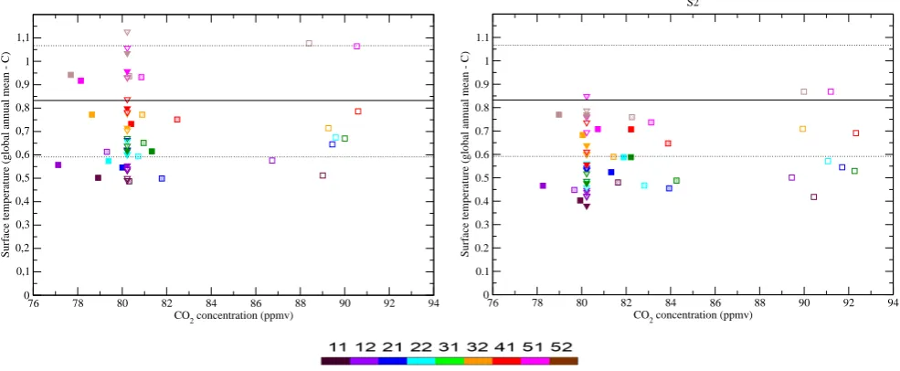
Fig. 6. Global annual mean surface temperature increase with respect to increase in atmospheric CO2 concentration. The mean value
increase is computed between the beginning of the 20th century (1901–1910) and the beginning of the 21st century (2000–2009). Values are averaged over five members of an ensemble. The left panel displays results for the S1 sulphate aerosol forcing. The sulphate aerosol forcing is doubled for the right panel (S2). The colour code refers only to the climatic parameter sets, i.e. the first two digits of the parameter set name. Full symbols are for carbon cycle parameter set 1, half-filled symbols are for carbon cycle parameter set 2, and empty symbols are for carbon cycle parameter set 3. The full name of the parameter set is obtained by appending the number corresponding to the carbon cycle parameter set (i.e. 1, 2, or 3 according to the symbol) to the number corresponding to the climate parameter set given by the colour code. Squares (triangles down) correspond to Efor (Conc) simulations. The vertical line of triangles representing the increase in atmospheric CO2
concentration in the scenario used for Conc-simulations also represents the best observation-based estimate of this increase. The full black line indicates the temperature increase over the 20th century as reconstructed by Brohan et al. (2006) (i.e. 0.83◦C). The dashed lines are the upper and lower 95 % uncertainty ranges.
its effect on the Earth climate is difficult to estimate. The radiative forcing computed by LOVECLIM for the present day with respect to the pre-industrial era related to the sul-phate aerosol load is−0.4 Wm−2in the reference situation (climatic parameter set 112). However, there is a large un-certainty in this quantity. IPCC AR4 (Forster et al., 2007) reported a direct radiative forcing due to sulphate aerosols of−0.40±0.2 Wm−2. The overall aerosol direct radiative forcing (i.e. radiative forcing values associated with several aerosol components) was estimated to−0.50±0.40 Wm−2. In addition to a direct effect, aerosol particles also affect the formation and properties of clouds. IPCC AR4 gives a me-dian value of−0.70 Wm−2 for the cloud albedo radiative forcing due to aerosol influence on clouds. Therefore, we decided to perform a second set of simulations for which the radiative forcing related to sulphates is doubled,−0.8 Wm−2 in the reference situation (climatic parameter set 112) (sce-nario S2).
4.2 Results
4.2.1 CO2concentration
The comparison of the simulated time evolution of the at-mospheric CO2concentration over the last century with data shows that some parameter sets display a poorer agreement than others (Fig. 6). In particular, the simulated increase in CO2 concentration obtained with carbon cycle parame-ter set 3 is of the order of 10 ppmv larger than in the cor-responding observations over the 20th century. In contrast, the simulated increase in atmospheric CO2concentration re-mains close to the measured one for carbon cycle parameter sets 1 and 2.
11 21 31 41 51 12 22 32 52 -0.1
-0.08 -0.06 -0.04 -0.02 0
(10
6 km 2 yr -1 )
Trend in minimum sea ice extent (data : bootstrap 1979-2006)
11 21 31 41 51 12 22 32 52
-0.1 -0.08 -0.06 -0.04 -0.02 0
(10
6km 2 yr -1)
Trend in minimum sea ice extent (data : bootstrap 1979-2006)
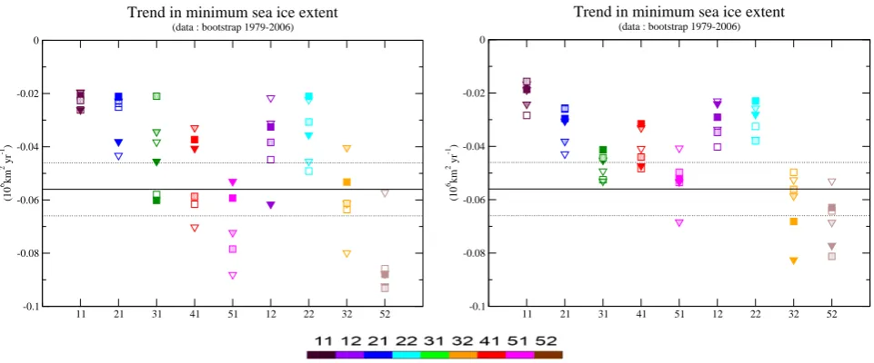
Fig. 7. Trend in minimum Northern Hemisphere sea ice extent between 1979 and 2006. X-axis is for the climate sensitivity, either for S1 (left) or S2 (right) sulphate aerosol forcing. The colour code refers only to the climatic parameter sets, i.e. the first two digits of the parameter set name. Full symbols are for carbon cycle parameter set 1, half-filled symbols are for carbon cycle parameter set 2, and empty symbols are for carbon cycle parameter set 3. The full name of the parameter set is obtained by appending the number corresponding to the carbon cycle parameter set (i.e. 1, 2 or 3, according to the symbol) to the number corresponding to the climate parameter set given by the colour code. Squares (triangles down) correspond to Efor (Conc) simulations. The full black line indicates the minimum sea ice extent as reconstructed by Comiso and Nishio (2008). The dashed line represents the uncertainty related to the variability in the data (one standard deviation on the slope).
observation series (Enting et al., 1994; GLOBALVIEW-CO2, 2006) over the time interval 1979–2005 yields simi-lar conclusions. For this period, the rate of increase in CO2 concentration varies between 1.48 and 1.62 ppmv yr−1 for carbon cycle parameter sets 1 and 2, respectively, with the S1 sulphate forcing. It is higher with the carbon cycle pa-rameter set 3 (between 1.71 and 1.79 ppmv yr−1). Here we obtain a larger CO2 increase for a smaller temperature in-crease, which can be considered as a negative CO2-climate feedback. In other words, the net feedback (Friedlingstein et al., 2003), which is the global warming amplification, is slightly smaller than one.
4.2.2 Surface temperature
The increasing trend in global annual mean surface temper-ature computed from HadCRUT3 time series (Brohan et al., 2006) is 0.0168◦C yr−1over the last 35 years (1979–2005) and 0.0071◦C yr−1over the last century (1901–2005). Some parameter sets lead to an underestimate of this increasing trend. This is, for example, the case for the climatic parame-ter sets 11, 21, and 22, especially with the S2 sulphate forc-ing; while other climatic parameter sets yield an overestimate of this trend, e.g. 51 and 52, especially with the S1 sulphate forcing.
4.2.3 Minimum sea ice extent
Most of the simulations, either with S1 or S2 sulphate aerosol forcing, experience a too small decrease in Northern Hemi-sphere minimum sea ice extent between 1979 and 2006 com-pared to observations (Fig. 7). This is especially the case for those simulations with low climate sensitivity (climatic pa-rameter sets 11, 12, 21, 22). For higher sensitivities, the type of simulation (Efor or Conc), the sulphate aerosol load (S1 or S2) as well as the sensitivity to the carbon cycle may play a role in the simulated trend. However, larger sulphate aerosol concentrations do not systematically lead to lower or higher trend in Northern Hemisphere minimum sea ice extent. 4.2.4 Oceanic variables
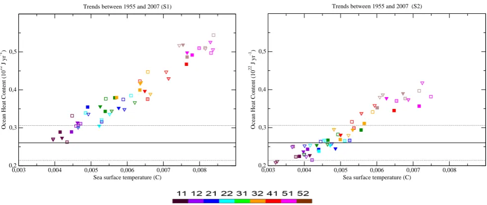
Most of the simulations overestimate the estimated warming of the global ocean in the 700 m upper layer over the last 50 years (Levitus et al., 2009) when the S1 sulphate forcing is used (Fig. 8). This overestimation is strongly reduced for S2 sulphate forcing. Indeed, in that case, only the simulations with high climate sensitivity (climatic parameter sets 51, 52, as well as 32 and 41 for some experimental setups) exhibit an ocean heat content increase significantly larger than in the real world.
0,003 0,004 0,005 0,006 0,007 0,008 Sea surface temperature (C)
0,2 0,3 0,4 0,5
Ocean Heat Content (10
22 J yr -1 )
Trends between 1955 and 2007 (S1)
0,003 0,004 0,005 0,006 0,007 0,008
Sea surface temperature (C) 0,2
0,3 0,4 0,5
Ocean Heat Content (10
22 J yr -1 )
Trends between 1955 and 2007 (S2)
Fig. 8. Trend in ocean heat content in the upper 700 m (1022J yr−1) wrt trend in sea surface temperature (C yr−1). Each symbol corresponds
to one simulation, either for S1 (left) or S2 (right) sulphate aerosol forcing. Trends are computed as the slope of the regression line through the annual values between 1955 and 2007. The colour code refers only to the climatic parameter sets, i.e. the first two digits of the parameter set name. Full symbols are for carbon cycle parameter set 1, half-filled symbols are for carbon cycle parameter set 2, and empty symbols are for carbon cycle parameter set 3. The full name of the parameter set is obtained by appending the number corresponding to the carbon cycle parameter set (i.e. 1, 2, or 3 according to the symbol) to the number corresponding to the climate parameter set given by the colour code. Squares (triangles down) correspond to Efor (Conc) simulations. The full black line represents the trend computed from observation (Levitus et al., 2009). The dashed line represents the uncertainty related to the variability in the data (one standard deviation on the slope of the linear regression through observation.
strength of North Atlantic MOC (AMOC) for S1 sulphate aerosol forcing (3 Sv; S2 sulphate aerosol forcing) (Fig. 9), although there is a large spread in the maximum intensity of the AMOC depending on the parameter sets (between 17 and 28 Sv in 1900 depending on the parameter).
4.2.5 Discussion
The surface temperature changes simulated over the last cen-tury obviously depend on the climate sensitivity. The pa-rameter sets corresponding to the lowest climate sensitivity (such as climatic parameter sets 11, 21, and 22) lead to small temperature changes over the last century and those with the largest climate sensitivity (e.g. climatic parameter sets 51 and 52) lead to a large temperature increase over the last century. Moreover, using a larger sulphate aerosol forcing tends to shift the simulated temperature increase over the last century towards smaller values because of the radiative cool-ing effect of those aerosols. Still, the discrepancy between simulated global annual mean surface temperature and ob-servations remains small (within one standard deviation) in many cases.
Moreover, although the deviation from observations of the simulated atmospheric CO2concentration is of the order of 10 ppmv over the 20th century (Fig. 6) for carbon cycle pa-rameter set 3, this discrepancy is not large enough to drive
the surface temperature towards larger values than for car-bon cycle parameter set 1 or 2. Therefore, most of the sim-ulations with carbon cycle parameter set 1 or 2 remain close to temperature observations, while those using carbon cycle parameter set 3 display only a small disagreement.
The simulations performed here display an approximately linear relationship between the increase in the upper ocean heat content and the increase in sea surface temperature (Fig. 8), i.e. when temperature increases, in particular sea surface temperature, the ocean captures more heat. We spec-ulate that a too large ocean heat uptake leads to a deficit in energy available at the ocean surface for melting the sea ice simulated with several parameter sets.
0 0,1 0,2 0,3 0,4 0,5 0,6 0,7 0,8 0,9 1 Sea surface temperature (global annual mean - C)
-5 -4 -3 -2 -1 0 1
Maximum of annual mean Atlantic meridional (NH) (Sv)
0 0.2 0.4 0.6 0.8 1
Sea surface temperature (global annual mean - C) -5
-4 -3 -2 -1 0 1
Maximum annual mean Atlantic meridional (NH) (SV)
S2
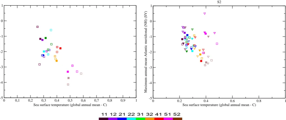
Fig. 9. Change in the maximum of the North Atlantic meridional overturning streamfunction (Sv) wrt change in the global annual mean sea surface temperature (◦C). The colour code refers only to the climatic parameter sets, i.e. the first two digits of the parameter set name, either for S1 (left) or S2 (right) sulphate aerosol forcing. Squares (triangles down) correspond to Efor (Conc) simulations. Full symbols are for carbon cycle parameter set 1, half-filled symbols are for carbon cycle parameter set 2, and empty symbols are for carbon cycle parameter set 3.
the 20th century than MOC sensitivity. In other words, even though we selected parameter sets in a large phase space, the ocean is responding more to the atmospheric forcing than to its intrinsic characteristics over the last few decades. The ini-tial states of the ocean, that are different depending on the pa-rameter sets, do not induce large changes in the upper ocean heat content either. Of course we should verify that this con-clusion, drawn only from LOVECLIM simulations, is robust for both other models and other forcings.
4.3 Performance of the parameter sets
Although none of the selected parameter sets is able to yield a climate simulation in the range of observations for all the variables examined, some parameter sets perform better than others. The purpose of this section is to characterise (and rank) them according to their performance. Therefore, we designed a metric that quantifies the ability of a simulation (i.e. a given parameter set and a given configuration) to sim-ulate the observed climate change over the last century. This metric is a measure of how well the simulated trends fit the observationally-based estimates of several climatic indica-tors during the 20th century. Indeed, as long as we are in-terested in climate change, it is more important to simulate a correct evolution of the variables, rather than a correct value of any time. The metric is based on the same variables as those discussed in the previous section (global annual mean surface temperature, atmospheric CO2concentration, mini-mum sea ice extent in the Northern Hemisphere, and ocean heat content of the upper 700 m of the global ocean). The
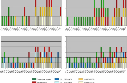
design of the metric is explained in Sect. 4 of the Supplement. Each simulation (i.e. given parameter sets, sulphate forcing, and setup) receives a score. None of the simulations received the maximum score of four (Conc) or six (Efor) points. The best simulations received a total score of three (Conc) and four (Efor) points (Fig. 10).
Simulations with the carbon cycle parameter set 3 do not properly reproduce the observed atmospheric CO2increase. Still, the deviation from observations remains less than 10 ppmv over the last 50 years and this does not prevent sim-ulation of temperature increase in agreement with observa-tions. Moreover, none can simulate simultaneously a correct time evolution for the ocean heat content in the upper 700 m and for the Northern Hemisphere sea ice extent. Goosse et al. (2007) studied the time evolution of the Northern Hemi-sphere sea ice extent in transient simulations from 8 kyr BP to 2100 AD, starting from an equilibrium state at 8 kyr BP, and using five parameter sets corresponding to 112, 212, 312, 412, and 512. They showed that, compared to obser-vations covering the second half of the 20th century, param-eter sets 112 and 212 seriously underestimate the decline in summer sea ice extent, while parameter set 312 slightly un-derestimates it. Therefore, Goosse et al. (2007) concluded that parameter sets 112 and 212 are incompatible with the observed record. This is well in line with our analysis.
0 1 2 3 4
0 1 2 3 4
0 1 2 3 4 5 6
0 1 2 3 4 5 6
Ocean heat uptake Sea ice extent
CO2 (1979‐2005)
CO2 (1901‐2005)
Ts (1979‐2005) Ts (1901‐2005)
Fig. 10. Summary of the performance of the Conc (top) and Efor (bottom) simulations to reproduce the observed trend of the time evolution for different climate variables for each parameter set under S1 (left) and S2 (right) sulphate aerosol forcings. The variables and the time intervals are described in Sect. 4 of the Supplement. The x-axis lists all the parameter sets. Colour bars indicate the variables (see colour code) simulated with a good skill (according to our metric), i.e.Rabove the threshold (see text). A single colour bar is used for sea ice and upper ocean heat content. Ts stands for global annual mean surface temperature either over the interval 1901–2005 or 1979–2005. CO2is
for atmospheric CO2concentration either over the time interval 1901–2005 or 1979–2005. Sea ice extent trend is computed either between 1979 and 2006 or 1979 and 2007. Trend in ocean heat content in the upper 700 m of the ocean is computed over either the time interval 1955–2007 or 1950–2003. See also the Supplement for references.
over the 20th century and the last decades is better simulated with S1 than S2.
When atmospheric CO2 concentration is prescribed (Conc), most of the parameter sets, except those with the lowest climate sensitivity, are able to reproduce the observed temperature trend over the 20th century. The trend in upper ocean heat content remains within 66 % of the median of the deviation from observations for the low climate sensitivity parameter sets when S1 aerosol forcing is used. It is also true for a few more parameter sets when S2 aerosol forcing is used.
Generally speaking, simulations with high climate sensi-tivity (climatic parameter sets 32, 41, 51, 52) have a better
global score than simulations with low climate sensitivity. Amongst the simulations ranking the highest (i.e. a final mark of 3 for Conc and 4 for Efor), parameter set 321 is the only one performing well for both Conc and Efor, as well as for both S1 and S2 sulphate aerosol forcings. Moreover, other parameter sets (322, 511, 512) also display good per-formance for both Conc and Efor, but only either for S1 or S2 sulphate aerosol forcing.
heat content in line with observations is also a major prob-lem for the other “good” parameter sets (except for parameter set 322 under Conc-setup with S2 sulphate aerosol forcing).
The difficulty of simulating properly the increase in the upper ocean heat content is a rather general feature of all the simulations, especially those with high climate sensitiv-ity. The parameter sets selected as having a “good skill” to reproduce the 20th century climate trend are those allowing a good simulation of the atmospheric temperature increase of the last century and the last decades of that century. How-ever, their skill in reproducing the increase in the upper ocean heat content is much poorer. Conversely, the parameter sets leading to a good representation of the trend in upper ocean heat content lead to a too weak global warming over the last century and last decades.
It is worth mentioning that a good skill over the last decades, as measured by the metric, does not guarantee a good skill over the entire last century. This is particularly true for the temperature changes for most of the parame-ter sets. On the other hand, as already underlined, most of the parameter sets do not allow accurately capturing the CO2 trend over the last decades, although the deviation is small. Moreover, Efor experiments have two additional degrees of freedom compared to Conc. In Efor, the atmospheric CO2 is prognostic as well as the carbon emissions resulting from the land-use changes, while, in Conc, the latter flux is im-posed and is the same for all climatic parameter sets. Since different climatic parameter sets lead to different vegetation distributions, the CO2emissions in Efor may differ among parameter sets. This results in different atmospheric CO2 levels, which in turn result in a different vegetation response since the latter also depends on CO2levels through the fertil-ization term. Lower atmospheric CO2concentration gener-ates a weaker carbon emission (and vice versa). Indeed, the emission is calculated on the basis of the potential growth of trees, which is favoured by higher atmospheric CO2 con-centrations. This may explain the change in performance be-tween Conc and Efor experiments, such as for parameter 412 (with S2 forcing), which is very poor in the Conc-simulation, while it performs well in the Efor-simulation.
For each variable, the metric gives only a binary result, either good or bad agreement between simulation and data. However, the discrepancy may be weak or strong, even for parameter sets that exhibit a good overall skill. For exam-ple, parameter set 321 (under Conc-setup), which has a good global score, displays a very strong disagreement for the upper ocean heat content with S1 sulphate aerosol forcing. Conversely, parameter set 211 displays a poor global skill, although the disagreement between model and data is only weak for most of the variables. This highlights how critical the choice of the threshold value is that separates between “good” and “poor” agreement.
5 Conclusions
This work is part of a study that aims at the quantification of uncertainties in modelling experiments used in climate change projections. Different approaches could be used, such as using various models or different external forcings. Here, we used different values for selected parameter sets of a particular model (LOVECLIM). In this way, we create alternative versions of the model. More precisely, we se-lected 27 parameter sets (nine climatic parameter sets and three carbon cycle parameter sets) according to their abil-ity (1) to cover a large range of potential climate behaviours over the next millennium, and (2) to properly simulate the major features of the present-day climate. This small and manageable number of parameter sets was selected because: (i) we broadly knew the individual effect of each parameter on the modelled climate; (ii) we knew that each parameter set would lead to realistic simulated present-day climate; and (iii) we knew for sure that they would yield a range of differ-ent model behaviours according to the model sensitivity to an increase in atmospheric CO2concentration, to its response to a freshwater hosing, and to its sensitivity to carbon cycle.
We designed a metric in order to quantify the skill of the different parameter sets to reproduce the climate change over the last decades of the 20th century, with a specific focus on global annual mean surface temperature, atmospheric CO2 concentration, minimum Northern Hemisphere sea ice ex-tent, and upper ocean heat content. Indeed, when designing this metric, we had in mind to simulate the evolution of the ice sheets and sea level in the future (Goelzer et al., 2010), and our metric is therefore based on variables chosen in line with this final purpose. However, another set of variables, for example giving more weight to the ocean or the ice sheet component of the system, could give rise to a slightly differ-ent conclusion about the skill of the parameter sets.
the simulation of past climates. Another possibility to be ex-plored is to give a weight to each simulation, with less weight given to a simulation performed with a low skill parameter set. However, in that case, additional simulations should be performed and more variables should be included in the de-sign of the metric.
We also noted that the climate sensitivity seems to have a stronger impact on the simulated climate, and even on the ocean behaviour, than the mean ocean state or the model re-sponse to a freshwater hosing. Of course, this conclusion ap-plies for LOVECLIM, within the framework of the forcing and parameter study performed here. It should be checked whether it is robust for other models, other parameterisations, or other forcings.
By using one single model, we did not address the struc-tural uncertainty (related to the choice made during the build-up of the model) that can also be a major source of discrep-ancy between model results. Ideally, both types of uncer-tainty should be addressed together, in addition to the ones associated with the forcing, but this long-term goal is clearly outside the scope of the present study. Even though we tested a large number of values for different key physical parame-ters of the model (many more than finally used in this study), we were unable to clearly solve identified drawbacks as un-derlined by some systematic biases present with all the pa-rameter sets, such as the strong ocean heat uptake. There-fore, we are convinced that further tuning will be relatively ineffective to improve the model behaviour to simulate past climates, at least for some variables and in some regions. Hence, improving the model probably requires improving the physics rather than (or in addition to) improving the values of its parameters. Given those biases, it is clearly inappropriate for the ensemble we have built to be used for making sound estimates of uncertainty in climate predictions/projections at the decadal-to-century time scale. Nevertheless, we feel that this ensemble is diverse and realistic enough to test the effect of the differences in model sensitivity, which are poorly con-strained and vary largely among GCMs and EMICs, on the long-term response of the Earth’s system to the greenhouse gas forcing. In Goelzer et al. (2010), for instance, it has been utilized to investigate the impact of fully interactive Green-land and Antarctic ice sheets under greenhouse warming con-ditions on the climate sensitivity at the millennial time scale. Supplementary material related to this
article is available online at:
http://www.clim-past.net/7/511/2011/ cp-7-511-2011-supplement.pdf.
Acknowledgements. The Belgian Federal Science Policy funded
this research within its Research Programme on Science for a Sus-tainable Development (SD/CS/01). We thank Pierre-Yves Barriat for helping in developments of the computer code. H. Goosse is Research Associate with the Fonds National de la Recherche Scientifique (Belgium). Computer time was partly made available
by UCL (Fonds sp´eciaux de recherche) and FNRS (Fonds de la recherche fondamentale collective) FRFC N 2.4502.05: “Sim-ulation num´erique. Application en physique de l’´etat solide, oc´eanographie et dynamique des fluides”. We thank Julia C. Har-greaves and two anonymous reviewers who provided helpful comments on the manuscript. We also thank the CISM-team.
Edited by: V. Rath
References
Berger, A.: Long-term variations of daily insolation and Quaternary climatic changes, J. Atmos. Sci., 35(12), 2362–2367, 1978. Bertrand, C., Loutre, M. F., Crucifix, M., and Berger, A.: Climate of
the last millennium: a sensitivity study, Tellus A, 54, 221–244, 2002.
Braconnot, P., Loutre, M. F., Dong, B., Joussaume, S., and Valdes, P.: How the simulated change in monsoon at 6 ka BP is related to the simulation of the modern climate: results from the Pale-oclimate Modeling Intercomparison Project, Clim. Dynam., 19, 107–121, 2002.
Braconnot, P., Otto-Bliesner, B., Harrison, S., Joussaume, S., Pe-terchmitt, J.-Y., Abe-Ouchi, A., Crucifix, M., Driesschaert, E., Fichefet, Th., Hewitt, C. D., Kageyama, M., Kitoh, A., Laˆın´e, A., Loutre, M.-F., Marti, O., Merkel, U., Ramstein, G., Valdes, P., Weber, S. L., Yu, Y., and Zhao, Y.: Results of PMIP2 coupled simulations of the MidHolocene and Last Glacial Maximum -Part 1: experiments and large-scale features, Clim. Past, 3, 261– 277, doi:10.5194/cp-3-261-2007, 2007a.
Braconnot, P., Otto-Bliesner, B., Harrison, S., Joussaume, S., Pe-terchmitt, J.-Y., Abe-Ouchi, A., Crucifix, M., Driesschaert, E., Fichefet, Th., Hewitt, C. D., Kageyama, M., Kitoh, A., Loutre, M.-F., Marti, O., Merkel, U., Ramstein, G., Valdes, P., We-ber, L., Yu, Y., and Zhao, Y.: Results of PMIP2 coupled simulations of the MidHolocene and Last Glacial Maximum -Part 2: feedbacks with emphasis on the location of the ITCZ and mid- and high latitudes heat budget, Clim. Past, 3, 279–296, doi:10.5194/cp-3-279-2007, 2007b.
Bretagnon, P.: Th´eorie du mouvement de l’ensemble des plan`etes. Solution VSOP82, Astron. Astrophys., 30, 141–154, 1982. Brohan, P, Kennedy, J. J., Harris, I., Tett, S. F. B., and Jones, P.
D.: Uncertainty estimates in regional and global observed tem-perature changes: a new dataset from 1850, J. Geophys. Res., 11(D12), D12106, doi:10.1029/2005JD006548, 2006.
Brovkin, V., Bendsten, J., Claussen, M., Ganopolski, A., Kubatzki, C., Petoukhov, V., and Andreev, A.: Carbon cycle, vegeta-tion and climate dynamics in the Holocene: Experiment with the CLIMBER-2 model, Global Biogeochem. Cy., 16(4), 1139, doi:10.1029/2001GB001662, 2002.
Brovkin, V., Claussen, V., Driesschaert, E., Fichefet, T., Kick-lighter, D., Loutre, M. F., Matthews, H. D., Ramankutty, N., Schaeffer, M., and Sokolov, A.: Biogeophysical effects of his-torical land cover changes simulated by six Earth system mod-els of intermediate complexity, Clim. Dynam., 26(6), 587–600, doi:10.1007/s00382-005-0092-6, 2006.
Comiso, J. C. and Nishio, F.: Trends in the Sea Ice Cover Us-ing Enhanced and Compatible AMSR-E, SSM/I, and SMMR Data, nsidc.org/data/smmr ssmi ancillary/area extent.html, last access: 19 August 2009, J. Geophys. Res., 113, C02S07, doi:10.1029/2007JC004257, 2008.
Crowley, T.: Causes of climate change over the past 1000 years, Science, 289, 270–277, 2000.
Driesschaert, E., Fichefet, T., Goosse, H., Huybrechts, P., Janssens, I., Mouchet, A., Munhoven, G., Brovkin, V., and Weber, S. L.: Modeling the influence of Greenland ice sheet melting on the meridional overturning circulation during the next millennia, Geophys. Res. Lett., 34, L10707, doi:10.1029/2007GL029516, 2007.
Dutay, J.-C., Jean-Baptiste, P., Campin, J.-M., Ishida, A., Maier-Reimer, E., Matear, R. J., Mouchet, A., Totterdell, I. J., Ya-manaka, Y., Rodgers, K., Madec, G., and Orr, J. C.: Evaluation of OCMIP-2 ocean models’ deep circulation with mantle helium-3. J. Mar. Syst., 48, 15–36, doi:10.1016/j.jmarsys.200helium-3.05.010, 2004.
Enting, I. G., Wigley, T. M. L., and Heimann, M.:
Fu-ture Emissions and Concentrations of Carbon Dioxide: Key Ocean/Atmosphere/Land Analyses, CSIRO Aust. Div. Atmos. Res. Tech. Pap., 31, 1–118, 1994.
Fl¨uckiger, J., Monnin, E., Stauffer, B., Schwander, J., Stocker, T. F., Chappellaz, J., Raynaud, D., and Barnola, J.-M.: High-resolution Holocene N2O ice core record and its relationship with CH4 and CO2, Global Biogeochem. Cy., 16(1), 1010,
doi:10.1029/2001GB001417, 2002.
Forster, P., Ramaswamy, V., Artaxo, P., Berntsen, T., Betts, R., Fa-hey, D. W., Haywood, J., Lean, J., Lowe, D. C., Myhre, G., Nganga, J., Prinn, R., Raga, G., Schulz, M., and Van Dorland, R.: Changes in Atmospheric Constituents and in Radiative Forc-ing, in: Climate Change 2007: The Physical Science Basis. Con-tribution of Working Group I to the Fourth Assessment Report of the Intergovernmental Panel on Climate Change, edited by: Solomon, S., Qin, D., Manning, M., Chen, Z., Marquis, M., Av-eryt, K. B., Tignor, M., and Miller, H. L., Cambridge University Press, Cambridge, UK and New York, NY, USA, 2007. Frank, D. C., Esper, J., Raible, C. C., B¨untgen, U., Trouet, V.,
Stocker, B., and Joos, F.: Ensemble reconstruction constraints on the global carbon cycle sensitivity to climate, Nature, 463, 527–532, doi:10.1038/nature08769, 2010.
Friedlingstein, P., Dufresne, J.-L., Cox, P. M., and Rayner, P.: How positive is the feedback between climate change and the carbon cycle?, Tellus B, 55, 692–700, 2003.
Gleckler, P. J., Taylor, K. E., and Doutriaux, C.: Performance met-rics for climate models, J. Geophys. Res., 113(D6), D06104, doi:10.1029/2007JD008972, 2008.
GLOBALVIEW-CO2: Cooperative Atmospheric Data Integration Project – Carbon Dioxide, CD-ROM, NOAA GMD, Boulder, Colorado, also available on Internet via anonymous FTP to ftp.cmdl.noaa.gov, Path: ccg/co2/GLOBALVIEW (last access: 15 September 2009), 2006.
Goelzer, H., Huybrechts, P., Loutre, M. F., Goosse, H., Fichefet, T., and Mouchet, A.: Impact of Greenland and Antarctic ice sheet interactions on climate sensitivity, Clim. Dynam., doi:10.1007/s00382-010-0885-0, in press, 2010.
Goosse, H. and Fichefet, T.: Importance of ice-ocean interactions for the global ocean circulation : A model study, J. Geophys.
Res., 104, 23337–23355, 1999.
Goosse, H., Crowley, T., Zorita, E., Ammann, C., Renssen, H., and Driesschaert, E.: Modelling the climate of the last millen-nium: What causes the differences between simulations?, Geo-phys. Res. Lett., 32, L06710, doi:10.1029/2005GL22368, 2005. Goosse, H., Driesschaert, E., Fichefet, T., and Loutre, M.-F.:
In-formation on the early Holocene climate constrains the summer sea ice projections for the 21st century, Clim. Past, 3, 683–692, doi:10.5194/cp-3-683-2007, 2007.
Goosse, H., Brovkin, V., Fichefet, T., Haarsma, R., Huybrechts, P., Jongma, J., Mouchet, A., Selten, F., Barriat, P.-Y., Campin, J.-M., Deleersnijder, E., Driesschaert, E., Goelzer, H., Janssens, I., Loutre, M.-F., Morales Maqueda, M. A., Opsteegh, T., Math-ieu, P.-P., Munhoven, G., Pettersson, E. J., Renssen, H., Roche, D. M., Schaeffer, M., Tartinville, B., Timmermann, A., and We-ber, S. L.: Description of the Earth system model of intermedi-ate complexity LOVECLIM version 1.2, Geosci. Model Dev., 3, 603–633, doi:10.5194/gmd-3-603-2010, 2010.
Gregory, J. M., Stouffer, R. J., Raper, S. C. B., Stott, P. A., and Rayner, N. A.: An observationally based estimate of the climate sensitivity, J. Climate, 15, 3117–3121, 2002.
Gregory, J. M., Dixon, K. W., Stouffer, R. J., Weaver, A. J., Driess-chaert, E., Eby, M., Fichefet, T., Hasumi, H., Hu, A., Jung-claus, J. H., Kamenkovich, I. V., Levermann, A., Montoya, M., Murakami, S., Nawrath, S., Oka, A., Sokolov, A. P., and Thorpe, R. B.: A model intercomparison of changes in the At-lantic thermohaline circulation in response to increasing atmo-spheric CO2 concentration, Geophys. Res. Lett., 32, L12703, doi:10.1029/2005GL023209, 2005.
Houghton, J. T., Jenkins, G. J., and Ephraums, J. J.: Climate Change: The IPCC Scientific Assessment, Cambridge Univer-sity Press, Cambridge, 365 pp., 1990.
Houghton, J. T., Ding, Y., Griggs, D. J., Noguer, M., van der Linden, P. J., Dai, X., Maskell, K., and Johnson, C. A.: Climate Change 2001:The Scientific Basis. Contribution of Working Group I to the Third Assessment Report of the Intergovernmental Panel on Climate Change, Cambridge University Press, 881p., 2001. Houghton, R. A.:. Revised estimates of the annual net flux of
car-bon to the atmosphere from changes in land use and land man-agement 1850–2000, Tellus B, 55(2), 378–390, 2003.
Huybrechts, P.: A 3-D model for the Antarctic ice sheet: a sensi-tivity study on the glacial-interglacial contrast, Clim. Dynam., 5, 79–92, 1990.
Huybrechts, P.: Basal temperature conditions of the Greenland ice sheet during the glacial cycles, Ann. Glaciol., 23, 226–236, 1996. Huybrechts, P. and de Wolde, J.: The dynamic response of the Greenland and Antarctic ice sheets to multiple-century climatic warming, J. Climate, 12, 2169–2188, 1999.
21, 2651-2663, doi:10.1175/2007JCLI2119.1, 2008.
Levitus, S., Antonov, J. I., Boyer, T. P. , Locarnini, R. A., Garcia, H. E., and Mishonov, A. V.: Global ocean heat content 1955–2008 in light of recently revealed instrumentation problems, Geophys. Res. Lett., 36, L07608, doi:10.1029/2008GL037155, 2009. Marland, G., Boden, T., and Andres, R.: Global, Regional, and
Na-tional Annual CO2Emissions from Fossil-Fuel Burning, Cement
Production, and Gas Flaring: 1751–2000, in : Trends: A com-pendium of data on global change, published by Carbon Dioxide Information Analysis Center, Oak Ridge, Tennessee, 2003. Meehl, G. A., Stocker, T. F., Collins, W. D., Friedlingstein, P., Gaye,
A. T., Gregory, J. M., Kitoh, A., Knutti, R., Murphy, J. M., Noda, A., Raper, S. C. B., Watterson, I. G., Weaver, A. J., and Zhao, Z.-C.: Global Climate Projections, in: Climate Change 2007: The Physical Science Basis. Contribution of Working Group I to the Fourth Assessment Report of the Intergovernmental Panel on Climate Change, edited by: Solomon, S., Qin, D., Manning, M., Chen, Z., Marquis, M., Averyt, K. B., Tignor, M., and Miller, H. L., Cambridge University Press, Cambridge, UK and New York, NY, USA, 2007.
Menviel, L., Timmermann, A., Mouchet, A., and Timm, O.: Meridional reorganizations of marine and terrestrial productiv-ity during Heinrich events, Paleoceanography, 23(1), PA1203, doi:10.1029/2007PA001445, 2008a.
Menviel, L., Timmermann, A., Mouchet, A., and Timm, O.: Climate and marine carbon cycle response to changes in the strength of the Southern Hemispheric westerlies, Paleoceanog-raphy, 23(4), PA4201, doi:10.1029/2008PA001604, 2008b. Meure, C. M., Etheridge, D., Trudinger, C., Steele, P., Langenfelds,
R., van Ommen, T., Smith, A., and Elkins, J.: Law Dome CO2,
CH4and N2O ice core records extended to 2000 years BP,
Geo-phys. Res. Lett., 3(14), L14810, doi:10.1029/2006GL026152, 2006.
Monnin, E., Steig, E. J., Siegenthaler, U., Kawamura, K., Schwan-der, J., Stauffer, B., Stocker, T. F., Morse, D. L., Barnola, J. M., Bellier, B., Raynaud, D., and Fischer, H.: Evidence for substantial accumulation rate variability in Antarctica during the Holocene, through synchronization of CO2in the Taylor Dome,
Dome C and DML ice cores, Earth Planet. Sc. Lett., 224(1–2), 45–54, doi:10.1016/j.epsl.2004.05.007, 2004.
Mouchet, A.: A 3D model of ocean biogeochemical cycles and cli-mate sensitivity studies. PhD thesis, Universit´e de Li`ege, Li`ege, Belgium, in preparation, 2011.
Mouchet, A. and Franc¸ois, L. M.: Sensitivity of a global oceanic carbon cycle model to the circulation and to the fate of organic matter: preliminary results, Phys. Chem. Earth, 21, 511–516, 1996.
Murphy, J. M., Sexton, D. M. H., Barnett, D. N., Jones, G. S., Webb, M. J., Collins, M., and Stainforth, A. A.: Quantification of mod-elling uncertainties in a large ensemble of climate change simu-lations, Nature, 430, 768–772, 2004.
Muscheler, R., Joos, F., Beer, J., Muller, S. A., Vonmoos, M., and Snowball, I.: Solar activity during the last 1000 yr inferred from radionuclide records, Quaternary Sci. Rev., 26(1–2), 82–97, 2007.
Nakicenovic, N. and Swart, R.: Special report on emissions scenar-ios, A special report of Working Group III of the Intergovern-mental Panel on Climate Change, Cambridge University Press, Cambridge, UK and New York, NY, USA, 599 pp., 2000.
NOAA ESRL: www.esrl.noaa.gov/gmd/ccgg/trends/ last access: 13 July, 2009.
Opsteegh, J. D., Haarsma, R. J., Selten, F. M., and Kattenberg, A.: ECBILT: A dynamic alternative to mixed boundary conditions in ocean models, Tellus A, 50, 348–367, 1998.
Pongratz, J., Reick, C., Raddatz, T., and Claussen, M.: A re-construction of global agricultural areas and land cover for the last millennium, Global Biogeochem. Cy., 22, GB3018, doi:10.1029/2007GB003153, 2008.
Prather, M., Ehhalt, D., Dentener, F., Derwent, R., Dlugokencky, E., Holland, E., Isaksen, I., Katima, J., Kirchhoff, V., Matson, P., Midgley, P., and Wang, M.: Atmospheric chemistry and green-house gases. In: Climate Change 2001: The Scientific Basis. Contribution of Working Group I to the Third Assessment Re-port of the Intergovernmental Panel on Climate Change, edited by: Houghton, J. T., Ding, Y., Griggs, D. J., Noguer, M., van der Linden, P. J., Dai, X., Maskell, K., and Johnson, C. A., Cam-bridge University Press, CamCam-bridge, UK and New York, NY, USA, 881 pp., 2001.
Rahmstorf, S., Crucifix, M., Ganopolski, A., Goosse, H., Ka-menkovich, I., Knutti, R., Lohmann, G., Marsh, B., Mysak, L., Wang, Z., and Weaver, A.: Thermohaline circulation hystere-sis: a model intercomparison, Geophys. Res. Lett., 32, L23605, doi:10.1029/2005GL023655, 2005.
Ramankutty, N. and Foley, J. A.: Estimating historical changes in global land cover: Croplands from 1700 to 1992, Global Bio-geochem. Cy., 13(4), 997–1027, 1999.
Randall, D. A., Wood, R. A., Bony, S., Colman, R., Fichefet, T., Fyfe, J., Kattsov, V., Pitman, A., Shukla, J., Srinivasan, J., Stouf-fer, R. J., Sumi, A., and Taylor, K. E.: Climate Models and Their Evaluation, in: Climate Change 2007: The Physical Science Basis. Contribution of Working Group I to the Fourth Assess-ment Report of the IntergovernAssess-mental Panel on Climate Change, edited by: Solomon, S., Qin, D., Manning, M., Chen, Z., Mar-quis, M., Averyt, K. B., Tignor, M., and Miller, H. L., Cam-bridge University Press, CamCam-bridge, UK and New York, NY, USA, 2007.
Siegenthaler, U., Monnin, E., Kawamura, K., Spahni, R., Schwan-der, J., Stauffer, B., Stocker, T. F., Barnola, J.-M., and Fis-cher, H.: Supporting evidence from the EPICA Dronning Maud Land ice core for atmospheric CO2 changes during the
past millennium, Tellus B, 57(7), 51–57, doi:10.1111/j.1600-0889.2005.00131.x, 2005.
Stainforth, D. A., Aina, T., Christensen, C., Collins, M., Faull, N., Frame, D. J., Kettleborough, J. A., Knight, S., Martin, A., Mur-phy, J. M., Piani, C., Sexton, D., Smith, L. A., Spicer, R. A., Thorpe, A. J., and Allen, M. R.: Uncertainty in predictions of the climate response to rising levels of greenhouse gases, Nature, 433, 403–406, doi:10.1038/nature03301, 2005.