www.clim-past.net/13/545/2017/ doi:10.5194/cp-13-545-2017
© Author(s) 2017. CC Attribution 3.0 License.
Assimilation of pseudo-tree-ring-width observations into
an atmospheric general circulation model
Walter Acevedo1,2, Bijan Fallah1, Sebastian Reich2, and Ulrich Cubasch1
1Institut für Meteorologie, Freie Universität Berlin, Carl-Heinrich-Becker-Weg 6–10, 12165 Berlin, Germany 2Institut für Mathematik, Universität Potsdam, Karl-Liebknecht-Strasse 24–25, 14476 Potsdam, Germany
Correspondence to:Bijan Fallah ([email protected])
Received: 14 September 2016 – Discussion started: 26 September 2016
Revised: 27 March 2017 – Accepted: 30 March 2017 – Published: 31 May 2017
Abstract.Paleoclimate data assimilation (DA) is a promis-ing technique to systematically combine the information from climate model simulations and proxy records. Here, we investigate the assimilation of tree-ring-width (TRW) chronologies into an atmospheric global climate model us-ing ensemble Kalman filter (EnKF) techniques and a process-based tree-growth forward model as an observation operator. Our results, within a perfect-model experiment setting, indi-cate that the “online DA” approach did not outperform the “off-line” one, despite its considerable additional implemen-tation complexity. On the other hand, it was observed that the nonlinear response of tree growth to surface temperature and soil moisture does deteriorate the operation of the time-averaged EnKF methodology. Moreover, for the first time we show that this skill loss appears significantly sensitive to the structure of the growth rate function, used to represent the principle of limiting factors (PLF) within the forward model. In general, our experiments showed that the error reduction achieved by assimilating pseudo-TRW chronologies is mod-ulated by the magnitude of the yearly internal variability in the model. This result might help the dendrochronology com-munity to optimize their sampling efforts.
1 Introduction
The low-frequency temporal variability in the climate sys-tem cannot be estimated from the available time span of instrumental climate records. Accordingly, paleoclimate re-construction must necessarily rely on the use of the paleo-climate proxy records. These natural archives exhibit sev-eral problematic features, e.g., low time resolution, sparse
and irregular spatial distribution, complex nonlinear response to climate, and high noise levels. Therefore the proper ex-traction of the climate signal contained therein can often re-main opaque (Evans et al., 2013). To date, many different ideas have been proposed in order to link proxy records to the paleoclimate conditions where they were created, e.g., data-driven statistical techniques, climate model hindcasts and Bayesian probabilistic methods (see Crucifix, 2012, for a recent review). Among this plethora of approaches, data assimilation (DA) methodologies are today particularly ap-pealing as they deliver estimates of paleoclimate quantities by systematically combining the information of paleoclimate records with the dynamical consistence of climate simula-tions (Brönnimann, 2011; Hakim et al., 2016).
So far, several very diverse paleo-DA schemes have been investigated, including pattern nudging (von Storch et al., 2000), forcing singular vectors (Barkmeijer et al., 2003; van der Schrier and Barkmeijer, 2005), 4D-Var (Paul and Schäfer-Neth, 2005; Kurahashi-Nakamura et al., 2014), par-ticle filters (Annan and Hargreaves, 2012; Dubinkina et al., 2011; Dubinkina and Goosse, 2013; Mathiot et al., 2013; Matsikaris et al., 2015) and ensemble Kalman filter tech-niques (EnKF; Huntley and Hakim, 2010; Bhend et al., 2012; Pendergrass et al., 2012; Steiger et al., 2014; see Hughes and Ammann, 2009; Widmann et al., 2010; Hakim et al., 2013 for further references).
the previous analysis state. This phenomenon, currently re-ferred to as an “off-line regime”, has been observed in several paleo-DA studies (Huntley and Hakim, 2010; Bhend et al., 2012; Pendergrass et al., 2012; Matsikaris et al., 2015). Fur-thermore, some recent studies have assumed the presence of the off-line condition and accordingly have removed the re-initialization step after assimilation altogether (Steiger et al., 2014; Dee et al., 2016; Hakim et al., 2016). These types of DA methodologies will be referred to in this paper as “off-line DA” techniques, in order to contrast them with tradi-tional “online DA” techniques, where the state of the model is updated after the assimilation of observations. Note that despite their lack of accumulation of observational informa-tion over time, off-line DA methodologies have already been shown to be more robust than traditional climate field recon-struction (CFR) techniques based on orthogonal empirical functions and stationarity assumptions (Steiger et al., 2014; Hakim et al., 2016).
A typical assumption in most of the paleo-DA stud-ies so far conducted is that the climate–proxy relation is linear. Nonetheless, currently it is widely recognized that climate proxies are the result of complex recording pro-cesses, which can be of a physical, chemical and biologi-cal nature. More realistic methodologies have been recently sculpted by the paleoclimate community in order to investi-gate the climate–proxy relationship, considering the distinct processes whereby the climate signal is recorded in proxy archives. Proxy forward modeling (Hughes et al., 2010; Evans et al., 2013) appears to be one of the most promis-ing methodologies in this area. In a proxy forward model the climate forcing is used as input data for producing the ar-tificial proxy records which can be directly compared with the actual ones. One application of proxy forward models is the prediction of the evolution of proxy archives (Vaganov et al., 2006). They can also be applied within climate re-construction strategies by using probabilistic inversion meth-ods like Bayesian hierarchical modeling (Tolwinski-Ward, 2012), Markov Chain Monte Carlo (MCMC) (Boucher et al., 2014) and DA (Hughes et al., 2010).
Several recent studies have investigated the applicabil-ity of process-based forward models in a paleo-DA set-ting (Hughes et al., 2010; Acevedo et al., 2015; Dee et al., 2016; Hakim et al., 2016). Acevedo et al. (2015) (AC15, hereafter) utilized the process-based tree-ring-width (TRW) forward model Vaganov–Shashkin Lite (VSL) (Tolwinski-Ward et al., 2011) and an online EnKF scheme to assimi-late pseudo-TRW records into a chaotic two-scale dynami-cal system. They found that the nonlinearities of the forward model may deteriorate the performance of the EnKF. Fur-thermore, they observed that this loss of skill may be ame-liorated by means of a fuzzy logic (FL)-based extension of the VSL model. Matsikaris et al. (2015) compared the off-line and onoff-line implementations of a “degenerate particle fil-ter” applied to a low-resolution Earth system model. They found similar skill for both methods on the continental and
hemispheric scales. Nonetheless, they concluded that in the off-line method the temporal consistency of the model is lost. On the other hand, Dee et al. (2016) used three differ-ent nonlinear proxy forward models (including VSL) and an off-line EnKF scheme to assimilate TRW, coral and ice core records into two different isotope-enabled atmospheric gen-eral circulation model (AGCMs). They demonstrated that the linear–univariate models for tree-ring width may not capture the AGCM’s climate, especially for regions where the tree’s growth is dominated by moisture.
This paper follows the rationale of AC15 but within a more realistic scenario, where an AGCM is used as a dy-namical system and the observational network resembles the currently available TRW chronologies. The purpose of this study is then to contribute to the present knowledge of paleo-DA techniques by addressing the following two questions:
i. Does the off-line regime naturally appear for the assim-ilation of TRW records into an AGCM?
ii. Is the FL-based extension of the VSL model still useful to improve the performance of a time-averaged EnKF technique when a climate model is used?
This study is structured as follows. In Sect. 2 we describe the DA technique, the TRW forward model and the climate model as well as the experimental setting used. Our numeri-cal results are shown in Sect. 3, followed by a discussion in Sect. 4.
2 Materials and methods
2.1 Data assimilation basics
In this paper, the term DA designates the process of estimat-ing the state of a system usestimat-ing observations and the physical laws governing the evolution of the system as represented in a numerical model (Talagrand, 1997). In a typical DA scheme, a dynamical model is integrated in time until ob-servations become available. Afterwards, the predicted state, also known as forecast, is “updated” using the observational information in order to obtain a corrected state, also known as the analysis. Finally, the model is re-initialized from the analysis state and propagated in time until the next assimila-tion time, completing the “analysis” cycle. DA methods have evolved from very empirical approaches, such as Newtonian relaxation, to probabilistic ones that attempt to estimate the probability density function (PDF) of the model state condi-tional on the observations (see Kalnay, 2003, Lahoz et al., 2010 and Reich and Cotter, 2015, for reviews).
EnKF’s implementation does not require any modification of the model’s code and uncertainty estimates can be di-rectly obtained from the ensemble spread (Hamill, 2006). The main disadvantage of EnKF, within a paleoclimate set-ting, is its inability to handle non-Gaussian PDFs, which can easily arise from the nonlinearities of climate models and observation operators. Recently, there have been several de-velopments in the field of nonlinear DA for high-dimension systems (Van Leeuwen et al., 2015); however, at the present fully non-Gaussian DA techniques are still prohibitively ex-pensive to run for general circulation climate models.
2.1.1 Kalman filter
Within the Kalman filter (KF) (Kalman, 1960), the PDF of forecast statep(x) is assumed to be given by a Gaussian func-tion with meanxf and covariancePf:
p(x)∝exp
−1 2
x−xfTPf−1x−xf
. (1)
The observationsy(tj) are also assumed to have Gaussian
errors and therefore the conditional probability of the obser-vation vectorygiven the statexis
p(y |x)∝exp
−1 2
y−bHxf
T
R−1y−bHxf
, (2)
wherebH is the observation operator andRis the observation
error covariance matrix. Following the Bayes theorem, the conditional probability of the state given the observations, i.e., the analysis PDF, is
p(x| y)∝exp
−1 2
x−xfTPf −1
x−xf
−1 2
y−bHxf
T
R−1y−bHxf
. (3)
Finally, assuming thatbH is a linear function,p(x| y) is also
a Gaussian function whose mean and covariance can be cal-culated by the Kalman update equations (Lorenc, 1986):
xa=xf+Ky−bHxf
, (4)
Pa= I−KbH
Pf, (5)
where the Kalman gain matrixKis given by:
K=PfbH†
b
HPfbH†+R
−1
. (6)
2.1.2 Ensemble Kalman filter
For realistic geophysical models, the dimensionality of the model state can be very high and then the calculation and storage of the covariance matrices can be prohibitively ex-pensive. A solution to this problem is provided by the EnKF
(Evensen, 1994), which uses an ensemble of model states (X(t)=(x1, . . .,xm)) to approximate KF equations.
Following this approach, the mean and covariance of the forecast take the following form:
hXfi =
1
m
m
X
i=1
xfi, Pf = 1
m−1X
0
f
Xf0T. (7)
Here X0f ∈Rn×m denotes the forecast ensemble deviation matrix:
X0f =Xf − hXfieT, (8)
wheree=(1, . . .,1)∈Rm. An analysis ensemble whose co-variance satisfies Eq. (5) can be generated in different ways, which can be classified into two main families: stochastic and deterministic filters (Hamill, 2006).
In the stochastic approach an observational ensembleYis generated by adding realizations of the observational noise to the observation vectory. The analysis ensemble is then created by the following update equation:
Xa=Xf +K Y−bHXf
. (9)
In the deterministic approach, instead of creating an ensem-ble of observations, the analysis mean and deviations are cal-culated using update formulae which do not involve random numbers (see Tippett et al., 2003 for further references).
A practical problem of EnKF schemes is that due to the limited ensemble size, the forecast uncertainty is usually un-derestimated. This leads to an excessive confidence in the forecast, and after several assimilation cycles the observa-tions may be completely ignored. This situation is normally avoided by means of an ad hoc procedure known as “covari-ance inflation”, where the forecast covari“covari-ance matrix is mul-tiplied by a constant greater than 1. Another undesired con-sequence of the limited ensemble size is that the ensemble state at any grid point will present non-negligible spurious correlations with observations located far apart in space. This difficulty is solved using another ad hoc procedure known as “covariance localization”. Here, we utilize the R localization (Hunt et al., 2007), where the entries of the observation error covariance matrix are multiplied by a function that increases exponentially with distance.
2.1.3 Time-averaged ensemble Kalman filter
its time-averaged part and the anomalies around it. After-wards, the original EnKF update formula is used to assim-ilate the time-averaged observations into the time-averaged forecast, obtaining the time-averaged analysis. Finally, the instantaneous analysis is form by adding the unaltered time-averaged forecast anomalies to the time-time-averaged analysis. This approach is based on the assumption that the observa-tions can only contain time-averaged information (Dirren and Hakim, 2005). If the time-averaged period is considerably longer than the timescales of the dynamical model, which may easily be the case for paleoclimate records, after assim-ilation the ensemble spread can reach climatological levels, leading to a complete lack of estimation skill for the forecast quantities. This behavior, currently referred to as the off-line regime, was first observed for the time-averaged EnKF ap-plied to a quasi-geostrophic atmospheric jet model (Huntley and Hakim, 2010; Pendergrass et al., 2012). Afterwards, sev-eral studies used the simplified off-line time-averaged EnKF approach with global climate models (Bhend et al., 2012; Steiger et al., 2014; Dee et al., 2016) assuming the presence of the off-line regime. However, to our knowledge, there had not been numerical evidence of the onset of off-line condi-tions for a full time-averaged EnKF algorithm applied to an AGCM. As mentioned in the introduction, filling this knowl-edge gap is one the objectives of this paper.
2.2 TRW forward model
The VSL model for TRW chronologies offers an intermediate-complexity approach between ecophysio-logical and completely data-driven models (Tolwinski-Ward et al., 2011; Tolwinski-Ward, 2012), where the climate-driven component of tree-ring growth is parameterized by way of a simple representation of the principle of limiting factors (PLF) (Fritts, 1976). The biological concept of PLF states that the pace at which a plant develops is controlled by the single basic growth resource, typically either energy or water, that is in shortest supply. Within VSL the limiting factors considered are near-surface air temperature (T) and soil moisture (M). These variables influence tree-ring growth via the “growth response” functions
gT=9
T−TL
TU−TL
(10)
and
gM=9
M−ML
MU−ML
, (11)
where9 is the piece-wise linear “standard ramp” function (Tolwinski-Ward et al., 2014)
9(u)=
0 if 0>u u if 0< u61 1 if u >1,
TLandMLdenote minimum thresholds for temperature and moisture below which there is no growth, andTU andMU
are upper thresholds above which tree growth is optimal. Af-terwards, the growth rateGMINis determined by the smallest
growth response, i.e.,
GMIN=min{gT, gM}. (12)
Finally, the yearly TRW valuesWare obtained by integrating in time the growth rate modulated by the relative insolation
I:
Wn=
tn Z
tn−τ
GMIN(t)I(t)dt. (13)
Herenstands for the number of the year,tnis the time at the
end of the yearnandτ is the length of the year (12 months). Regarding DA, VSL presents two challenging nonlinear aspects: (i) a “thresholded response” (Evans et al., 2013), arising from the insensitivity of trees to climate variability during dormancy and optimal growth, and (ii) “abrupt shift-ing of recorded variable” (Acevedo et al., 2015), comshift-ing from the structure of Eq. (12). There, the use of the minimum function implies that tree growth at a particular time can be limited by either temperature or moisture. Accordingly, tran-sitions between growth limitation regimes necessarily hap-pen in a sudden manner.
2.2.1 VSL from the fuzzy logic viewpoint
The term fuzzy logic was coined by Zadeh (1975) and refers to a mathematical theory which has been very successful in modeling complex systems involving imprecise data and vague knowledge of the underlying mechanisms. Since its in-troduction, FL has greatly influenced many disciplines, most notably control theory (Nguyen et al., 2002). Within the en-vironmental sciences, FL has been applied in ecological and hydrological modeling (Marchini, 2011; Salski, 2006; Se, 2009). Regarding climate proxy forward modeling, AC15 re-cently showed that the VSL model can be completely em-bedded into the framework of FL. Within this reinterpreta-tion, the growth response function gT (gM) corresponds to
the membership function to the setST(SM) of optimal
tem-perature (moisture) conditions for tree growth. Temtem-perature (moisture) values lying belowTL (ML) present null values
forgT(gM) and accordingly do not belong toST(SM). On the
other hand, temperature (moisture) values lying aboveTU
(MU) lead togT(gM) values equal to 1, meaning they belong
completely toST(SM). All the other temperature (moisture)
conditions present growth responses between 0 and 1, and consequently they are considered to belong partially toST
(SM). This idea of partial membership is the basis of fuzzy
logic and the sets defined this way are called fuzzy sets. Fur-thermore, the intersection of the fuzzy sets ST and SM is
calculated by evaluating the minimum betweenGTandGM:
gT∧M=min{gT, gM}. (14)
Equation (14) is completely equivalent to the Eq. (13). Then VSL’s growth rate function can be interpreted as the membership function for the fuzzy intersection setST∧M. In
FL theory, the minimum function (Eq. 14) is one of the most popular representations of the intersection operation; how-ever, it is not the only one as a whole family of appropriate functions actually exist referred to as t-norms (see Nguyen et al., 2002). In AC15 a number of t-norms was tested as replacement for VSL’s growth rate function within a highly simplified paleo-DA setting. In particular, it was found that the product t-norm gT∧M=gT·gM might significantly
im-prove the performance of the time-averaged EnKF technique. Accordingly, beside the minimum t-norm, we also consider the product growth response VSL-Prod in this paper:
GPROD=gT·gM. (15)
An important aspect of the product growth response VSL-Prod is the presence of an additional growth limitation regime where T and M concurrently limit tree-ring growth. This “co-limitation” regime allows a gradual transition be-tween temperature- and moisture-limited growth limitation regimes and accordingly a progressive alternation of the recorded variable. Growth co-limitation was initially recog-nized by Singh and Lal (1935), who called attention to the limitations of the original formulation of the PLF due to Blackman (1905). Within the ecological research commu-nity, co-limitation has been widely acknowledged as an cru-cial resource limitation phenomenon (Harpole et al., 2011), with abundant observational support both in terrestrial (Ni-inemets and Kull, 2005) and aquatic (Saito et al., 2008) envi-ronments. Interestingly, within the vegetation modeling com-munity the original PLF formulation is still the predominant approach to model photosynthesis (Yin and Struik, 2009).
2.3 Experimental design
Following the rationale used in the experiments of AC15, we conducted a set of DA experiments using the Simplified Pa-rameterizations, primitivE-Equation DYnamics (SPEEDY) model (Molteni, 2003) as a dynamical system and the VSL forward model as an observation operator. The time-averaged state of the atmosphere is estimated via the EnKF approach of Dirren and Hakim (2005). In the following, we describe in detail each of the components of our experimental setting.
2.3.1 Atmospheric general circulation model
The SPEEDY model (Molteni, 2003) is an intermediate-complexity atmospheric general circulation model (AGCM) comprising a spectral dynamical core and a set of simpli-fied physical parameterizations, based on the same princi-ples as state-of-the-art AGCM but tailored to work with just a
few vertical levels. Regarding the interaction with the ocean, SPEEDY offers two possible configurations: (i)prescribed ocean– sea surface temperature is directly imposed as forc-ing; (ii)slab ocean– the atmospheric model is coupled to a slab ocean model (qflux adjusted mixed layer model) forced by climatological ocean dynamics. Despite its low resolu-tion and the relatively low complexity of its parameteriza-tions, SPEEDY still captures many observed global climate features in a realistic way, while its computational cost is at least 1 order of magnitude lower than the one of sophisti-cated state-of-the-art AGCMs at the same horizontal resolu-tion (Molteni, 2003). The latter makes SPEEDY especially suitable for studies involving long ensemble runs, like the ones necessary for this study.
2.3.2 DA technique
The SPEEDY model was embedded by Miyoshi (2005) into the SPEEDY-LETKF framework, which offers a parallel im-plementation of a local ensemble transform Kalman filter (LETKF) (Hunt et al., 2007). Among the different types of EnKF, LETKF is particularly promising for high-resolution models given that the calculation of the analysis for a partic-ular grid point requires only the information of the neighbor-ing observations. Therefore, LETKF offers outstandneighbor-ing scal-ability properties. SPEEDY-LETKF is an open-source soft-ware which has already been used for several DA studies (Li et al., 2009; Miyoshi, 2010; Lien et al., 2013; Ruiz et al., 2013; Amezcua et al., 2014). Here, SPEEDY-LETKF was extended to allow the assimilation of pseudo-TRW obser-vations by means of either online or off-line time-averaged EnKF methods.
For the experiments presented in this paper, we employed ensembles of 24 members due to computational constraints. We used a constant multiplicative inflation of 1 % after the ensemble update and R localization via the following for-mula:
Rloc=R·exp (rh/2λh)2+(rv/2λv)2
, (16)
whererh and rv stand for the horizontal and vertical
dis-tances, respectively. Their corresponding scaling parameters were set to the values ofλh=500 km andλv=0.4 lnp.
2.3.3 Numerical experiments
Forecast Analysis
Ensemble DA method
Nature run
Pseudo-observations
Online DA (with cycling)
Ensemble members “True” trajectory
Free ensemble run Off-line DA (no cycling)
Observation operator
+ noise
Figure 1. Schematic of a typical observation system simulation experiment (OSSE) with ensemble online (with cycling) and off-line (no-cycling) DA methods.tdesignates the time axis andX(Y) denotes the model state (observation) space. Boxes with sharp (rounded) corners represent data (processes). Red (green) vertical bars indicate theforecast(analysis) spread. Vertical dotted lines rep-resent the assimilation steps.
dynamics.XFreeis intended to provide a benchmark of per-formance, against which it is possible to assess the added value of the DA scheme.
Initially, a 1-year-long spin-up run is performed starting from 1 January 1860. Afterwards, the final state of this model trajectory is used as the initial condition for a 150-year-long nature (“true”) run. The ensemble runs with and without DA are identically initialized from a set of states gathered from the last 2 months of the spin-up run (lagged 2-day initializa-tion). Note that the nature run and the different ensemble runs are generated with the same time-varying forcing fields. Re-garding the atmosphere–ocean coupling, we used SPEEDY’s slab ocean configuration, motivated by the fact that the slow variability in the slab ocean may lend predictability to the atmosphere. In these conditions, the online DA technique should have higher chances to outperform the off-line tech-nique.
Figure 2.Station set resembling real TRW network from Breiten-moser et al. (2014).
2.3.4 Observation generation
Pseudo-TRW observations are produced following VSL’s formulation plus a final white noise addition step, in which random draws from a Gaussian distribution are imposed on the time-averaged observations. Noise levels are assessed by means of the signal-to-noise ratio (SNR), given by the ra-tio of the standard deviara-tion of the unpolluted pseudo-TRW observations to the standard deviation of the additive white noise. Most of the results reported in Sect. 3 correspond to the optimistic value SNR=10, with the exception of the last sensitivity study, which analyzes the dependency on observa-tional noise levels. Regarding the geographical distribution of the observations, we place a pseudo-TRW chronology at every grid box where at least one actual TRW chronology from the database of Breitenmoser et al. (2014) is present. This strategy yields a realistic observational network com-prising 257 stations (see Fig. 2).
Concerning the configuration of the observation operator, we focus our study on the role of the growth rate function by configuring VSL in such a way that no thresholded response takes place. This is done by setting the upper and lower re-sponse thresholds to the maximum (minimum) values during the nature (true) run so that the response functions reduce to linear rescaling operators. We consider three different growth rate functions leading to three VSL configurations: (i) VSL-T, where the growth rate is directly given by the growth re-sponse to temperature (GT=gT); (ii) VSL-Min, where the
original “minimum” t-norm GMIN is used; and (iii)
VSL-Prod, where the FL-based “product” t-normGPROD is
uti-lized. Note that within the setup described above, VSL-T generates purely temperature-limited pseudo-chronologies, while VSL-Min and VSL-Prod generate mixed ones, where temperature and soil moisture determine tree-ring growth pace.
the leaky bucket model (LBM)1 (Huang et al., 1996), as it is normally done with the VSL model. Note that with the first option, the time series obtained present only intra-annual variability (yearly periodicity), while with the second option moisture time series do exhibit interannual variations.
2.3.5 Diagnostics
Thanks to the availability of the truth model evolution for our OSSEs, the forecast and analysis skill of the ensemble runs can be directly assessed. Given the annual resolution of TRW chronologies, we study the filter performance for yearly aver-aged values of near-surface temperatures. We focus our anal-ysis on near-surface temperature due to the larger error re-duction in this field as compared to other variables (e.g., hu-midity,uwind,v wind) when DA is applied. The behavior of ensemble runs is monitored by means of the root mean square error (RMSE) for the ensemble means. The results are shown as (1) time series of globally averaged tempera-ture RMSE, (2) histograms of these time series and (3) maps of time-averaged (150 years) temperature RMSEs.
3 Results
3.1 Unconstrained ensemble run
An AGCM is an example of a nonautonomous system, and accordingly the evolution of its state is determined by both the atmospheric dynamics and the external forcing. The in-fluences of these two distinct factors can be disentangled to some extent by considering atmospheric variability to be a superposition of an internal component, caused by the intrin-sic dynamics, and an external one, resulting from the vari-ations in the boundary conditions (Deza et al., 2014). Un-der this assumption, internal and external variability can be separated by way of a free ensemble run, using the ensem-ble mean as an estimate of the forced variability and the en-semble spread as an estimate of the internal variability. Fol-lowing this train of thought, Fig. 3a shows the magnitude of the yearly internal variability in near-surface temperature. Geographical regions around the Equator present negligible yearly internal variability, which can be explained by the fact that these areas are dominated by the daily cycle, and accord-ingly the 1-year-long averaging strongly attenuates their in-ternal variability. On the other hand, maximum spread values occur at high latitudes around±70◦. These yearly internal-variability maxima can be related to planetary-scale patterns fluctuating over timescales longer than 1 year, such as the “annular modes” (Thompson and Wallace, 2000) and dis-placements of the jet stream (Woollings et al., 2011). Regard-ing the error of the free ensemble run, Fig. 3b shows that the RMSE maxima clearly coincide with the internal-variability maxima, given that quantities without internal variability can
1The LBM code was extracted from VSL v2_3 (ftp://ftp.ncdc.
noaa.gov/pub/data/paleo/softlib/vs-lite/).
be well described by an ensemble run without DA. From that, it becomes clear that in our setting, DA can only be beneficial to estimate quantities displaying significant yearly internal variability.
3.2 Assimilating linear univariate time-averaged observations
In order to focus on the comparison between online and off-line DA techniques, we first consider the assimilation of temperature-limited pseudo-chronologies produced with VSL-T. Note that this observation operator generates linear univariate time-averaged observations, and accordingly the time-averaged EnKF must be in good conditions to operate, given that no nonlinearities are present in the observation op-erator.
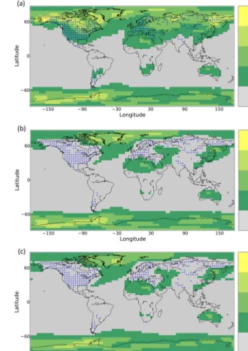
Figure 4b and c show how the assimilation effectively re-duces the error of the analysis for both online and off-line methods. All areas adjacent to the observational network show low RMSE values; however, it is important to high-light that stations located in areas of strong yearly internal variability are more efficient than the others at reducing the error of the analysis quantities. An example of this is the chronologies placed in Alaska, where RMSE reductions of up to 1.5◦take place. Conversely, stations situated in regions with weak yearly internal variability do no lead to significant error reductions, as is the case of the chronologies located in the Himalaya area, where SPEEDY presents no significant yearly temperature internal variability to be constrained via DA. Therefore, we claim that the error reduction for anal-ysis quantities is modulated by the magnitude of the yearly internal variability at a specific site.
On the other hand, online forecast quantities do not present significant error reductions, and consequently the online time-averaged EnKF appears to work under the off-line regime. This situation can be seen in Fig. 4a, which presents a strong resemblance with Fig. 3b, corresponding to the RMSE of the free ensemble run. Furthermore, looking at global RMSE time series (Fig. 5), it is evident that the errors for the online technique increase with time, as opposed to the corresponding off-line quantities, which presented stable be-havior all along the running time interval. Overall the off-line DA methodology leads to lower error levels on the global scale. The existence of this upward trend for online errors might be attributed to an undesired effect arising from the re-initialization of the ensemble after each assimilation step. For all our online DA experiments we observed the afore-mentioned lack of forecast skill. Consequently, for the rest of this section we will focus on the off-line DA technique.
3.3 Assimilating mixed TRW chronologies
(a)
E
Figure 3. Yearly near-surface temperature spread (a) and RMSE(b)for the free ensemble run.
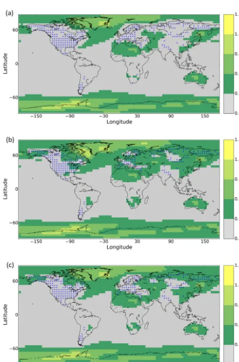
within the observation operator degrades the operation of the time-averaged EnKF, as it is illustrated by Fig. 6. Some ar-eas displaying very low RMSE values for VSL-T, such as Alaska, Siberia and central Asia, present considerably higher error levels when VSL-Min or VSL-Prod are utilized. This loss of skill to nonlinearities in the observation operator is also apparent in the global RMSE time series, as can be seen in Fig. 7, where VSL-T clearly outperforms the other two observation operators.
Regarding the dependency on the representation of the PLF, Fig. 6 shows that the use of VSL-Prod leads to con-siderably lower RMSE values in central Europe and the east coast of the United States. This edge of Prod over VSL-Min is also observed on the global scale, as can be seen in Fig. 7. These results concur with the ones of AC15, where in a highly simplified paleo-DA setting the use of VSL-Prod instead of VSL-Min appeared also beneficial to the perfor-mance of the time-averaged EnKF technique. Concerning the soil moisture fields, Fig. 8 shows how using the soil moisture calculated by the LBM reduces the error levels of both VSL-Min and VSL-Prod DA runs. However, these improvements in filter performance are more significant for VSL-Min than for VSL-Prod.
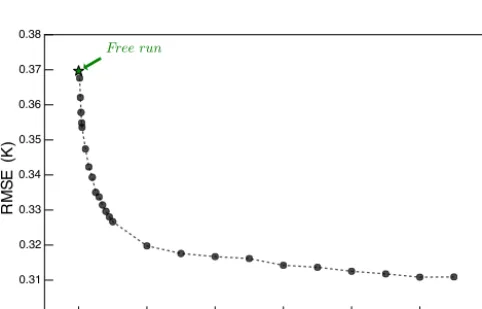
Finally, respecting the dependency of the filter perfor-mance on the observational noise levels, Fig. 9 shows how the off-line DA scheme is considerably effective for SNR values higher than 1. Increasing further the observational noise (reducing SNR) leads to a fast increase for the
aver-Figure 4.Yearly near-surface temperature RMSE for the ensemble run constrained by VSL-T pseudo-TRW observations.(a)Online forecast quantities,(b) online analysis quantities and(c)off-line analysis quantities
aged global RMSE curve, which reaches the error levels of a simulation without DA (free ensemble run) at SNR=0.03.
4 Conclusions
Using the time-averaged EnKF methodology and a process-based proxy forward model (VSL), we assimilated pseudo-TRW chronologies in an AGCM (SPEEDY). Using a set of perfect model experiments we studied two different aspects of the paleo-DA problem: (i) the onset of the off-line regime in the assimilation of observations averaged during long time periods and (ii) the impact of a nonlinear observation oper-ator on the performance of EnKF-based time-averaged DA approaches.
off-1900 1950 2000
0.2
0.3
0.4
0.5
Year
R
M
SE
Online−forecast
Online−analysis Free−forecastOnline−analysis
1900 1950 2000
0.2
0.3
0.4
0.5
Year
R
M
SE
R
M
SE
1900 1950 2000
0.2
0.3
0.4
0.5
Year
R
M
SE
(a)
0 5 10 15
0 5 10 15
0 5 10 15
D
Figure 5.Global near-surface temperature RMSE for the forecast ensemble run constrained by VSL-T pseudo-TRW observation (red) and the free ensemble run (black) for the analysis of online (green) and off-line (blue) DA. Panel (a)shows time series and panel(b)their corresponding histograms. Horizontal lines represent the mean values.
Figure 6. Yearly near-surface temperature RMSE for the anal-ysis of the ensemble runs using off-line DA and climatological soil moisture.(a)Assimilating VSL-T pseudo-TRW observations,
(b)assimilating VSL-Min pseudo-TRW observations and(c) assim-ilating VSL-Prod pseudo-TRW observations
1900 1950 2000
0.25
0.30
0.35
0.40
Year
RMSE
1900 1950 2000
0.25
0.30
0.35
0.40
Year
1900 1950 2000
0.25
0.30
0.35
0.40
Year
VSL−Min VSL−Prod VSL−T
(a)
0 5 10 15
0 5 10 15
0 5 10 15
E
Figure 7.Global near-surface temperature RMSE for the off-line analysis of the ensemble runs constrained by VSL-Min (red), VSL-Prod (green) and VSL-T (blue) pseudo-TRW observations. Climatological soil moisture is used to drive the VSL model. Horizontal lines represent the mean values. Panel(b)shows the histograms of the time series.
● ●
● ●
● ● ●
● ● ●
● ●
● ● ● ●
● ●
Free DA_Min DA_Min_LBM DA_Prod DA_Prod_LBM
0.25
0.30
0.35
0.40
0.45
0.50
0.55
RMSE
Figure 8.Global yearly near-surface temperature RMSE box plots for the free ensemble run forecast (free) and the analysis of the off-line DA runs using VSL-Min observation operator and climatolog-ical soil moisture (DA_MIN), VSL-Min observation operator and leaky bucket model (DA_MIN_LBM), VSL-Prod observation op-erator and climatological soil moisture (DA_PROD), and VSL-Prod observation operator and leaky bucket model (DA_PROD_LBM).
0 2 4 6 8 10 12
SNR 0.30
0.31 0.32 0.33 0.34 0.35 0.36 0.37 0.38
R
M
S
E
(
K
)
Freerun
Figure 9.Averaged global yearly near-surface temperature RMSE for the analysis of the ensemble run with off-line DA, VSL-Min observation operator and different signal-to-noise ratios. The green star shows the corresponding value for the free run.
time-averaged EnKF is its reliance on Gaussianity. This as-sumption might be easily violated in a climate model, for ex-ample by definite positive quantities such as humidity. Con-sequently non-Gaussianity might be also one of the culprits of the onset of the off-line regime in our experiments.
Concerning the influence of nonlinearities in the observa-tion operator, the performance of the off-line time-averaged EnKF appeared to be significantly sensitive to the selection of the t-norm used to represent the PLF. In our experiments, the product norm outperformed the original minimum t-norm, as previously observed for a two-scale Lorenz (1996) model in AC15. Tolwinski-Ward et al. (2014) described trees as fundamentally lossy2recorders of climate, due to the inte-grated nature of the information contained in them and the standardization process used to minimize the non-climatic effects on growth. In the same vein, we argue that the “abrupt shifting” of the recorded variable (temperature or moisture) – implied by the minimum function used in VSL’s original formulation – might constitute an additional source of lossi-ness, which can be reduced by resorting to an FL-based rep-resentation of the PLF. In particular, for the product t-norm, the existence of an additional co-limitation regime makes a smoother shifting of the recorded variable possible. As a cautionary remark, we want to highlight that the pseudo-observations assimilated in our experiments present several important limitations: (i) the thresholded response of trees to temperature and moisture was not considered in order to fo-cus on the role of the growth rate function; (ii) VSL’s param-eters were set in a completely homogeneous fashion for all the observational stations, whereas actual TRW networks are strongly heterogeneous, comprising chronologies generated under highly dissimilar growth limitation regimes. More re-alistic TRW assimilation experiments will probably have to
2This adjective is currently used in information technology to
address these issues as well as the necessity of considering model errors by conducting imperfect model OSSEs.
Finally, we want to mention that the translation of VSL into the FL language suggests other possible extensions for VSL. (i) Growth response functions can be generalized using the extensive knowledge on membership functions gathered in the FL research community (Nguyen et al., 2002). In par-ticular, it might be possible to tailor the shape of the growth response functions so as to optimize the performance of VSL regarding the particular application at hand, e.g., Gaussian DA, as was done in this paper. (ii) Additional limiting fac-tors, e.g., CO2concentration, can be easily incorporated into
the fuzzy inference system by adding new rules designed to express expert knowledge about the influence of these fac-tors on tree growth. (iii) The intrinsic uncertainty regarding VSLs parameters might be taken into account via the emerg-ing theory of stochastic FL (Luhandjula and Gupta, 1996). Furthermore, this ability of the FL approach to efficiently simulate complex processes involving vaguely understood mechanisms can be used in the development of new proxy forward models as well as in the extension of the existing ones.
Data availability. No data sets were used in this article.
Competing interests. The authors declare that they have no con-flict of interest.
Acknowledgements. This work was supported by the German Federal Ministry of Education and Research (BMBF) as part of the Research for Sustainable Development initiative (FONA; www.fona.de) through the PalMod project (FKZ: 01LP1511A). The computational resources were made available by the High-Performance Computing Center (ZEDAT) at Freie Universität Berlin and the German Climate Computing Center (DKRZ). Walter Acevedo wishes to acknowledge partial financial support by the Helmholtz graduate research school GeoSim.
Edited by: H. Goosse
Reviewed by: two anonymous referees
References
Acevedo, W., Reich, S., and Cubasch, U.: Towards the assimila-tion of tree-ring-width records using ensemble Kalman filtering techniques, Clim. Dynam., 46, 1909–1920, doi:10.1007/s00382-015-2683-1, 2015.
Amezcua, J., Ide, K., Kalnay, E., and Reich, S.: Ensemble trans-form Kalman-Bucy filters, Q. J.Roy. Meteor. Soc., 140, 995– 1004, doi:10.1002/qj.2186, 2014.
Annan, J. D. and Hargreaves, J. C.: Identification of climatic state with limited proxy data, Clim. Past, 8, 1141–1151, doi:10.5194/cp-8-1141-2012, 2012.
Barkmeijer, J., Iversen, T., and Palmer, T. N.: Forcing singular vec-tors and other sensitive model structures, Q. J. Roy. Meteor. Soc., 129, 2401–2423, doi:10.1256/qj.02.126, 2003.
Bhend, J., Franke, J., Folini, D., Wild, M., and Brönnimann, S.: An ensemble-based approach to climate reconstructions, Clim. Past, 8, 963–976, doi:10.5194/cp-8-963-2012, 2012.
Blackman, F. F.: Optima and limiting factors, Ann. Bot., 19, 281– 295, 1905.
Boucher, É., Guiot, J., Hatté, C., Daux, V., Danis, P.-A., and Dus-souillez, P.: An inverse modeling approach for tree-ring-based climate reconstructions under changing atmospheric CO2
con-centrations, Biogeosciences, 11, 3245–3258, doi:10.5194/bg-11-3245-2014, 2014.
Breitenmoser, P., Brönnimann, S., and Frank, D.: Forward mod-elling of tree-ring width and comparison with a global network of tree-ring chronologies, Clim. Past, 10, 437–449, doi:10.5194/cp-10-437-2014, 2014.
Brönnimann, S.: Towards a paleoreanalysis?, ProClim-Flash, 51, p. 16, 2011.
Burgers, G., van Leeuwen, P. J., and Evensen, G.: Analysis scheme in the ensemble Kalman filter, Mon. Weather Rev., 126, 1719– 1724, doi:10.1029/94JC00572, 1998.
Crucifix, M.: Traditional and novel approaches to
palaeo-climate modelling, Quaternary Sci. Rev., 57, 1–16,
doi:10.1016/j.quascirev.2012.09.010, 2012.
Dee, S. G., Steiger, N. J., Emile-Geay, J., and Hakim, G. J.: On the utility of proxy system models for estimating climate states over the common era, J. Adv. Model. Earth Syst., 8, 1164–1179, doi:10.1002/2016MS000677, 2016.
Deza, J. I., Masoller, C., and Barreiro, M.: Distinguishing the effects of internal and forced atmospheric variability in cli-mate networks, Nonlin. Processes Geophys., 21, 617–631, doi:10.5194/npg-21-617-2014, 2014.
Dirren, S. and Hakim, G. J.: Toward the assimilation of time-averaged observations, Geophys. Res. Lett., 32, L04804, doi:10.1029/2004GL021444, 2005.
Dubinkina, S. and Goosse, H.: An assessment of particle filtering methods and nudging for climate state reconstructions, Clim. Past, 9, 1141–1152, doi:10.5194/cp-9-1141-2013, 2013. Dubinkina, S., Goosse, H., Sallaz-Damaz, Y., Crespin, E., and
Crucifix, M.: Testing a particle filter to reconstruction climate over the past centuries, Int. J. Bifurcat. Chaos, 21, 3611–3618, doi:10.1142/S0218127411030763, 2011.
Evans, M. N., Tolwinski-Ward, S. E., Thompson, D. M., and An-chukaitis, K. J.: Applications of proxy system modeling in high resolution paleoclimatology, Quaternary Sci. Rev., 76, 16–28, doi:10.1016/j.quascirev.2013.05.024, 2013.
Evensen, G.: Sequential data assimilation with a nonlinear quasi-geostrophic model using Monte Carlo methods to fore-cast error statistics, J. Geophys. Res., 99, 10143–10162, doi:10.1029/94JC00572, 1994.
Fritts, H. C.: Tree rings and climate, Academic Press, New York, 1976.
Hakim, G. J., Emile-Geay, J., Steig, E. J., Noone, D., An-derson, D. M., Tardif, R., Steiger, N., and Perkins, W. A.: The last millennium climate reanalysis project: Framework and first results, J. Geophys. Res.-Atmos., 121, 6745–6764, doi:10.1002/2016JD024751, 2016.
Hamill, T. M.: Ensemble-based atmospheric data assimila-tion, in: Predictability of Weather and Climate, edited by: Palmer, T. and Hagedorn, R., Cambridge University Press, doi:10.1017/CBO9780511617652.007, 2006.
Harpole, W. S., Ngai, J. T., Cleland, E. E., Seabloom, E. W., Borer, E. T., Bracken, M. E., Elser, J. J., Gruner, D. S., Hille-brand, H., Shurin, J. B., and Smith, J. E.: Nutrient co-limitation of primary producer communities, Ecol. Lett., 14, 852–862, doi:10.1111/j.1461-0248.2011.01651.x, 2011.
Holton, J. and Hakim, G. J.: An Introduction to Dynamic Me-teorology, Academic Press, http://books.google.de/books?id= hLQRAQAAIAAJ, last access: 15 May 2017, 2013.
Huang, J., van den Dool, H. M., and Georgarakos, K. P.: Analysis of Model-Calculated Soil Moisture over the United States (1931–1993) and Applications to Long-Range Temper-ature Forecasts, J. Climate, 9, 1350–1362, doi:10.1175/1520-0442(1996)009<1350:AOMCSM>2.0.CO;2, 1996.
Hughes, M. and Ammann, C.: The future of the past – an earth system framework for high resolution paleoclimatology: edito-rial essay, Climatic Change, 94, 247–259, doi:10.1007/s10584-009-9588-0, 2009.
Hughes, M., Guiot, J., and Ammann, C.: An emerging paradigm: Process-based climate reconstructions, PAGES news, 18, 87–89, 2010.
Hunt, B. R., Kostelich, E. J., and Szunyogh, I.: Efficient data assimilation for spatiotemporal chaos: A local en-semble transform Kalman filter, Physica D, 230, 112–126, doi:10.1016/j.physd.2006.11.008, 2007.
Huntley, H. and Hakim, G.: Assimilation of time-averaged obser-vations in a quasi-geostrophic atmospheric jet model, Clim. Dy-nam., 35, 995–1009, doi:10.1007/s00382-009-0714-5, 2010. Kalman, R. E.: A New Approach to Linear Filtering and Prediction
Problems, J. Basic Eng.-T. ASME, 82, 35–45, 1960.
Kalnay, E.: Atmospheric modeling, data assimilation, and pre-dictability, Cambridge University Press, 2003.
Kurahashi-Nakamura, T., Losch, M., and Paul, A.: Can sparse proxy data constrain the strength of the Atlantic meridional overturning circulation?, Geosci. Model Dev., 7, 419–432, doi:10.5194/gmd-7-419-2014, 2014.
Lahoz, W., Khattatov, B., and Menard, R.: Data Assimilation: Making Sense of Observations, Springer, http://books.google.de/ books?id=KivkFpthm1EC, last access: 15 May 2017, 2010. Li, H., Kalnay, E., Miyoshi, T., and Danforth, C. M.: Accounting
for Model Errors in Ensemble Data Assimilation, Mon. Weather Rev., 137, 3407–3419, doi:10.1175/2009MWR2766.1, 2009. Lien, G.-Y., Kalnay, E., and Miyoshi, T.: Effective assimilation
of global precipitation: simulation experiments, Tellus A, 65, 19915, doi:10.3402/tellusa.v65i0.19915, 2013.
Lorenc, A. C.: Analysis methods for numerical weather
prediction, Q. J.Roy. Meteor. Soc., 112, 1177–1194,
doi:10.1002/qj.49711247414, 1986.
Lorenz, E. N.: Predictability, a problem partly solved, in: Proceed-ings of ECMWF Seminar on predictability, ECMWF, Reading, UK, 4–8 September 1995, 1–19, 1996.
Luhandjula, M K.. and Gupta, M. M.: On fuzzy stochastic op-timization, Fuzzy Set. Syst., 81, 47–55, doi:10.1016/0165-0114(95)00240-5, 1996.
Marchini, A.: Modelling Ecological Processes with Fuzzy Logic Approaches, in: Modelling Complex Ecological Dynamics, edited by: Jopp, F., Reuter, H., and Breckling, B., Springer Berlin Heidelberg, 133–145, 2011.
Mathiot, P., Goosse, H., Crosta, X., Stenni, B., Braida, M., Renssen, H., Van Meerbeeck, C. J., Masson-Delmotte, V., Mairesse, A., and Dubinkina, S.: Using data assimilation to investigate the causes of Southern Hemisphere high latitude cooling from 10 to 8 ka BP, Clim. Past, 9, 887–901, doi:10.5194/cp-9-887-2013, 2013.
Matsikaris, A., Widmann, M., and Jungclaus, J.: On-line and off-line data assimilation in palaeoclimatology: a case study, Clim. Past, 11, 81–93, doi:10.5194/cp-11-81-2015, 2015.
Miyoshi, T.: Ensemble Kalman filter experiments with a primitive-equation global model, PhD thesis, University of Maryland, Col-lege Park, 197 pp., 2005.
Miyoshi, T.: The Gaussian Approach to Adaptive Covariance In-flation and Its Implementation with the Local Ensemble Trans-form Kalman Filter, Mon. Weather Rev., 139, 1519–1535, doi:10.1175/2010MWR3570.1, 2010.
Molteni, F.: Atmospheric simulations using a GCM with simplified physical parametrizations. I: model climatology and variability in multi-decadal experiments, Clim. Dynam., 20, 175–191, 2003. Nguyen, H. T., Prasad, N. R., Walker, C. L., and Walker, E. A.: A First Course in Fuzzy and Neural Control, 1 Edn., Chapman and Hall/CRC, 2002.
Niinemets, Ü. and Kull, K.: Co-limitation of plant primary productivity by nitrogen and phosphorus in a species-rich wooded meadow on calcareous soils, Acta Oecol., 28, 345–356, doi:10.1016/j.actao.2005.06.003, 2005.
Paul, A. and Schäfer-Neth, C.: How to combine sparse proxy data and coupled climate models, Quaternary Sci. Rev., 24, 1095– 1107, doi:10.1016/j.quascirev.2004.05.010, 2005.
Pendergrass, A., Hakim, G., Battisti, D., and Roe, G.: Coupled Air-Mixed Layer Temperature Predictability for Climate Reconstruc-tion, J. Climate, 25, 459–472, doi:10.1175/2011JCLI4094.1, 2012.
Reich, S. and Cotter, C.: Probabilistic Forecasting and Bayesian Data Assimilation, in: Cambridge Texts in Applied Mathemat-ics, Cambridge University Press, https://books.google.de/books? id=xVpiCAAAQBAJ, last access: 1 May 2017, 2015.
Ruiz, J. J., Pulido, M., and Miyoshi, T.: Estimating Model Parame-ters with Ensemble-Based Data Assimilation: A Review, J. Me-teorol. Soc. Jpn., Ser. II, 91, 79–99, doi:10.2151/jmsj.2013-201, 2013.
Saito, M. A., Goepfert, T. J., and Ritt, J. T.: Some thoughts on the concept of colimitation: three definitions and the importance of bioavailability, Limnol. Oceanogr., 53, 276–290, 2008.
Salski, A.: Ecological Applications of Fuzzy Logic, in: Ecological Informatics, edited by: Recknagel, F., Springer Berlin Heidel-berg, 3–14, 2006.
Smith, D. M., Scaife, A. A., and Kirtman, B. P.: What is the current state of scientific knowledge with regard to seasonal and decadal forecasting?, Environ. Res. Lett., 7, 015602, doi:10.1088/1748-9326/7/1/015602, 2012.
Steiger, N., Hakim, G., Steig, E., Battisti, D., and Roe, G.: Assimi-lation of Time-Averaged Pseudoproxies for Climate Reconstruc-tion, J. Climate, 27, 426–441, doi:10.1175/JCLI-D-12-00693.1, 2014.
Talagrand, O.: Assimilation of observations, an introduction, Journal-Meteorological Society of Japan Series 2, 75, 81–99, 1997.
Thompson, D. W. J. and Wallace, J. M.: Annular Modes in the Extratropical Circulation. Part I: Month-to-Month Variability, J. Climate, 13, 1000–1016, doi:10.1175/1520-0442(2000)013<1000:AMITEC>2.0.CO;2, 2000.
Tippett, M. K., Anderson, J. L., Bishop, C. H., Hamill, T. M., and Whitaker, J. S.: Ensemble Square Root Fil-ters*, Mon. Weather Rev., 131, 1485–1490, doi:10.1175/1520-0493(2003)131<1485:ESRF>2.0.CO;2, 2003.
Tolwinski-Ward, S. E.: Inference on Tree-Ring Width and Paleo-climate Using a Proxy Model of Intermediate Complexity, PhD thesis, The University of Arizona, http://hdl.handle.net/10150/ 241975, last access: 22 May 2017, 2012.
Tolwinski-Ward, S. E, Tingley, M., Evans, M., Hughes, M., and Nychka, D.: Probabilistic reconstructions of local tempera-ture and soil moistempera-ture from tree-ring data with potentially time-varying climatic response, Clim. Dynam., 44, 791–806, doi:10.1007/s00382-014-2139-z, 2014.
Tolwinski-Ward, S. E., Evans, M. N., Hughes, M., and Anchukaitis, K. J.: An efficient forward model of the climate controls on in-terannual variation in tree-ring width, Clim. Dynam., 36, 2419– 2439, doi:10.1007/s00382-010-0945-5, 2011.
Vaganov, E., Hughes, M., and Shashkin, A.: Growth Dynamics of Conifer Tree Rings: Images of Past and Future Environ-ments, in: Ecological studies, Springer, New York, 183, 358 pp., doi:10.1007/3-540-31298-6, 2006.
van der Schrier, G. and Barkmeijer, J.: Bjerknes’ hypothesis on the coldness during AD 1790–1820 revisited, Clim. Dynam., 25, 537–553, doi:10.1007/s00382-005-0053-0, 2005.
Van Leeuwen, P. J., Cheng, Y., and Reich, S.: Nonlinear data assim-ilation, Springer, 2015.
von Storch, H., Cubasch, U., González-Ruoco, J., Jones, J., Wid-mann, M., and Zorita, E.: Combining paleoclimatic evidence and GCMs by means of data assimilation through upscaling and nudging (datun), in: Proceedings of the 11th Symposium on Global Change Studies, AMS, Long Beach, CA, USA, 9–14 Jan-uary 2000, 28–31, 2000.
Whitaker, J. S., Compo, G. P., and Thépaut, J.-N.: A Comparison of Variational and Ensemble-Based Data Assimilation Systems for Reanalysis of Sparse Observations, Mon. Weather Rev., 137, 1991–1999, doi:10.1175/2008MWR2781.1, 2009.
Widmann, M., Goosse, H., van der Schrier, G., Schnur, R., and Barkmeijer, J.: Using data assimilation to study extratropical Northern Hemisphere climate over the last millennium, Clim. Past, 6, 627–644, doi:10.5194/cp-6-627-2010, 2010.
Woollings, T., Pinto, J. G., and Santos, J. A.: Dynam-ical Evolution of North Atlantic Ridges and Poleward Jet Stream Displacements, J. Atmos. Sci., 68, 954–963, doi:10.1175/2011JAS3661.1, 2011.
Yin, X. and Struik, P.: C3 and C4 photosynthesis models: An overview from the perspective of crop modelling, NJAS-Wagen. J. Life Sc., 57, 27–38, doi:10.1016/j.njas.2009.07.001, 2009. Zadeh, L. A.: Fuzzy logic and approximate reasoning, Synthese, 30,