© Author(s) 2018. This work is distributed under the Creative Commons Attribution 4.0 License.
Application of ensemble transform data assimilation methods for
parameter estimation in reservoir modeling
Sangeetika Ruchi and Svetlana Dubinkina
Centrum Wiskunde & Informatica, P.O. Box 94079, 1098 XG Amsterdam, the Netherlands Correspondence:Sangeetika Ruchi ([email protected])
Received: 10 March 2018 – Discussion started: 23 March 2018
Revised: 21 September 2018 – Accepted: 17 October 2018 – Published: 6 November 2018
Abstract. Over the years data assimilation methods have been developed to obtain estimations of uncertain model parameters by taking into account a few observations of a model state. The most reliable Markov chain Monte Carlo (MCMC) methods are computationally expensive. Sequen-tial ensemble methods such as ensemble Kalman filters and particle filters provide a favorable alternative. However, en-semble Kalman filter has an assumption of Gaussianity. En-semble transform particle filter does not have this assumption and has proven to be highly beneficial for an initial condition estimation and a small number of parameter estimations in chaotic dynamical systems with non-Gaussian distributions. In this paper we employ ensemble transform particle filter (ETPF) and ensemble transform Kalman filter (ETKF) for parameter estimation in nonlinear problems with 1, 5, and 2500 uncertain parameters and compare them to importance sampling (IS). The large number of uncertain parameters is of particular interest for subsurface reservoir modeling as it allows us to parameterize permeability on the grid. We prove that the updated parameters obtained by ETPF lie within the range of an initial ensemble, which is not the case for ETKF. We examine the performance of ETPF and ETKF in a twin experiment setup, where observations of pressure are synthetically created based on the known values of param-eters. For a small number of uncertain parameters (one and five) ETPF performs comparably to ETKF in terms of the mean estimation. For a large number of uncertain parameters (2500) ETKF is robust with respect to the initial ensemble, while ETPF is sensitive due to sampling error. Moreover, for the high-dimensional test problem ETPF gives an increase in the root mean square error after data assimilation is per-formed. This is resolved by applying distance-based local-ization, which however deteriorates a posterior estimation of
the leading mode by largely increasing the variance due to a combination of less varying localized weights, not keeping the imposed bounds on the modes via the Karhunen–Loeve expansion, and the main variability explained by the leading mode. A possible remedy is instead of applying localization to use only leading modes that are well estimated by ETPF, which demands knowledge of which mode to truncate.
1 Introduction
An accurate estimation of subsurface geological properties like permeability and porosity is essential for many fields, especially where such predictions can have a large economic or environmental impact, for instance prediction of oil or gas reservoir locations. Knowing the geological parameters, a so-called forward model is solved for the model state and a prediction can be made. The subsurface reservoirs, how-ever, are buried thousands of feet below the Earth’s surface and exhibit a highly heterogeneous structure, which makes it difficult to obtain their geological parameters. Usually prior information about the parameters is given, which still needs to be corrected by observations of pressure and production rates. These observations are, however, known only at well locations that are often hundreds of meters apart and cor-rupted by errors. This gives instead of a well-posed forward problem an ill-posed inverse problem of estimating uncertain parameters, since many possible combinations of parameters can result in equally good matches to the observations.
methods with different perturbations and tested them on a 2-D reservoir model; Reynolds et al. (1996) obtained reser-voir parameter estimations using the Gauss–Newton method; Vefring et al. (2006) used the Levenberg–Marquardt method to characterize reservoir pore pressure and permeability. A review of history matching developments has been written by Oliver and Chen (2011).
For reservoir models the terms “data assimilation” and “history matching” are used interchangeably, as the goal of data assimilation is the same as that of history match-ing, where observations are used to improve a solution of a model. Ensemble data assimilation methods such as en-semble Kalman filters (Evensen, 2009) were originally de-veloped in meteorology and oceanography for the state es-timation. Now it is one of the frequently employed ap-proaches for parameter estimation in subsurface flow models as well (e.g., Oliver et al., 2008). A detailed review of en-semble Kalman filter developments in reservoir engineering is written by Aanonsen et al. (2009). An ensemble Kalman filter efficiently approximates a true posterior distribution if the distribution is not far from Gaussian, as it corrects only the mean and the variance. For nonlinear models with multi-modal distributions, however, an ensemble Kalman filter fails to correctly estimate the posterior, as shown by Dovera and Della Rossa (2011).
Importance sampling (IS) is quite promising for such mod-els as it does not have any assumptions of Gaussianity. It is also an ensemble-based method in which the probability density function is represented by a number of samples. One sample corresponds to one configuration of uncertain model parameters. The forward model is solved for each sample and predicted data are computed. The weight is assigned to sam-ples based on the observations of the true physical system and the predicted data. The drawback of IS is that it does not update the uncertain parameters, but only their weight; thus, a computationally unaffordable ensemble is required. In or-der to decrease this cost, a family of particle filters (Doucet et al., 2001) has been developed where IS is supplied with resampling, and a sample is called particle. Significant work for parameter estimation using particle filtering has been done in hydrology. Moradkhani et al. (2005) used it to es-timate model parameters and state posterior distributions for a rainfall–runoff model. Weerts and El Serafy (2006) com-pared an ensemble Kalman filter and a particle filter with dif-ferent resampling strategies for a rainfall–runoff forecast and found that as the number of particles increases, the particle filter outperforms the ensemble Kalman filter. Guingla et al. (2012) employed particle filtering to correct the soil moisture and to estimate hydraulic parameters.
The resampling in particle filtering is, however, stochastic. Ensemble transform particle filter (ETPF) developed by Re-ich and Cotter (2015) is a particle filtering method that de-terministically resamples the particles based on their weights and covariance maximization among the particles. ETPF has been used for initial condition estimations and for parameter
estimations in chaotic dynamical systems with a small num-ber of uncertain parameters (Lorenz 63 model). It has not been applied, however, in subsurface reservoir modeling for estimating a large number of uncertain parameters. In this pa-per we employ it for estimating uncertain parameters in sub-surface reservoir modeling. ETPF provides the equations that are solved in the space defined by the ensemble members. Therefore for comparison we employ the ensemble transform Kalman filter (ETKF) developed by Bishop et al. (2001) that also transforms the state from the model space to the ensem-ble space, minimizes the uncertainty in the ensemensem-ble space, and transforms the estimation back to the model space.
In this paper we investigate the performance of ETPF and ETKF for parameter estimation in nonlinear problems and compare them to IS with a large ensemble. This paper is orga-nized as follows: in Sect. 2 we describe IS, ETPF, and ETKF for parameter estimation. We apply these methods in Sect. 3 to a one-parameter nonlinear test case, where the posterior can be computed analytically, and in Sect. 4 to a single-phase Darcy flow, where the number of parameters is 5 and 2500. In Sect. 5 we draw the conclusions.
2 Data assimilation methods
We implement an ensemble transform Kalman filter and an ensemble transform particle filter for estimating parameters of subsurface flow. Both of these methods are based on a Bayesian framework. Assume we have an ensemble ofM model parameters{um}Mm=1; then, according to this frame-work, the posterior distribution, which is the probability dis-tributionπ(um|yobs)of the model parametersumgiven a set
of observationsyobs, can be estimated by the pointwise mul-tiplication of the prior probability distributionπ(um)of the
model parametersumand the conditional probability
distri-butionπ(yobs|um)of the observations given the model
pa-rameters, which is also referred to as the likelihood function:
π(um|yobs)=
π(yobs|um)π(um)
π(yobs) .
The denominatorπ(yobs)represents the marginal of obser-vations and can be expressed as
π(yobs)= M
X
m=1
π(yobs,um)= M
X
m=1
π(yobs|um)π(um),
which shows thatπ(yobs)is just a normalization factor. 2.1 Ensemble transform Kalman filter
Assume we have initially an ensemble ofMmodel parame-ters{ubm}M
analysis){ua
m}Mm=1is given by uam=
M
X
l=1 diag
slm+ql−
1 M
ubl, m=1, . . ., M,
wherediagis a diagonal matrix,slmis the(l, m)entry of a
matrixS,
S=
I+ 1
M−1(A
b)TR−1Ab
−1/2
, (1)
andqlis thelth entry of a columnq:
q= 1
M−11M−S
2(Ab)TR−1(y¯b−y obs).
HereIis an identity matrix of sizeM×M,1M is a vector
of sizeMwith all ones,y¯bis the mean of the predicted data defined by
¯ yb= 1
M
M
X
m=1 ybm,
Ab is the background ensemble anomalies of the predicted data defined as
Ab=(yb
1− ¯yb) (yb2− ¯yb) . . . (ybM− ¯yb)
,
and R is the measurement error covariance. To ensure that the anomalies of analysis remain zero centered, we check whether Aa1M=AbS1M=0, given S1M=1M and
Ab1M=0. The model parametersubmand the predicted data ybmare related byybm=h(ubm), wherehis a nonlinear func-tion, and here we assume that the functionhis known. 2.2 Ensemble transform particle filter
In particle filtering we represent the probability distribution function using ensemble members (also called particles) as in ensemble Kalman filter. We start by assigning prior (back-ground) weights{wbm}M
m=1toMparticles and then compute new (analysis) weights {wma}M
m=1 using the Bayes formula and observationsyobs:
wma =π(yobs|u
b m)wbm
π(yobs) . (2)
We assume that initially all particles have equal weight, i.e., wmb =1/Mform=1, . . ., M, and that the likelihood is Gaus-sian with error covariance matrixR; then, from Eq. (2)wma is given by
wma =
exph−1
2(y b
m−yobs)TR−1(ybm−yobs)
i
PM
j=1exp
h −1
2(y b
j−yobs)TR−1(ybj−yobs)
i,
m=1, . . ., M. (3)
In IS, which will be used in this paper as a “ground” truth, these weights define the posterior pdf. The mean parameter for IS is then
¯ ua=
M
X
m=1 ubmwma.
It is important to note that ISdoes not change the parame-tersu; it only modifies the weight of the particles (samples). Therefore a resampling needs to be implemented for param-eter estimation, which is usually stochastic. Instead particle filtering has been modified using a deterministic coupling methodology which resulted in an ensemble transform par-ticle filter of Reich and Cotter (2015). ETPF looks for a cou-pling between two discrete random variablesB1andB2so as to convert the ensemble members belonging to the random variableB2with probability distributionπ(B2=ubm)=wma
to the random variableB1with uniform probability distribu-tion π(B1=ubm)=1/M. The coupling between these two
random variables is anM×MmatrixTwhose entries should satisfy
tmj≥0, m, j=1, . . ., M, (4)
M
X
m=1 tmj=
1
M, j =1, . . ., M, (5)
M
X
j=1
tmj=wma, m=1, . . ., M. (6)
An optimal coupling matrixT∗with elementstmj∗ minimizes the squared Euclidean distance
J (tmj)= M
X
m,j=1
tmj||ubm−ubj||2 (7)
and the analysis model parameters are obtained by the linear transformation
uaj=M
M
X
m=1
tmj∗ ubm, j=1, . . ., M. (8)
Then the mean parameter for ETPF is
¯ ua=
M
X
m=1 uam 1
M.
We use the FastEMD algorithm of Pele and Werman (2009) to solve the linear transport problem and get the optimal transport matrix.
Remark.An important property of ETPF is preservation of imposed interval bounds on ensemble members. Consider an ensemble of parameters{ubm}M
where we assume all the parameters{amb}M
m=1,{bmb}Mm=1, and
{cbm}M
m=1are bounded between 0 and 1. Therefore, the fol-lowing inequalities hold:
0< amin≤abm≤amax<1, m=1, . . ., M, 0< bmin≤bbm≤bmax<1, m=1, . . ., M, 0< cmin≤cbm≤cmax<1, m=1, . . ., M.
Now we assume two discrete random variables B1andB2 have probability distributions given by
π(B1=ubm)=1/M, π(B2=ubm)=w a m,
with wma ≥0, m=1, . . ., M, and PM
m=1wam=1. As ETPF
looks for a matrixT∗which defines coupling between these two probability distributions, each entry of this coupling ma-trix satisfies the conditions given by Eqs. (4)–(6). These con-ditions ensure that each entry of the coupling matrix will be non-negative and less than 1. Since the analysis given by Eq. (8) is
uam=
a1b(Mt1∗m)+a2b(Mt2∗m)+. . .+aMb(MtMm∗ ) b1b(Mt1∗m)+b2b(Mt2∗m)+. . .+bbM(MtMm∗ ) c1b(Mt1∗m)+cb2(Mt2∗m)+. . .+cMb(MtMm∗ )
,
m=1, . . ., M,
these conditions lead to
0< amin≤aam≤amax<1, m=1, . . ., M, 0< bmin≤bam≤bmax<1, m=1, . . ., M, 0< cmin≤cam≤cmax<1, m=1, . . ., M.
Thus the coupling matrix bounds the analysis ensemble members to be in the desired range. This is not observed in ETKF as the matrixSgiven by Eq. (1) does not impose any of the non-equality and equality constraints, so it results in values outside the bound.
2.3 Localization
All variations of ensemble Kalman filter and particle filter are limited by the ensemble size, since, even if the dimen-sion of the problem is just up to a few thousands, a large ensemble size will make each run of the model computation-ally very expensive. This limit of a small ensemble size in-troduces sampling errors. To deal with this issue, localized ETKF (LETKF) was introduced by Hunt et al. (2007) and localized ETPF (LETPF) by Reich and Cotter (2015). More recent approaches to particle filter localization include Penny and Miyoshi (2016) and Poterjoy (2016).
For the local update of a model parameterum(Xi)at a grid
pointXi, we introduce a diagonal matrixCˆi ∈RNy×Ny in the
observation space with an element (Cˆi)ll=ρ
||X
i−rl||
rloc
, (9)
wherei=1, . . ., n2,l=1, . . ., Ny,n2is the number of model
parameters,Nyis the dimension of the observation space,rl
denotes the location of the observation,rlocis a localization radius, andρ(·)is a taper function, such as the Gaspari–Cohn function by Gaspari and Cohn (1999):
ρ(r)=
1−5
3r
2+5
8r
3+1
2r
4−1
4r
5, 0≤r≤1,
−2
3r
−1+4−5r+5
3r
2+5
8r
3−1
2r
4+ 1
12r
5, 1≤r≤2,
0, 2≤r.
Then the estimated model parameter at the locationXi is
uam(Xi)= M
X
l=1 diag
slm(Xi)+ql(Xi)−
1 M
ubl(Xi),
m=1, . . ., M,
wherediagis a diagonal matrix,slm(Xi)is the(l, m)entry
of the localized transformation matrixS(Xi),
S(Xi)=
I+ 1
M−1(A b)T(Cˆ
iR−1)Ab
−1/2
,
andql(Xi)is thelth entry of the localized columnq(Xi),
q(Xi)=
1
M−11M−S(Xi)
2(Ab)TR−1(y¯b−y obs). LETPF modifies the likelihood and thus the weights given by Eq. (3) are computed locally at each gridXi:
wam(Xi)=
exph−1
2(y b
m−yobs)T(CˆiR−1)(ybm−yobs)
i
PM
j=1exp
h −1
2(y b
j−yobs)T(CˆiR−1)(ybj−yobs)
i,
m=1, . . ., M, (10)
whereCˆi is the diagonal matrix given by Eq. (9). Then the
estimated model parameteruaj(Xi)at the gridXiis given by
uaj(Xi)=M M
X
m=1
tmj∗ u(Xi)bm, j=1, . . ., M,
wheretmj∗ is an element of an optimal coupling matrixT∗ which minimizes the squared Euclidean distance at the grid pointXi,
J (tmj)= M
X
m,j=1
tmj[ubm(Xi)−ubj(Xi)]2, (11)
2 4 6 8 0
1 2 3
4 1e2
(a)
Prior ETPF IS
2 4 6 8
0 1 2 3
4 1e2
(d)
Prior ETKF IS
2 4 6 8
0 1 2 3
4 1e3
(b)
Prior ETPF IS
2 4 6 8
0 1 2 3
4 1e3
(e)
Prior ETKF IS
2 4 6 8
0 1 2 3
4 1e4
(c)
Prior ETPF IS
2 4 6 8
0 1 2 3
4 1e4
(f)
Prior ETKF IS
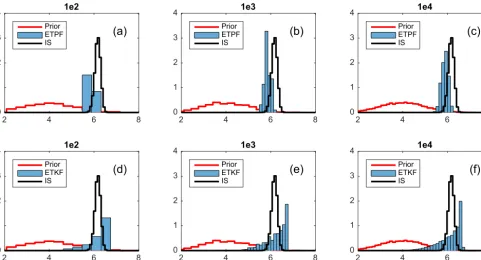
Figure 1.Probability density functions for the one-parameter nonlinear problem. Top: ETPF; bottom: ETKF.(a, d)Ensemble size 102;(b, e)ensemble size 103;(c, f)ensemble size 104. Prior is in red. The true pdf obtained by IS with ensemble size 105is in black.
3 One-parameter nonlinear problem
First we consider a one-parameter nonlinear problem from Chen and Oliver (2013). The prior distribution is a Gaussian distribution with mean 4 and variance 1. The non-linear forward model is
h(u)= 7
12u 3−7
2u 2+8u.
The true parameterutrue givesh(utrue)=48 and the obser-vation error is drawn from a Gaussian distribution with zero mean and variance 16. In Fig. 1 we plot the posterior proba-bility density functions estimated by ETPF (top) and ETKF (bottom) with ensemble sizes 102(left), 103(center), and 104 (right). The prior distribution is shown in red and the pos-terior estimated by IS with ensemble size 105 is shown in black. We can see that ETPF provides better approximation of the true probability density function, while ETKF gives a skewed posterior. It should be noted that ETKF is able to give a non-Gaussian (though wrong) posterior due to the nonlin-earity of the map between the uncertain parameters and ob-servations.
4 Single-phase Darcy flow
We consider a steady-state single-phase Darcy flow model defined over an aquifer of a 2-D physical domain D=
[0,1] × [0,1], which is given by
− ∇ ·(k(x, y)∇P (x, y))=f (x, y), (x, y)∈D P (x, y)=0, (x, y)∈∂D,
where∇ =(∂/∂x ∂/∂y)T;·denotes the dot product,P (x, y) the pressure, k(x, y) the permeability, f (x, y) the source term, which we assume to be 2π2cos(π x)cos(πy), and∂D the boundary of domain D. The forward problem of this second-order elliptical equation is to find the solution of pres-sureP (x, y)for a givenf (x, y)andk(x, y). We, however, are interested in finding permeability given noisy observa-tions of pressure at a few locaobserva-tions.
We perform numerical experiments with synthetic obser-vations, where instead of a measuring device a model is used to obtain observations. We implement a cell-centered finite difference method to discretize the domainDinton×ngrid cellsXi of size1x2 and solve the forward model with the
true parameters. Then the synthetic observations are obtained by
yobs=L(P)+η,
with an element ofL(P)being a linear functional of pressure, namely
Ll(P)=
1 2π σ2
n2
X
i=1 exp
−||Xi−rl||
2
2σ2
l∈1, . . ., Ny,
wheren=50,σ=0.01,rldenotes the location of the
obser-vation, andNy=16, which is the number of observations.
The observation locations are spread uniformly across the domainDandηdenotes the observation noise drawn from a normal distribution with zero mean and a standard deviation of 0.09. This form of the observation functional and parame-terization of the uncertain parameters given below guarantee the continuity of the forward map from the uncertain parame-ters to the observations and thus the existence of the posterior distribution as shown by Iglesias et al. (2014).
4.1 Five-parameter nonlinear problem
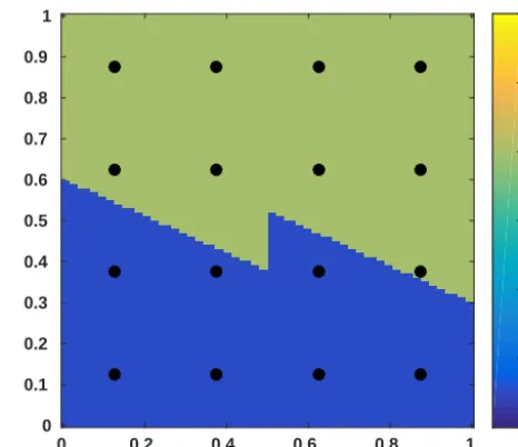
For our first numerical experiment with Darcy flow, we con-sider a low-dimensional problem where the permeability field is defined by a mere five parameters similarly to Igle-sias et al. (2014). We assume that the entire domain D= [0,1] × [0,1]is divided into two subdomainsD1andD2as shown in Fig. 2. Each subdomain ofDrepresents a layer and is assumed to have a permeability functionk(X), where an element ofXis defined byXifori=1, . . ., n2. Parametersa
andbdenote the thickness of the bottom layer on either side, which correspondingly defines the slope of the interface. A parametercdefines a vertical fault. The layer moves up or down depending onc <0 orc >0, respectively, and its loca-tion is assumed to be fixed atx=0.5.
Further, for this test case we assume piecewise constant permeability within each of the subdomains; hence,k(X)is given by
k(X)=k1δD1(X)+k2δD2(X),
wherek1andk2represent the permeability of the subdomains D1andD2, respectively, andδis the Dirac function. Then the parameters defining the permeability field for this configura-tion are
u=(a b c log(k1) log(k2))T.
We assume that the true parameters are atrue=0.6, btrue=
0.3,ctrue= −0.15,k1true=12, andk2true=5. These parame-ters are used to create synthetic observations. Figure 2 shows the true permeability, with dots representing the observation locations. Next, we assume that the five uncertain param-eters are drawn from a uniform distribution over a speci-fied interval, namely a, b∼U[0,1],c∼U[−0.5,0.5],k1∼
U[10,15], andk2∼U[4,7].
As was pointed out in Sect. 2.2, ETPF updates the pa-rameters within the original range of an initial ensemble, while ETKF does not. Therefore a change in variables has to be performed for ETKF so that the updated parameters are physically viable. In order to be consistent, we perform the change in variables for ETPF as well. As the domain D is
[0,1] × [0,1], the parametersa andb should lie within the
0 0.2 0.4 0.6 0.8 1
0 0.1 0.2 0.3 0.4 0.5 0.6 0.7 0.8 0.9 1
4 6 8 10 12 14 16
Figure 2.True permeability of the five-parameter nonlinear prob-lem with dots representing the observation locations.
interval[0,1]. To enforce this constraint, we substitutea ac-cording to
a0=log
a
1−a
, a0∈R,
and similarlybis substituted byb0. Thus the uncertain pa-rameters are nowu0=(a0b0 c log(k1) log(k2))T.
In Fig. 3 we plot probability density functions for param-etersa(panels a–d),c(panels e–h), and log(k2)(panels i–l), as the parameters b and log(k1) show similar results. The posterior obtained by IS with ensemble size 106is plotted as a black line and the true value of parameters is plotted as a black line with crosses. The posterior of ETPF is shown at the top and the posterior of ETKF at the bottom. ETPF and ETKF used 103(odd columns) and 104(even columns) en-semble members. In order to perform an objective compar-ison between the probabilities, we compute the Kullback– Leibler divergence of a posteriorπ obtained by either ETPF or ETKF and the posteriorπISobtained by IS:
DKL(πISkπ )= Nb
X
i=1
πIS(ui)log
πIS(ui)
π(ui)
(ui−ui−1), (12)
whereNb=20 is the number of bins. The Kullback–Leibler divergence for parametersa,c, and log(k2)is displayed in the titles of Fig. 3, where we observe that ETKF outperforms ETPF.
0.2 0.4 0.6 0.8 a 0 0.5 1 1.5 2 ETPF
103(0.14)
(a)
0.2 0.4 0.6 0.8
a 0 0.5 1 1.5 2
104(0.07)
(b)
0.2 0.4 0.6 0.8
a 0 0.5 1 1.5 2 ETKF 103 (0.03) (c)
0.2 0.4 0.6 0.8
a 0 0.5 1 1.5 2 104 (0.02) (d)
-0.5 0 0.5
c 0 0.5 1 1.5 ETPF 103 (0.14) (e)
-0.5 0 0.5
c
0 0.5 1 1.5
104(0.09)
(f)
-0.5 0 0.5
c 0 0.5 1 1.5 ETKF 103 (0.02) (g)
-0.5 0 0.5
c 0 0.5 1 1.5 104 (0.01) (h)
1.4 1.6 1.8
log(k2)
0 0.5 1 1.5 2 2.5 3 ETPF 103 (0.15) (i)
1.4 1.6 1.8
log(k2)
0 0.5 1 1.5 2 2.5 3 10 4(0.09) (j)
1.4 1.6 1.8
log(k2)
0 0.5 1 1.5 2 2.5 3 ETKF 103 (0.07) (k)
1.4 1.6 1.8
log(k2)
0 0.5 1 1.5 2 2.5 3 10 4 (0.05) (l)
Figure 3.Probability density functions for the parametersa(a–d),c(e–h), and log(k2)(i–l). The posterior obtained by IS with ensemble
size 106is plotted as a black line and the true values of parameters are plotted as black crosses. The posterior of ETPF is shown at the top and the posterior of ETKF at the bottom. ETPF and ETKF used 103(odd columns) and 104(even columns) ensemble members.
200 400 600 800
Ensemble size 0.2 0.3 0.4 0.5 0.6 0.7 0.8 a
(a) TruthMean IS
Mean ETPF Mean ETKF Spread ETPF Spread ETKF
200 400 600 800
Ensemble size 0.1 0.2 0.3 0.4 0.5 0.6 0.7 0.8 b (b)
200 400 600 800
Ensemble size -0.3 -0.2 -0.1 0 0.1 0.2 0.3 c (c)
200 400 600 800
Ensemble size 2.35 2.4 2.45 2.5 2.55 2.6 2.65 log ( k1 ) (d)
200 400 600 800
Ensemble size 1.45 1.5 1.55 1.6 1.65 1.7 1.75 1.8 1.85 log ( k2 ) (e) Truth Mean IS Mean ETPF Mean ETKF Spread ETPF Spread ETKF Truth Mean IS Mean ETPF Mean ETKF Spread ETPF Spread ETKF Truth Mean IS Mean ETPF Mean ETKF Spread ETPF Spread ETKF Truth Mean IS Mean ETPF Mean ETKF Spread ETPF Spread ETKF
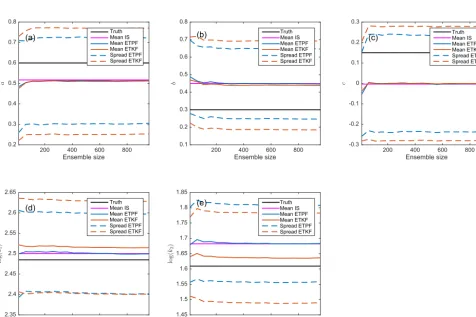
Figure 4.u¯¯aandu¯¯a± ¯uastdw.r.t. ensemble size:(a)for the parametera,(b)forb,(c)forc,(d)for log(k1), and(e)for log(k2). ETPF is
200 400 600 800
Ensemble size
-1 -0.5 0 0.5
Mi
s
fi
t
-m
i
s
a
fi
t
b
(a) ETPF
ETKF
200 400 600 800
Ensemble size
-0.3 -0.2 -0.1 0 0.1
RE
a
-R
E
b
(b) ETPF
ETKF
Figure 5.misfita,r−misfitb,r (a)and REa,r−REb,r (b)w.r.t. ensemble size. ETPF is shown in blue, ETKF in red, and the zero level in black. One circle is for one simulation.
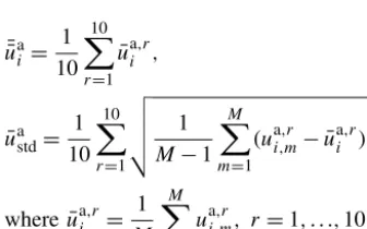
IS, the meanu¯¯a, and the spreadu¯¯a± ¯uastdof estimated param-eters averaged over 10 simulations:
¯¯
uai = 1
10 10
X
r=1
¯
uai,r,
¯
uastd= 1
10 10
X
r=1
v u u t
1 M−1
M
X
m=1
(uai,m,r − ¯uai,r)2,
whereu¯ai,r= 1
M
M
X
m=1
uai,m,r, r=1, . . .,10,
M is ensemble size, i=1, . . .,5 is the parameter index, and the superscript a is for analysis. We observe that all the methods including IS have a bias in the estimations of geometrical parameters, which is due to a small number of observations. ETPF and ETKF perform comparably in terms of mean estimation, though some are better estimated by ETKF and others are better estimated by ETPF. Comparing the error in pressure of the mean parameters we observe that the methods are equivalent (and thus not shown), which is a manifestation of the ill-posedness of the problem. In Fig. 4 we see that the spread from ETPF is smaller than from ETKF for each parameter. Both methods are slightly underdisper-sive as the spread-to-error ratio is below 1. For ensemble size 103ETKF gives(0.95 0.88 0.88 0.97 0.98)and ETPF gives (0.92 0.81 0.84 0.99 0.86) for (a b c log(k1) log(k2)). Thus ETKF gives a better ratio for all the parameters but log(k1).
We compute an average of the relative error over all pa-rameters
REa,r=1
5 5
X
i=1
| ¯uai,r−utruei |
|utruei | , r=1, . . .,10,
and the data misfit
misfita,r=(y¯a,r−yobs)TR−1(y¯a,r−yobs), r=1, . . .,10,
(13) after data assimilation. The same metrics are computed be-fore data assimilation and denoted by a superscript b. In Fig. 5a–b we plot(misfita,r−misfitb,r)and(REa,r−REb,r), respectively, for each simulationras a function of ensemble size. ETPF is shown in blue and ETKF in red. Black line is at zero level. Positive values of the differences mean an increase in either data mismatch or relative error after data assimila-tion. We observe a data misfit decrease for both ETPF and ETKF except at an ensemble size 10. RE does not always de-crease for ETPF: for some simulations ETPF is at zero level or slightly above it, while for ETKF the sole exception is at an ensemble size of 10.
4.2 High-dimensional nonlinear problem
Next, we consider a high-dimensional problem where the di-mension of the uncertain parameter isn2=2500. The do-mainDis now not divided into subdomains. However, un-like in the previous test case, here we implement a spatially varying permeability field. We assume the log permeability is generated by a random draw from a Gaussian distribution
N(log(5),C). Here5is ann2vector with all 5.Cis assumed to be an exponential correlation with an element ofCbeing Ci,j=exp(−3(|hi,j|/v)), i, j=1, . . ., n2.
Herehi,j is the distance between two spatial locations and
v is the correlation range which is taken to be 0.5. For the log permeability we use Karhunen–Loeve expansions of the form
log(kj)=log(5)+ n2
X
i=1
p
λiνi,jZi, for j=1, . . ., n2,
Gaussian distribution with zero mean and variance one. Mak-ing sure that the eigenvalues are sorted in descendMak-ing order,
Zi ∼N(0,1) produces log(k)∼N(log(5),C). The
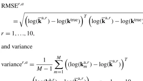
uncer-tain parameter is thusu=Zwith the dimensionn2=2500. We perform 10 different simulations based on a random draw of an initial ensemble from the prior distribution. We conduct the numerical experiments for ensemble sizes vary-ing from 10 to 103with an increment of 50. We compute the root mean square error (RMSE) of the log permeability field: RMSEr,a
= r
log(ka,r)−log(ktrue)Tlog(ka,r)−log(ktrue), r=1, . . .,10,
and variance
variancer,a= 1
M−1
M
X
m=1
(log(kam,r)−log(ka,r)
T
·log(kam,r)−log(ka,r), r=1, . . .,10. We also compute the data misfit for each simulation after data assimilation by Eq. (13). In Fig. 6 we plot mean, minimum, and maximum over 10 simulations after data assimilation for the data misfit (left), RMSE (center), and variance (right). ETPF is shown in blue and ETKF in red. We observe that ETPF is underdispersive compared to ETKF as particle filters are highly degenerative compared to Kalman filters. Misfit given by ETPF is smaller than the one given by ETKF for al-most all simulations at ensemble sizes greater than 150. The RMSE by contrast is larger.
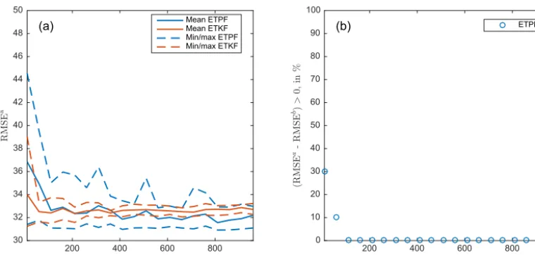
In Fig. 7a–b we plot(misfita,r−misfitb,r)and(RMSEa,r−
RMSEb,r), respectively, as a function of ensemble size for a simulationr=1, . . .,10. The superscript “b” is for the met-rics before data assimilation and the superscript “a” is for the metrics after data assimilation. ETKF always provides a de-crease in both the data misfit and RMSE except at ensemble size 10. ETPF gives a decrease in the data misfit though an in-crease in RMSE, which indicates that ETPF overfits the data. However, as the ensemble size increases, this happens less often, as can be seen in Fig. 7c, where we plot for ETPF a per-centage of simulations that result in(RMSEa−RMSEb) >0 and a linear fit as a function of ensemble size.
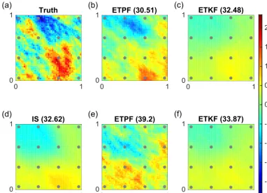
In Fig. 8 we plot log permeability fields. In Fig. 8a the true permeability is shown with dots representing the obser-vation locations, and in Fig. 8d the mean permeability field obtained by IS with ensemble size 105. The RMSE provided by IS is 32.62. In Fig. 8b–e and c–f we display mean perme-ability fields obtained with ensemble size 103by ETPF and ETKF, respectively. In Fig. 8b–c we plot the mean log per-meabilities for the smallest RMSE over simulations, which is 30.51 for ETPF and 32.48 for ETKF. In Fig. 8d–e we plot the mean log permeabilities for the largest RMSE over sim-ulations, which is 39.2 for ETPF and 33.87 for ETKF. We
observe that ETKF as well as IS provide smooth mean per-meability fields that have smaller absolute values than the true permeability. ETPF gives higher variations of the mean permeability field and is in excellent agreement with the true permeability for a good initial ensemble shown in Fig. 8b. This means that ETPF sensitivity to the initial sample is due to sampling error and that the spatial variability of ETPF is a result of sampling error. It should be noted that IS with ensemble size 103and this good initial ensemble gives the RMSE 30.51 and the same mean log permeability field as ETPF shown in Fig. 8b. However, IS does not change the parameters, only their weights, while ETPF does change the parameters. Therefore ETPF has an advantage of IS repre-senting the correct posterior but does not have its disadvan-tage of resampling lacking. In Fig. 9 we plot the variance of the permeability fields obtained with ensemble size 105 by IS (Fig. 9d), with ensemble size 103by ETPF (Fig. 9b– e) and ETKF (Fig. 9c–f). Figure 9b–c are for the smallest RMSE and Fig. 9e–f are for the largest RMSE. ETKF pro-vides smoother variance than ETPF due to smaller sampling errors.
In Fig. 10 we show the squared error(Za−Ztrue)2in blue for ETPF and in red for ETKF for three leading modesZ1 (panel a),Z2 (panel b), andZ3 (panel c), where solid line is for the median and shaded area is for the 25th and 75th percentiles over 10 simulations. We observe that in terms of the estimation of the three leading modes, ETPF outper-forms ETKF. In Fig. 11 we plot the posterior ofZ1(left),Z2 (center), andZ3 (right) obtained by IS with ensemble size 106and by ETPF (top) and ETKF (bottom) with ensemble size 104. The posterior of these modes is roughly approxi-mated by ETPF as shown in Fig. 11a–c. ETKF provides a skewed posterior of the modes shown in Fig. 11d–f, which was also observed in the one-parameter nonlinear problem; see Fig. 1f. In order to perform an objective comparison be-tween the probabilities, we compute the Kullback–Leibler di-vergence of a posteriorπ obtained by either ETPF or ETKF and the posteriorπIS obtained by IS according to Eq. (12). ETPF gives the Kullback–Leibler divergence 0.21, 0.42, and 0.6, and ETKF 0.16, 0.07, and 0.5 for the modesZ1,Z2, and
Z3, respectively. Thus ETKF gives a better approximation of the true pdf.
us-200 400 600 800 Ensemble size 0
5 10 15 20 25 30
Mi
s
fi
t
a
(a)
Mean ETPF Mean ETKF Min/max ETPF Min/max ETKF
200 400 600 800
Ensemble size 30
32 34 36 38 40 42 44 46 48 50
RMSE
a
(b) Mean ETPF
Mean ETKF Min/max ETPF Min/max ETKF
200 400 600 800
Ensemble size 0
5 10 15 20 25 30 35 40 45 50
Var
i
a
n
c
e
a
(c)
Mean ETPF Mean ETKF Min/max ETPF Min/max ETKF
Figure 6.Mean, minimum, and maximum over 10 simulations after data assimilation for the data misfit(a), RMSE(b), and variance(c). ETPF is shown in blue and ETKF in red.
200 400 600 800
Ensemble size -10
-5 0 5 10 15 20
RMSE
a
-R
M
S
E
b
(b)
ETPF ETKF
200 400 600 800
Ensemble size -20
-15 -10 -5 0 5 10
Mi
s
fi
t
-m
i
s
a
fi
t
b
(a)
ETPF ETKF
200 400 600 800
Ensemble size 0
10 20 30 40 50 60 70 80 90 100
(RMSE
a
-R
M
S
E
b)
>
0,
in
%
(c) ETPF
Linear fit
Figure 7.misfita,r−misfitb,r (a)and RMSEa,r−RMSEb,r(b)w.r.t. ensemble size. ETPF is shown in blue, ETKF in red and zero level in black. One circle is for one simulation. For ETPF % of simulations that result in(RMSEa−RMSEb) >0 and a linear fit as a function of ensemble size are shown in(c).
ing the full Karhunen–Loeve expansions, we observe that the maximum RMSE over simulations decreased substantially, while the minimum RMSE only slightly increased. ETKF gives RMSE at the best sample 32.27 and the worst sample 33.23. (Compare to 32.48 and 33.9 using the full Karhunen– Loeve expansions.) Thus ETKF slightly decreases both max-imum and minmax-imum RMSE over simulations. ETPF is more affected by sampling noise at small scales, so using a trun-cated representation of the fields significantly improves the results for ETPF. ETKF filters out the small scales that are not observed and thus is less affected by the truncation.
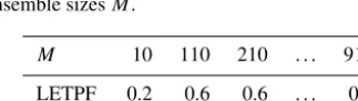
Next we apply LETPF and LETKF. The optimal localiza-tion radius between 0.2 and 1.2 was obtained in terms of the smallest RMSE and shown in Table 1. It should be noted that a smaller localization radius for LETPF than for LETKF was
Table 1.Optimal localization radius for LETPF and LETKF at dif-ferent ensemble sizesM.
M 10 110 210 . . . 910
LETPF 0.2 0.6 0.6 . . . 0.6 LETKF 0.2 1.2 1.2 . . . 1.2
0 1 0
1 Truth
(a)
0 1
0
1 ETPF (30.51)
(b)
0 1
0
1 ETKF (32.48)
(c)
0 1
0
1 IS (32.62)
(d)
0 1
0
1 ETPF (39.2)
(e)
0 1
0
1 ETKF (33.87)
(f)
-2 -1.5 -1 -0.5 0 0.5 1 1.5 2
Figure 8.Log permeability field with dots representing the observation locations. Truth is shown in (a)and mean obtained by IS with ensemble size 105in(d). Mean obtained with ensemble size 103by ETPF shown in(b)–(e)and by ETKF in(c)–(f), where(b)–(c)are at the smallest RMSE and(e)–(f)are at the largest RMSE over simulations. The corresponding RMSE is given in parentheses.
0 1
0
1 ETPF
(b)
0 1
0
1 ETKF
(c)
0 1
0
1 IS
(d)
0 1
0
1 ETPF
(e)
0 1
0
1 ETKF
(f)
0.2 0.4 0.6 0.8 1 1.2 1.4 1.6 1.8
200 400 600 800 Ensemble size 0
0.05 0.1 0.15 0.2 0.25
Z1 (a)
IS ETPF ETKF
200 400 600 800
Ensemble size 0
0.2 0.4 0.6 0.8 1 1.2
Z2 (b)
IS ETPF ETKF
200 400 600 800
Ensemble size 0
0.2 0.4 0.6 0.8 1 1.2 1.4
Z3 (c)
IS ETPF ETKF
Figure 10.Squared error between the true and mean estimated modes forZ1(a),Z2(b), andZ3(c)w.r.t. ensemble size. ETPF is shown in blue and ETKF in red, with solid lines for median and shaded area for the 25th and 75th percentiles over 10 simulations. IS with ensemble size 105is in black.
-2 -1 0 1
Z1
0 0.5 1 1.5 2 2.5
ETPF
104(0.21)
(a)
-2 -1 0 1
Z2
0 0.5 1 1.5 2 2.5
ETPF
104(0.42)
(b)
-3 -2 -1 0 1
Z3
0 0.5 1 1.5 2 2.5
ETPF
104(0.6)
(c)
-2 -1 0 1
Z1
0 0.5 1 1.5 2 2.5
ETKF
104(0.16)
(d)
-2 -1 0 1
Z2
0 0.5 1 1.5 2 2.5
ETKF
104(0.07)
(e)
-3 -2 -1 0 1
Z3
0 0.5 1 1.5 2 2.5
ETKF
104(0.49)
(f)
Figure 11.The posterior probability density function of parametersZ1(a, d),Z2(b, e), andZ3(c, f). The posterior obtained by IS with
ensemble size 106is plotted as a black line and the true parameter as a black cross. The posterior of ETPF is shown at the top and the posterior of ETKF at the bottom. Both ETPF and ETKF used 104ensemble members. The Kullback–Leibler divergence is in parentheses.
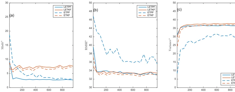
At small ensemble sizes both LETKF and LETPF give smaller misfit, smaller RMSE but larger variance than ETKF and ETPF. For large ensembles LETKF performs worse than ETKF, which is due to the imposed range on localization ra-dius, meaning that 1.2 is not optimal. Comparing the per-formance of LETPF to (L)ETKF we observe that at small ensemble sizes LETKF still outperforms ETPF, but at large ensemble sizes LETPF performs now comparably to ETKF. Moreover, LETPF overfits the data less often than ETPF: 40 % against 90 % for ensemble size 10 % and 0 % against non-zero % for ensemble sizes greater than 150 (not shown).
In Figs. 15–16 we plot mean and variance of the log per-meability field at ensemble size 103 for ETPF (panels b– e) and ETKF (panels c–f) with localization at the smallest RMSE (panels b–c) and largest RMSE (panels e–f) over sim-ulations, which are 32.29 and 34.08 for ETPF and 32.92 and 34.09 for ETKF, respectively. We observe that localization decreases the sampling noise and the spatial variability of the mean field obtained by ETPF at ensemble size 103resembles IS at ensemble size 105. The variance obtained by ETPF with localization shown in Fig. 16b–e has also improved.
200 400 600 800 Ensemble size
30 32 34 36 38 40 42 44 46 48 50
RMSE
a
(a) Mean ETPFMean ETKF
Min/max ETPF Min/max ETKF
200 400 600 800
Ensemble size 0
10 20 30 40 50 60 70 80 90 100
(RMSE
a-R
M
S
E
b)
>
0,
in
%
(b) ETPF
Figure 12.Using only three leading modes in the KL expansion.(a)RMSE after data assimilation w.r.t. ensemble size with mean, minimum and maximum over 10 simulations for ETPF shown in blue and ETKF in red.(b)% of simulations that result in(RMSEa−RMSEb) >0 for ETPF.
0 1
0
1 Truth
(a)
0 1
0
1 ETPF (31.1) (b)
0 1
0
1 ETKF (32.27) (c)
0 1
0
1 IS (31.39) (d)
0 1
0
1 ETPF (32.98) (e)
0 1
0
1 ETKF (33.23) (f)
-2 -1.5 -1 -0.5 0 0.5 1 1.5 2
Figure 13.Same as Fig. 8 but using only three leading modes in the KL expansion.
Leibler divergence for the leading mode is 0.73 (compared to 0.21 without localization), and for the second and third modes it is 0.2 and 0.18, respectively (compared to 0.42 and 0.6 without localization). Variance of the posteriors is larger when localization is applied for both methods. The localized weights given by Eq. (10) vary less than the non-localized weights given by Eq. (3). Therefore the localized pdf is less noisy than the non-localized pdf. However, localization ap-plied in the form of the Karhunen–Loeve expansion given by Eq. (14) does not retain the imposed bounds on the modes
Z, as we need to invert a matrix product of eigenvalue and eigenvector matrices to obtain the modes. Moreover, unlike ETKF, LETPF does not converge to ETPF as the localization radius goes to infinity due to the transport problem being uni-variate for LETPF and multiuni-variate for ETPF.
5 Conclusions
param-200 400 600 800
Ensemble size
0 5 10 15 20 25 30
Mi
sfi
t
a
(a)
LETPF LETKF ETPF ETKF
200 400 600 800
Ensemble size
30 32 34 36 38 40 42 44 46 48 50
RMSE
a
(b) LETPFLETKF
ETPF ETKF
200 400 600 800
Ensemble size
0 5 10 15 20 25 30 35 40 45 50
Va
r
i
a
n
c
e
a
(c)
LETPF LETKF ETPF ETKF
Figure 14.Mean over 10 simulations after data assimilation for the data misfit(a), RMSE(b), and variance(c). LETPF is shown in solid blue and LETKF in solid red. ETPF is shown in dashed blue and ETKF in dashed red.
0 1
0
1 Truth
(a)
0 1
0
1 LETPF (32.29)
(b)
0 1
0
1 LETKF (32.92)
(c)
0 1
0
1 IS (32.62)
(d)
0 1
0
1 LETPF (34.08)
(e)
0 1
0
1 LETKF (34.09)
(f)
-2 -1.5 -1 -0.5 0 0.5 1 1.5 2
Figure 15.Same as Fig. 8 but with localization.
eters and states. They, however, also remain computationally expensive. Ensemble Kalman filters (ETKFs) provide com-putationally affordable approximations but rely on the as-sumptions of Gaussian probabilities. For nonlinear models, even if the prior is Gaussian, the posterior is not Gaussian anymore. Particle filtering on the other hand does not have
0 1 0
1 LETPF
(b)
0 1
0
1 LETKF
(c)
0 1
0
1 IS
(d)
0 1
0
1 LETPF
(e)
0 1
0
1 LETKF
(f)
0.3 0.35 0.4 0.45 0.5 0.55 0.6 0.65 0.7 0.75 0.8
Figure 16.Same as Fig. 9 but with localization.
ETPF certainly outperforms ETKF for a one-parameter nonlinear test case by giving a better posterior estimation. For the five-parameter test case, the mean estimations tained by ETPF are not consistently better than the ones ob-tained by ETKF, and the spread is smaller. The Kullback– Leibler divergence from ETKF is smaller than from ETPF for all the parameters. When the number of uncertain param-eters is large (2500), a decrease in degrees of freedom is es-sential. This is performed by localization. At large ensemble sizes LETPF performs as well as LETKF, while at small en-semble sizes LETKF still outperforms LETPF. Even though LETPF overfits the data less often than ETPF, localization destroys the property of ETPF to retain the imposed bounds. This deteriorates a posterior estimation of the leading mode. Another plausible drawback of localization is an assumption of observations being local, which might not be the case for inverse modeling. An alternative approach to improve ETPF performance is instead by applying localization to use only leading modes in the approximation of log permeability, as they are better estimated by the method. However, one needs to know at which mode to truncate, and this is highly depen-dent on the covariance matrix of log permeability.
To conclude, we believe that ETPF is promising for in-verse modeling. However, more theoretical studies have to be performed for ETPF before it is considered for realistic applications. Plausible issues related to realistic application are numerous accurate observations, time dependency of an underlying model, and a flow being multiphase, for example.
Data availability. Data and MATLAB codes for generating the
plots are available in Dubinkina and Ruchi (2018).
Author contributions. All authors contributed equally to this work.
Competing interests. The authors declare that they have no conflict
of interest.
Acknowledgements. This work is part of the research programme
Shell-NWO/FOM Computational Sciences for Energy Research (CSER) with project number 14CSER007 which is partly financed by the Netherlands Organization for Scientific Research (NWO).
Edited by: Takemasa Miyoshi Reviewed by: two anonymous referees
References
Aanonsen, S. I., Nævdal, G., Oliver, D. S., Reynolds, A. C., and Vallès, B.: The ensemble Kalman filter in reservoir engineering – a review, SPE Journal, 14, 393–412, 2009.
Chen, Y. and Oliver, D. S.: Levenberg–Marquardt forms of the it-erative ensemble smoother for efficient history matching and un-certainty quantification, Computat. Geosci., 17, 689–703, 2013. Cheng, Y. and Reich, S.: Data assimilation: a dynamical system
per-spective, Frontiers in Applied Dynamical Systems: Reviews and Tutorials, 2, 75–118, 2015.
Doucet, A., de Freitas, N., and Gordon, N.: Sequential Monte-Carlo Methods in Practice, Springer-Verlag, New York, 2001. Dovera, L. and Della Rossa, E.: Multimodal ensemble Kalman
fil-tering using Gaussian mixture models, Computat. Geosci., 15, 307–323, 2011.
Dubinkina, S. and Ruchi, S.: Data underlying the paper: Appli-cation of ensemble transform data assimilation methods for parameter estimation in reservoir modeling, 4TU, Centre for Research Data, Dataset, https://doi.org/10.4121/uuid:2d0018ea-fecc-4d19-8532-5a718c9f28ca, 2018.
Evensen, G.: Data assimilation: the ensemble Kalman filter, Springer Science & Business Media, Berlin, Germany, 2009. Gaspari, G. and Cohn, S. E.: Construction of correlation functions
in two and three dimensions, Q. J. Roy. Meteor. Soc., 125, 723– 757, 1999.
Plaza, D. A., De Keyser, R., De Lannoy, G. J. M., Giustarini, L., Matgen, P., and Pauwels, V. R. N.: The importance of parame-ter resampling for soil moisture data assimilation into hydrologic models using the particle filter, Hydrol. Earth Syst. Sci., 16, 375– 390, https://doi.org/10.5194/hess-16-375-2012, 2012.
Hunt, B., Kostelich, E., and Szunyogh, I.: Efficient data assimilation for spatialtemporal chaos: A local ensemble transform Kalman filter, Physica D, 230, 112–137, 2007.
Iglesias, M. A., Lin, K., and Stuart, A. M.: Well-posed Bayesian ge-ometric Inverse Probl. arising in subsurface flow, Inverse Probl., 30, 114001, https://doi.org/10.1088/0266-5611/30/11/114001, 2014.
Moradkhani, H., Sorooshian, S., Gupta, H. V., and Houser, P. R.: Dual state–parameter estimation of hydrological models using ensemble Kalman filter, Adv. Water Resour., 28, 135–147, 2005.
Oliver, D. S. and Chen, Y.: Recent progress on reservoir history matching: a review, Computat. Geosci., 15, 185–221, 2011. Oliver, D. S., Cunha, L. B., and Reynolds, A. C.: Markov chain
Monte Carlo methods for conditioning a permeability field to pressure data, Math. Geol., 29, 61–91, 1997.
Oliver, D. S., Reynolds, A. C., and Liu, N.: Inverse theory for petroleum reservoir characterization and history matching, Cam-bridge University Press, CamCam-bridge, UK, 2008.
Pele, O. and Werman, M.: Fast and robust earth mover’s distances, in: Computer vision, 2009 IEEE 12th inter-national conference on, IEEE, Kyoto, Japan, 460–467, https://doi.org/10.1109/ICCV.2009.5459199, 2009.
Penny, S. G. and Miyoshi, T.: A local particle filter for high-dimensional geophysical systems, Nonlin. Processes Geophys., 23, 391–405, https://doi.org/10.5194/npg-23-391-2016, 2016. Poterjoy, J.: A localized particle filter for high-dimensional
nonlin-ear systems, Mon. Weather Rev., 144, 59–76, 2016.
Reich, S. and Cotter, C.: Probabilistic forecasting and Bayesian data assimilation, Cambridge University Press, Cambridge, UK, 2015.
Reynolds, A. C., He, N., Chu, L., and Oliver, D. S.: Reparameteriza-tion techniques for generating reservoir descripReparameteriza-tions condiReparameteriza-tioned to variograms and well-test pressure data, SPE Journal, 1, 413– 426, 1996.
Vefring, E. H., Nygaard, G. H., Lorentzen, R. J., Naevdal, G., and Fjelde, K. K.: Reservoir characterization during underbalanced drilling (ubd): methodology and active tests, SPE Journal, 11, 181–192, 2006.