www.ocean-sci.net/2/27/2006/
© Author(s) 2006. This work is licensed under a Creative Commons License.
Ocean Science
The circulation of the Persian Gulf: a numerical study
J. K¨ampf1and M. Sadrinasab2
1School of Chemistry, Physics and Earth Sciences, Flinders Research Centre for Coast and Catchment Environments, Flinders University, Adelaide, Australia
2Khorramshahr University of Nautical Sciences & Technology, Khorramshahr, Iran Received: 4 March 2005 – Published in Ocean Sci. Discuss.: 12 May 2005 Revised: 20 April 2006 – Accepted: 30 May 2006 – Published: 5 July 2006
Abstract. We employ a three-dimensional hydrodynamic model (COHERENS) in a fully prognostic mode to study the circulation and water mass properties of the Persian Gulf – a large inverse estuary. Our findings, which are in good agree-ment with observational evidence, suggest that the Persian Gulf experiences a distinct seasonal cycle in which a gulf-wide cyclonic overturning circulation establishes in spring and summer, but this disintegrates into mesoscale eddies in autumn and winter. Establishment of the gulf-wide cir-culation coincides with establishment of thermal stratifica-tion and strengthening of the baroclinic exchange circula-tion through the Strait of Hormuz. Winter cooling of ex-treme saline (>45) water in shallow regions along the coast of United Arab Emirates is a major driver of this baroclinic circulation.
1 Introduction
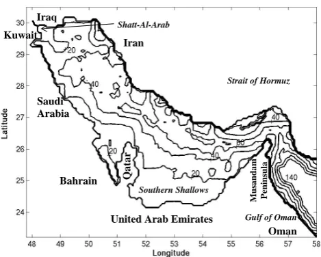
The Persian Gulf, referred to in some local countries as the Arabian Gulf, is an important military, economic and politi-cal region owing to its oil and gas resources and is one of the busiest waterways in the world. Countries bordering the Per-sian Gulf are the United Arab Emirates, Saudi Arabia, Qatar, Bahrain, Kuwait and Iraq on one side and Iran on the other side (Fig. 1).
The Persian Gulf is∼990 km long and has a maximum width of 370 km. The average depth of the Gulf is 36 m. The Persian Gulf occupies a surface area of∼239 000 km2 (Emery, 1956). Extensive shallow regions,<20 m deep, are found along the coast of United Arab Emirates (hereafter re-ferred to as Southern Shallows), around Bahrain, and at the head of the Gulf. Deeper portions,>40 m deep, are found along the Iranian coast continuing into the Strait of Hormuz,
Correspondence to: J. K¨ampf
which has a width of∼56 km and connects the Persian Gulf via the Gulf of Oman with the northern Indian Ocean.
Tectonic driven subsidence deepened the seafloor of the Strait on its southern side (200–300 m depths are seen in some localised seafloor depressions) and produced a 70– 95 m deep trough along the Iranian side of the eastern part of the Gulf. A southward widening channel leads from the Strait south across a series of sills (water depth of∼110 m) and shallow basins to the shelf edge (Seibold and Ulrich, 1970). The narrow Strait of Hormuz restricts water exchange between the Persian Gulf with the northern Indian Ocean.
The Persian Gulf is a semi-enclosed, marginal sea that is exposed to arid, sub-tropical climate. It is located between latitudes 24◦–30◦N, and is surrounded by most of the Earth’s deserts. The most known weather phenomenon in the Persian Gulf is the Shamal, a northwesterly wind which occurs year round (Perrone, 1981). In winter, the Shamal is of intermit-tent nature associated with the passage of synoptic weather systems, but it seldom exceeds a speed of 10 m/s. The sum-mer Shamal is of continuous nature from early June through to July. Seasonal variations of the Shamal are associated with the relative strengths of the Indian and Arabian thermal lows (Emery, 1956).
The Gulf experiences evaporation rates of ∼2 m/yr (per unit surface area) (Privett, 1959; Hastenrath and Lamb, 1979; Meshal and Hassan, 1986; Ahmad and Sultan, 1990) that exceed by far the net freshwater input by precipitation (∼0.15 m/yr) (Johns et al., 2003) and river discharge. The major river source in the Persian Gulf is the Shatt-Al-Arab (called Arvand Roud by some countries), being located at the head of the Gulf and being fed by the Euphrates, Tigris and Karun rivers.
Previous estimates of the annual-mean discharge of the Shatt-Al-Arab vary from 35 km3/yr (Saad, 1978; Johns et al., 2003), being equivalent to 0.15 m/yr when being evenly distributed over the surface of the gulf, to ∼45 km3/yr (0.19 m/yr) (Wright, 1974; Reynolds, 1992). These values are likely an overestimate of current river discharge that has
28 J. K¨ampf and M. Sadrinasab: The circulation of the Persian Gulf
27 Figure 1. Bathymetry (CI = 20 m) used in this study.
Iran Iraq
Saudi Arabia Kuwait
Qatar
United Arab Emirates
Oman
Strait of Hormuz
Gulf of Oman
Bahrain
Southern Shallows
Mus
a
nd
am
Peninsula
Shatt-Al-Arab
Fig. 1. Bathymetry (CI=20 m) used in this study.
been reduced to an unknown extent by dam constructions, such as the Atat¨urk dam built in the Euphrates by Turkey in 1990 and other dams and reservoirs built by Iran, Iraq, and Syria.
The U.S. Naval Oceanographic Office (Alessi et al., 1999) has archived historical temperature-salinity observations in the Persian Gulf. This data consists of a number of 1597 temperature-salinity profiles, including Mt. Mitchell data (Reynolds, 1993), and spans observations over 73 years from 1923 to 1996. The Mt. Mitchell expedition comprised 500 CTD casts taken in the Persian Gulf, the Strait of Hormuz and the Gulf of Oman over a period of 3.5 months (26 February– 12 June 1992) (Reynolds, 1993). No autumn field data are available for the Gulf. Data coverage in the Southern Shal-lows and around Bahrain is poor. Alessi et al. (1999) present this data in the form of temperature-salinity-season diagrams that we use for model validation and interpretation of find-ings. Swift and Bower (2003) (henceforth SB2003) analyse and discuss this data in detail.
Owing to excess evaporation, the Persian Gulf exhibits a reverse estuarine circulation in which, due to geostrophy, the dense bottom outflow follows the coastline of United Arab Emirates, whereas inflow of Indian Ocean Surface Water (IOSW) follows the Iranian coastline (Sugden, 1963; Hunter, 1982; Chao et al., 1992; Reynolds, 1993; Johns et al., 2003; SB2003). Reynolds (1993) and others (e.g. Hunter, 1983) proposed that the densest water driving this bottom outflow formed in the Southern Shallows. Contrary to this, on the basis of an axial transect, SB2003 argued that the densest water formed near the head of the Gulf and suggested that water masses of the Southern Shallows were too warm in winter and thus not dense enough to drive the bottom outflow. This conclusion, however, might be biased by the location of this transect which does not include the Southern Shallows (see Fig. 7a in SB2003). Winter transects reaching into the
Southern Shallows (see Figs. 8a–b in SB2003), however, re-veal high densities (>1030 kg m−3)in this region exceeding values observed near the head. Also indicated are local injec-tions of this dense water into the main outflow, seen as a local salinity and density maximum in the axial section in vicinity of the Southern Shallows (see Fig. 7a in SB2003). Therefore, the authors deem the conclusion of SB2003, stating that the densest water forms at the Gulf’s head, elusory.
Direct observations of the circulation within the Persian Gulf are scarce. Ship-drift records indicate northwestward flow of speeds>10 cm/s along the Iranian coast to a change in trend of the coast near 51.5◦E and southwestward flow in the southern Gulf away from Iran (Hunter, 1983; Chao et al., 1992). Findings from vector-averaging current meters and drifter buoys, deployed during the Mt. Mitchell cruises, par-tially agree with the historic ship drift data. There are occa-sions of disagreement where the northwestward coastal flow weakened to speeds <3 cm/s near the surface, presumably due to the presence of strong north-westerly winds during the time of measurement (SB2003).
The salinity distribution in the Persian Gulf experiences significant seasonal variations. For unknown reasons, the inflow of IOSW strengthens in late spring and summer and moves further up the Iranian coastline and closer to the coast of United Arab Emirates (Reynolds, 1993; SB2003). This leads to formation of a pronounced summer salinity front in the Persian Gulf with the 39-salinity contour following largely the 40-m depth contour (see Reynolds, 1993). Salin-ity varies across the front by 2 over a distance of 50–100 km. SB2003 suggested that this front represent a region of mix-ing between water masses and not a boundary between flows moving in different directions. In winter, the front retreats toward the Strait of Hormuz by∼200 km (see SB2003). As a result of this, surface Gulf waters are saltier in winter than in summer, which has puzzled physical oceanographers for many decades. Schott (1908) attributed the difference to changing river fluxes. Emery (1956) attributed this feature to seasonal changes in evaporation rates. Chao et al. (1992) suggested that wind stress hindered the inflow of IOSW into the Persian Gulf during winter. On the basis of initial find-ings of Johns and Olson (1998), SB2003 argued that the dense outflow be steady and therefore be not correlated to variations of the influx of IOSW. Instead of this, they pro-posed that variable influx of IOSW be driven by seasonally variable evaporative lowering of sea surface height. We were not fully satisfied with either of these interpretations as these did not account for mixing processes in the water column that might remove surface salinity extremes.
outflow, carrying a layer-averaged salinity of 39.5, varies by ±20% seasonally and appears to be strongest in late spring and summer (see Johns et al., 2003) in conjunction with peak inflow IOSW into the Gulf. Thus, there appears to be a cor-relation between the strength of the bottom outflow and that of the IOSW inflow, which conflicts with SB2003, who claim that the magnitude of the bottom outflow should peak in win-ter.
Observational evidence suggests the existence of a coastal upwelling jet that flows southeastward along the northern Ira-nian coast to at least 28◦N (see Reynolds, 1993). There is sedimentological evidence that this current is a long-term feature that significantly affects sediment transport in the northern Gulf (Uchupi et al., 1996).
Tides in the Persian Gulf are complex and the dominant pattern varies from being primarily semi-diurnal to diurnal (Reynolds, 1993). Major semi-diurnal and diurnal tidal con-stituents in the Persian Gulf are M2, S2, K1, and O1(Najafi, 1997). Semi-diurnal constituents have two amphidromic points that sit in the north-western and southern ends of the Gulf, respectively. The diurnal constituents have a single amphidromic point in the centre of the Gulf near Bahrain (Hunter, 1982). Tidal hydrodynamic simulations (e.g. Najafi, 1997) predict tidal flows of∼0.9 m/s near the Strait of Hor-muz and at the head of the Gulf, and 0.3–0.6 m/s elsewhere in the Gulf.
Chao et al. (1992) studied the circulation of the Persian Gulf with a three-dimensional hydrodynamic model under realistic meteorologic forcing. Model predictions indicate that inflow through the Strait peaks at 0.17 Sv in March and decrease to 0.03 Sv in August–September, the latter being far too weak as compared with ADCP data (Johns et al., 2003). Chao et al. (2003) were able to simulate the cy-clonic overturning circulation in the Gulf, but their simula-tions had some shortcomings. Firstly, the lateral grid spacing used (∼20 km) did not resolve the internal deformation ra-dius (∼20 km), so that mesoscale instabilities could not ade-quate be described. Secondly, the total simulation time was limited to 2 years, which may not have been sufficiently long for the model to approach of steady seasonal cycle.
This paper focuses on several aspects of the circulation in the Persian Gulf that have not been comprehensively ad-dressed before. Where are the source regions of dense water formation that drive the outflow through the Strait of Hor-muz? Which factors control the seasonally variable exchange circulation through the Strait? Which processes make the Persian Gulf saltier in winter compared to summer? What are the patterns of circulation and water mass properties in autumn where field data are lacking?
To answer these questions, we employ an eddy-resolving, three-dimensional numerical model under realistic climato-logic forcing and accurate bottom topography. This model differs from the model application by Chao et al. (1992) in that the spatial grid spacing is much finer (∼7 km), which improves the spatial resolution of mesoscale instabilities, and
that total simulation times are much longer (20 years), so that the last years of prediction are uninfluenced by initial condi-tions. It is noticeable that Sadrinasab and K¨ampf (2004) em-ployed a similar model configuration to derive flushing times in the Persian Gulf.
This paper is organised as follows. Section 2 describes the model and the design of experiments. Section 3 discusses the model findings. Section 4 presents conclusions and recom-mendations for future studies.
2 Model
2.1 Governing equations
We employ the hydrodynamic part of COHERENS (COu-pled Hydrodynamical Ecological model for REgioNal Shelf seas) (Luyten et al., 1999) which is based on a bottom-following vertical sigma coordinate. The model is run in a fully prognostic mode with Cartesian lateral coordinates on the f plane, using a geographical latitude of 27◦N. The model is based on hydrostatic versions of the Navier-Stokes equations that embrace conservation equations for momen-tum, volume, heat and salt. The Boussinesq approximation is included in the horizontal momentum equations. The sea surface can move freely; that is, barotropic shallow water motions such as those associated with surface gravity waves are included. The equation of state as defined by the Joint Panel on Oceanographic Tables and Standards (UNESCO, 1981) has been used, wherein pressure effects on density are ignored. See Luyten et al. (1999) for details on hydrody-namic equations and their formulation in sigma coordinates. 2.2 Model domain and grid resolution
We employ 5 sigma levels and Cartesian lateral grid spac-ings of 1x=7.4 km (east-west direction) and 1y=6.6 km (north-south direction). Bathymetry and coastline locations are based on ETOPO-2 data that has been interpolated and slightly smoothed onto a 4-min grid (see Fig. 1). This re-moved local topographic irregularities, often a cause for nu-merical instabilities, in particular in the Strait of Hormuz. Minimum water depth is chosen at 5 m and maximum water depth is restricted to 140 m, which applies only to the Gulf of Oman and has no significant impact on the results. Note that restriction to 5 sigma levels is a compromise to max-imise model efficiency with relatively fine lateral resolution and long simulation times (∼20 years). Shorter simulations with 10 sigma levels yielded similar results (not shown). 2.3 Initial and boundary conditions
The model is initialised in winter when vertical stratifica-tion is weak throughout the Gulf using uniform tempera-ture and salinity fields with values of 20◦C and 38, respec-tively, which is reasonably close to observational evidence
30 J. K¨ampf and M. Sadrinasab: The circulation of the Persian Gulf
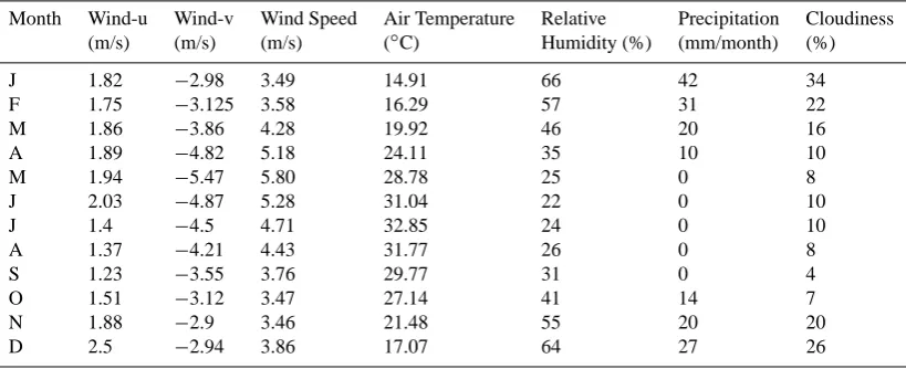
Table 1. Climatological data used in model simulations.
Month Wind-u Wind-v Wind Speed Air Temperature Relative Precipitation Cloudiness (m/s) (m/s) (m/s) (◦C) Humidity (%) (mm/month) (%)
J 1.82 −2.98 3.49 14.91 66 42 34
F 1.75 −3.125 3.58 16.29 57 31 22
M 1.86 −3.86 4.28 19.92 46 20 16
A 1.89 −4.82 5.18 24.11 35 10 10
M 1.94 −5.47 5.80 28.78 25 0 8
J 2.03 −4.87 5.28 31.04 22 0 10
J 1.4 −4.5 4.71 32.85 24 0 10
A 1.37 −4.21 4.43 31.77 26 0 8
S 1.23 −3.55 3.76 29.77 31 0 4
O 1.51 −3.12 3.47 27.14 41 14 7
N 1.88 −2.9 3.46 21.48 55 20 20
D 2.5 −2.94 3.86 17.07 64 27 26
(see Alessi et al., 1999). The model is forced by climatologic monthly mean atmospheric forcing (wind speed, air temper-ature, humidity, cloud cover and precipitation) at 10-m ref-erence height above ground derived from 54 years (1948– 2002) of NOAA data (Table 1).
The shortwave radiative flux is calculated on an hourly ba-sis to resolve its diurnal variation. Atmospheric conditions are assumed to be uniform in space but variable in time. A quadratic bulk formula is used to calculate surface frictional stresses with a wind-dependant formulation of the drag coef-ficient proposed by Geernaert et al. (1986); that is,
CDs =10−3(0.43+0.097|U10|) (1) where U10 is the wind speed at 10 m above ground. Con-ventional bulk formulae are used to derive local evaporation rate and residual surface heat flux owing to shortwave and longwave radiation plus sensible and latent heat fluxes. Tur-bulent exchange coefficients for latent and sensible heat are assumed to be functions of both wind speed and air-sea tem-perature differences (see Luyten et al., 1999). This implies that stability of the atmospheric boundary layer enters the bulk formulae as variable Dalton and Stanton numbers. For simplicity, we assume that solar radiation is absorbed within the upper layer of the model. The surface salt (freshwater) flux is a function of sea surface salinity, and the difference between evaporation and precipitation rates.
Coastlines and seabed are impermeable boundaries where normal fluxes of heat and salt vanish. A quadratic bottom-drag formula is used in which the bottom-drag coefficient is a func-tion of the roughness length according to
CDb =nk/lnzrz o
o2
, (2)
wherezr is a reference height taken at the grid centre of the bottom cell,κ=0.4 is van Karman’s constant, andzo repre-sents the bottom roughness length. The latter parameter has
been chosen atzo=0.003 m following a number of tidal sim-ulations. This gave reasonable agreement with previous tidal studies (e.g. Najafi, 1997).
River discharge is implemented in the model by means of inflow of a low-salinity (salinity is 20) surface layer of 1.5 m in thickness and 700 m in width. Riverine inflow is assumed to vary in a sinusoidal fashion with minimum val-ues of 350 m3/s in October and a maximum of 650 m3/s in April. This gives an annual-mean river discharge of 500 m3/s (15.8 km3/yr), which we deem a realistic estimate of current discharge rates. Tidal influences on this discharge are ig-nored. River temperatures are assumed to vary between min-imum values of 16◦C in December and peak values of 32◦C in July.
Amplitudes and phases of the four major tidal constituents, M2, S2, O1, and K1, are prescribed as constant values along the eastern open-ocean boundary (Table 2). Co-amplitudes and co-phases (not shown) predicted for each of the above tidal constituents in the Persian Gulf differ by less than 10% compared with previous simulations (Landner et al., 1982; Le-Provost, 1984; El-Shabh and Murty, 1988; Bashir et al., 1989; Protor et al., 1994; Najafi, 1997). In the context of this work, we take this as an accurately enough representation of tides in the Persian Gulf. The reference sea level along the open-ocean boundary is kept constant over time.
Table 2. Tidal amplitudes and phases prescribed at the eastern boundary.
Tidal Constituent Period (h) Amplitude (m) Phase (deg)
Principal lunar semidiurnal M2 12.42 1.1 214.980 Principal lunar diurnal O1 25.82 0.6326 192.200 Principal solar semidiurnal S2 12.00 0.4416 248.900 Lunisolar diurnal K1 23.93 0.3378 289.300
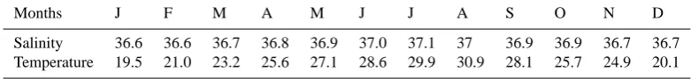
Table 3. Monthly mean upper-ocean salinity and temperature (◦C) values prescribed at the eastern boundary.
Months J F M A M J J A S O N D
Salinity 36.6 36.6 36.7 36.8 36.9 37.0 37.1 37 36.9 36.9 36.7 36.7 Temperature 19.5 21.0 23.2 25.6 27.1 28.6 29.9 30.9 28.1 25.7 24.9 20.1
slowly adjust the boundary profiles from initially uniform values to real values over the first simulation year.
2.4 Turbulence closure
Turbulent viscosity is assumed to equal turbulent diffusivity. The horizontal turbulent exchange coefficient,Ah, is taken proportional to the product of lateral grid spacings,1x and
1y, and the sheared velocities, in analogy with Smagorin-sky’s (1963) parameterisation; that is,
Ah=c1x1yDT , (3a)
where
D2T= ∂u∂x2+ ∂v∂y2+0.5 ∂u∂y+∂v∂x2, (3b) where uandv are zonal and meridional flow components, and the parameterchas been chosen atc=0.2 (Oey and Chen 1992). In our simulations, horizontal turbulent exchange co-efficient attains typical values of 15 m2/s with peak local val-ues in the Strait of Hormuz of∼150 m2/s. Vertical turbulence is parameterised by a level 2.5 turbulence closure of Mel-lor and Yamada (1982) with the modifications introduced by Galperin et al. (1988). This gave reasonably accurate predic-tions of the seasonal cycle of vertical stratificapredic-tions of tem-perature and salinity in the Persian Gulf (see Sect. 3). 2.5 Numerical implementations
The model equations are discretised on an Arakawa C-grid (Arakawa and Suarez, 1983). A mode-splitting technique is employed to maximise model performance. A predictor-corrector method is used to solve the horizontal momentum equations. This satisfies the requirement that, when using a mode-splitting technique of solution, the currents in the three-dimensional equations should have the same depth in-tegral as the ones obtained from the two-dimensional, depth-integrated equations (Blumberg and Mellor, 1987). The
TVD (Total Variation Diminishing) scheme using the su-perbee limiter as a weighting function between the upwind scheme and either the Lax-Wendroff scheme in the horizon-tal or the central scheme in the vertical is used to represent advection of scalars such as temperature and salinity. A sim-ple upstream scheme is used for momentum advection. All horizontal derivatives are evaluated explicitly while vertical diffusion is computed fully implicitly and vertical advec-tion quasi-implicitly. Forward-backward interpolaadvec-tion of the Coriolis term is implemented (Sielecki, 1968). In this appli-cation, we use time steps of barotropic and baroclinic modes of 10 s and 80 s, respectively, which satisfy stability criteria associated with external and internal wave propagation, ad-vection, and hydrostatic consistency (see Mesinger and Jan-jic, 1985). Data assimilation methods (other than prescrip-tion of boundary data) are not employed. Further details of numerical techniques employed in the COHERENS model can be taken from Luyten et al. (1999).
2.6 Experimental design
Total simulation times of experiments, run in a fully prognos-tic mode, are 20 years, which is sufficiently long for a steady-state seasonal cycle of circulation and water mass properties to develop in the Persian Gulf. Tidal boundary forcing is maintained throughout the simulations. Numerous case stud-ies have been run in considerations of 1) variations of param-eter values, 2) effects of enhanced river discharge and varia-tions in atmospheric forcing, 3) variavaria-tions in bathymetry, and 4) choices of different advection schemes and turbulence clo-sures. These case studies were used for model validation and verification and form the basis of the simulation results pre-sented below. This paper presents findings derived from the last 1–2 years of a selected 20-year simulation that gave rea-sonable agreement with observational evidence. Results pre-sented below are fairly robust and do not change significantly
32 J. K¨ampf and M. Sadrinasab: The circulation of the Persian Gulf
28
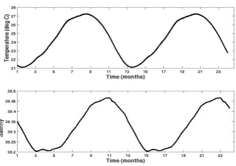
Figure 2. Time series of domain-averaged temperature (oC, top panel) and salinity
(bottom panel) for the last two years of the simulation.
Fig. 2. Time series of domain-averaged temperature (◦C, top panel) and salinity (bottom panel) for the last two years of the 20-year long simulation.
for variations of parameters (within reasonable range). An exception to this was the choice of the advection scheme for scalars (temperature and salinity). Highly diffusive advection schemes such as the upstream scheme produced an artificial, unwanted salinity trend in the Gulf of∼1 increase per year and were therefore discarded.
3 Results and discussion
3.1 Annual cycle of temperature und salinity
The predicted annual-mean surface-averaged evaporation rate is 1.8 m/yr, which is in agreement with previous esti-mates of Privett (1959), Hastenrath and Lamb (1979), Me-shal and Hassan (1986), and Ahmad and Sultan (1990). The annual-mean, surface-averaged heat flux is−4 W m−2, which agrees with the estimate of−7±4 W m−2by Johns et al. (2003). Gulf-averaged temperature and salinity attain a robust, steady seasonal cycle within 4–5 years of simulation time and onward (Fig. 2). Gulf-averaged temperature follows the seasonal cycle of incident solar radiation with a time lag of 1–2 months. Gulf-averaged salinity, on the other hand, attains minimum values during March-May each year. Ef-fects of precipitation and river run-off on salinity changes are negligible on a gulf-wide scale. Therefore, decreases in salinity can be fully attributed to inflow of IOSW that, in agreement with observational evidence, peaks in spring. Maximum salinities occur during October–December where the evaporative surface salinity flux dominates over injection of low-salinity water through the Strait of Hormuz.
3.2 Comparison with hydrographic field data
From the model results we have constructed temperature-salinity-season diagrams in different boxes along the Gulf for comparison with observational evidence (Alessi et al., 1999).
29
Figure 3. Locations of boxes used for detailed analysis of hydrographic properties.
Box 3
Box 7
Fig. 3. Locations of boxes used for detailed analysis of hydro-graphic properties.
This was done for all boxes defined by Alessi et al. (1999). To keep this paper short, we only discuss outcomes for the central Gulf region (Box 3) and for the Strait of Hormuz (Box 7). Figure 3 shows the location of these boxes. Note that in contrast to Alessi et al. (1999) our Box 3 includes shallow regions around Bahrain.
3.2.1 The Strait of Hormuz
The Strait of Hormuz region is exposed to inflow of IOSW and outflow of saline bottom water formed in different areas of the Persian Gulf that will be identified further below.
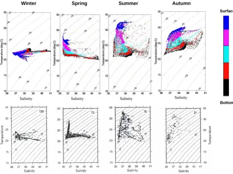
In winter, we encounter a situation of weak temperature contrasts in the Strait waters of <3◦C, but strong salin-ity differences of ∼4.5 (Fig. 4). Modified IOSW appears with a temperature of∼22◦C, a salinity of 36.5, and a den-sity of 1025.5 kg m−3. The dense outflow water attains a temperature of∼22.5◦C, a salinity of 41, and a density of 1028.5 kg m−3. Density in Strait waters ranges by 3 kg m−3. Note that temperature and salinity of the outflow are∼1◦C and∼0.5 too high as compared with field data (Johns et al., 2003).
30
Figure 4. Temperature-salinity-season diagram
s for the Strait of Hor
m
uz. (top) Model
predictions. Colours indicate sigm
a levels.
(bottom
) Field observations, taken from
Alessi
et al.
(1999).
Winter Spring Summer Autumn
Surface
Bottom
Salinity Salinity Salinity Salinity
Fig. 4. Temperature-salinity-season diagrams for the Strait of Hormuz. (top) Model predictions. Colours indicate sigma levels. (bottom) Field observations, taken from Alessi et al. (1999).
In summer, the salinity of the IOSW layer increases to 37– 38, while the surface temperature increases to>30◦C. The predicted salinity increase in surface water is associated with coverage of shallow regions off western Musandam Penin-sula (see Fig. 1) where evaporation forms water of slightly elevated salinities. Top-to-bottom temperature gradients ex-ceed 12◦C. We also find that intermediate water layers be-come saltier owing to diapycnal mixing. Interestingly, there is a warming of the most saline bottom waters by∼5◦C com-pared with the situation in spring. This warming is also seen in the field data (SB2003).
In autumn, the IOSW source water has become colder (see Table 3) and intense lateral and vertical mixing occurs in the Strait (and elsewhere in the Gulf). Lateral mixing is pro-vided by mesoscale eddies that start to form in this season (see below). Vertical mixing is associated with convective erosion of summer thermal stratification. As a result of this, the temperature of bottom water seen in the Strait increases to∼22◦C and the density of this water mass decreases to 1027.5 kg m−3. Density contrasts in the Strait decrease to 3.5 kg m−3. Owing to further cooling of the IOSW and
con-31
Figure 5. Seasonal variations of the density difference at both sides of the Strait of Hormuz at a depth level of ~70 m.
∆ρ
(kg m
-3)
Fig. 5. Seasonal variations of the difference in densities at both sides of the Strait of Hormuz at a depth level of∼70 m.
vective stirring, the seasonal cycle is completed to lead to winter conditions of relatively weak temperature contrasts, but haline stratification remains. Note the overall good agree-ment between field measureagree-ments and model predictions.
The baroclinic exchange circulation through the Strait of Hormuz is modified by the difference between the density of Gulf Bottom Water west of the Strait of Hormuz and that of water at comparable depths outside the Gulf. In our
34 J. K¨ampf and M. Sadrinasab: The circulation of the Persian Gulf
32
Figure 6. Sam
e as Fig. 4, but for central re
gions (Box 3) of the Persian Gulf.
Winter Spring Summer Autumn
Surface
Bottom
No data
Salinity Salinity Salinity Salinity
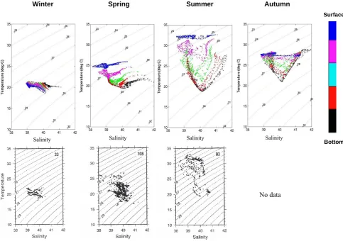
Fig. 6. Same as Fig. 5, but for central regions of the Persian Gulf.
simulation, this density difference peaks during February– May (Fig. 5). It has an average value of∼2.4 kg m−3 and varies by±40% over a year. In agreement with field obser-vations (SB2003), the density difference attains little vari-ations during February–May, whereas a significant change occurs from June to August associated with overall warm-ing of Gulf bottom water. Simulated volume transports of this outflow vary between∼0.17 Sv in spring and∼0.11 Sv in autumn, which is close to values reported by Johns et al. (2003). Obviously, density contrasts across the Strait modify the strength of the outflow, in consistency with hy-draulic theory (e.g. Pratt and Lundberg, 1991). Strengths of inflow and outflow are correlated to each other, so that the magnification of IOSW influx is driven by a stronger bottom outflow. This coupling can be explained by geostrophic ad-justment theory (see Appendix).
3.2.2 Central region of the Persian Gulf
In winter, waters of the central region of the Persian Gulf (Box 3) exhibit only little spatial variations in temperature of ∼1◦C (Fig. 6). Temperature is ∼20◦C, which is ∼2◦C
cooler compared with Strait water. There is a pronounced vertical salinity stratification with top-to-bottom salinity gra-dients of ∼1 and salinities span a range of 39–41, which includes lateral variations. Bottom water has a density of 1028.5–1029.5 kg m−3, which is slightly denser compared with bottom water found in the Strait (see Fig. 5).
In spring, local warming and import of warm (∼25◦C) modified IOSW leads to establishment of thermal stratifi-cation with top-to-bottom temperature differences of 6–7◦C. Surface water consists of modified IOSW that appears in this region with salinities in a range of 38–39, saline (values>40) waters forming in the shallow regions around Bahrain, and a water mass of salinities of 39–40 stemming from northwest-ern parts of the Gulf (see below). There is evidence of a water mass of temperatures of 19–20◦C, salinities of 40–41, and densities of 1028.8–1029 kg m−3, that SW2003 refer to as Gulf Deep Water. In agreement with SW2003, our simu-lation suggests that this water mass does only undergo slight variations in density over a year.
33
Figure 7. Lateral distributions of surface and bottom flow vectors (arrows, m s-1) over density (colours, sigma-t, kg m-3) averaged over summer months (June-August).
Surface
Bottom
33
Figure 7. Lateral distributions of surface and bottom flow vectors (arrows, m s-1) over
density (colours, sigma-t, kg m-3) averaged over summer months (June-August). Surface
Bottom
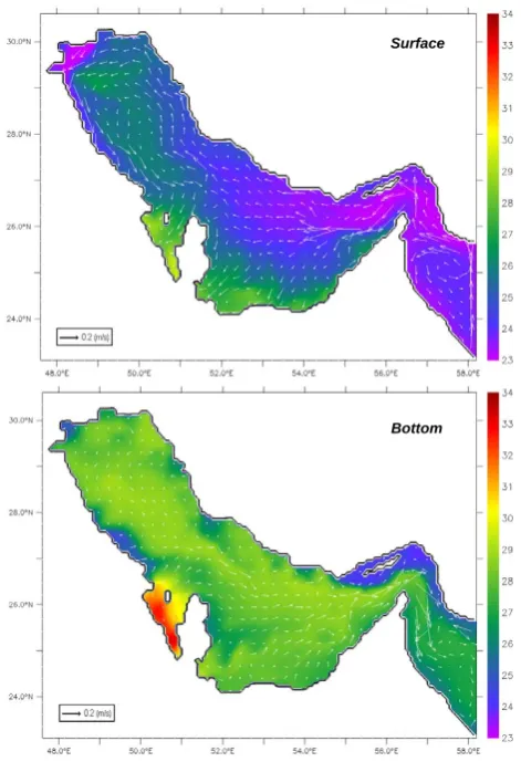
Fig. 7. Lateral distributions of surface and bottom flow vectors (ar-rows, m s−1)over density (colours, sigma-t units) averaged over summer months (June–August). Flow vectors are averaged over 5×5 grid cells for visualisation purposes.
waters from shallow regions around Bahrain, not captured by the field data, become warmer throughout the water column. In autumn, surface waters are cooled down to tempera-tures of∼27◦C, while the salinity range remains similar to that observed during summer. Mixing occurs between three water masses. These are 1) low-salinity modified IOSW, 2) high-salinity water formed around Bahrain, and 3) Gulf Deep Water. Owing to mixing the latter becomes slightly warmer by∼1◦C during autumn and its density increases slightly to 1028.4 kg m−3. River-derived surface water cannot be identi-fied in the temperature-salinity-season diagrams for the cen-tral region of the Gulf.
3.3 Seasonal variation of gulf-wide circulation
The circulation in the Persian Gulf displays an interesting seasonal behaviour. By summer, a cyclonic overturning cir-culation establishes along the full length of the gulf (Fig. 7). Under the influence of the Coriolis force, the surface inflow
34
Figure 8. Same as Fig. 7, but for autumn months (September-November).
Surface
Bottom
34
Figure 8. Same as Fig. 7, but for autumn months (September-November).
Surface
Bottom
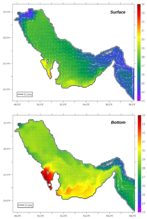
Fig. 8. Same as Fig. 7, but for autumn months (September– November).
through the Strait of Hormuz leans against the Iranian coast-line. This inflow (hereafter referred to as Iranian Coastal Jet or ICJ) has a pronounced bottom signature along the Iranian coast to a longitude of 55◦E, in agreement with longitudinal salinity transects presented by SB2003. To the west of this, the ICJ loses contact to the seafloor and turns into a buoy-ant surface flow. At the head of the Gulf, the ICJ joins the river plume fed by the Shatt-Al-Arab and flows back south-eastward along the coasts of Kuwait and Saudi Arabia. River discharge leads to formation of a classical river plume of a width of 30–40 km that, in summer, flows around Qatar and reaches western parts of the Southern Shallows. Tidal stir-ring dissolves the river plume with ambient water along the coast of Saudi Arabia. Local tidal mixing zones are also ev-ident along the Iranian coastline. Being surrounded by sur-face waters of lower salinity, a largely stagnant region estab-lishes in the centre of the northwestern part of the Gulf, in agreement with Reynolds (1993), that displays slightly ele-vated densities, stemming from eleele-vated salinities (see be-low). This region can be referred to as a salt plug (Wolanski,
36 J. K¨ampf and M. Sadrinasab: The circulation of the Persian Gulf
35
Figure 9. Same as Fig. 7, but for winter months (December-February)
Surface
Bottom
Fig. 9. Same as Fig. 7, but for winter months (December–February).
1986). Surface currents attain typical speeds of 10–20 cm/s. There are persistent south-westward surface currents in the southern regions of the Gulf away from Iran that turn into onshore (southward) flow in the Southern Shallows and near the shallows west of Qatar, in agreement with Hunter (1983). Summer densities in bottom layers are almost uniform, and dense bottom flow toward the Strait of Hormuz extends the entire length of the Gulf. The densest water is found in the shallows around Bahrain with values of>1033 kg m−3. This water becomes partially diluted with low-salinity water pro-vided by the river plume, but is seen to contribute to the dense bottom flow, in contrast to suggestions by SB2003. The bot-tom flow attains typical speeds of 5–10 cm/s, but magnifies to 20–30 cm/s past the Strait of Hormuz, in agreement with ADCP data (Johns and Olson, 1998; Johns et al., 2003). Bottom waters in the Southern Shallows do not display el-evated densities compared with ambient bottom waters and, therefore, do not significantly contribute to the driving of the dense bottom outflow in summer.
In autumn, where field data are lacking, the ICJ becomes dynamically unstable and forms meanders (Fig. 8). As a
36
Figure 10. Same as Fig. 7, but for spring months (March-May).
Surface
Bottom
36
Figure 10. Same as Fig. 7, but for spring months (March-May).
Surface
Bottom
Fig. 10. Same as Fig. 7, but for spring months (March–May).
result of this, the ICJ detaches from the Iranian Coast at a longitude of 51◦E. Autumn cooling produces relatively denser bottom water in the Southern Shallows which starts to contribute to driving of the dense bottom flow. The den-sity of this bottom water locally exceeds 1030 kg m−3 and mesoscale eddies form along a density front forming in the Southern Shallows along the 20-m depth contour. Dense wa-ter from the Southern Shallows becomes entrained into the dense bottom flow that still extends the full length of the Gulf.
37
Figure 11. Simulated surface salinities averaged over (top) summer months (June-August) and (bottom) winter months (December-February).
Summer surface salinity
Winter surface salinity
37
Figure 11. Simulated surface salinities averaged over (top) summer months (June-August) and (bottom) winter months (December-February).
Summer surface salinity
Winter surface salinity
Fig. 11. Simulated surface salinities averaged over (top) summer months (June–August) and (bottom) winter months (December– February).
spacing (∼20 km). Autumn and winter cooling has produced a very dense water mass in the Southern Shallows (density is>1032 kg m−3)that now, with some minor contribution of dense water formed around Bahrain, dominates the driv-ing of the dense bottom outflow toward the Strait of Hor-muz. Formation of this extremely dense water is associated with the existence of extensive shallow areas in the South-ern Shallows. Owing to advective delay, the result of this density increase is seen in the Strait of Hormuz in the pe-riod of January–May (see Fig. 4), so that there is a 3-month delay between the formation of anomalously dense water in the Southern Shallows and its appearance in the Strait. Note the injections of dense water from the Southern Shallows in form of narrow saline tongues inherent in mesoscale instabil-ities in the bottom layer. There is observational evidence of local lateral intrusion of saline, dense water stemming from the Southern Shallows (see Fig. 7a in SB2003). Deep flow in the north-western Gulf is largely absent in winter.
38
Figure 12. Close-up of lateral distributions of surface flow vectors (arrows, m s-1) over density (colours, sigma-t units) averaged over winter months (December-February). Spatial averaging has not been applied to flow vectors.
Fig. 12. Close-up of lateral distributions of surface flow vectors (ar-rows, m s−1)over density (colours, sigma-t units) averaged over winter months (December–February). Spatial averaging has not been applied to flow vectors.
In spring, when density differences across the Strait of Hormuz are at maximum, the ICJ starts to form and moves toward the head of the Gulf, but also intrudes the Southern Shallows (Fig. 10), in agreement with observational evidence (Reynolds, 1993; SB2003). Re-establishment of the river plume can be seen, and mesoscale baroclinic eddies have largely disappeared. Due to surface warming, the density excess of waters in the Southern Shallows gradually dimin-ishes, but still dominates the driving of the exchange circu-lation through the Strait. Bottom flows in the north-western Gulf are still negligibly weak.
The model simulations indicate that the winter/spring pe-riod is the pepe-riod in which the inflow of IOSW into the gulf starts to strengthen. During this time the front is spatially and temporally highly variable (see Figs. 9 and 10), and its location is not static. This makes it difficult to compare the climatologic mean location of the front, predicted by the model, with snapshot transects taken in February, as shown by Brewer and Dyrseen (1985) and Swift and Bowers (2003). Further field data are required to understand the complex na-ture of frontal development during this period for validation of our model prediction, which might have biases of timing of this inflow and of the strength of lateral mixing incurred by mesoscale frontal instabilities.
On the basis of axial density sections, SB2003 argue that the densest water of >1029.5 kg m−3 forms near the head of the Gulf and suggest that this density excess controls the density-driven circulation in the Persian Gulf. One major factor speaks against this hypothesis. North-south sections across the Gulf (Figs. 8a–b in SB2003) in winter show a sharp density increase toward the Southern Shallows where densities are>1030 kg m−3, exceeding values observed near the head. More importantly, the associated north-south
38 J. K¨ampf and M. Sadrinasab: The circulation of the Persian Gulf density gradients near the Southern Shallows establish over
a short distance of∼50 km and are thus 1 order of magni-tude stronger than those forming along the entire length of the Gulf (see Figs. 7a and 8b in SB2003). Thus, it is primar-ily this strong baroclinic north-south pressure gradient along the Southern Shallows that creates a swift geostrophic frontal flow and not that along the Gulf as previously suggested by SB2003.
Along the axes of the Gulf, our model findings for winter and spring show a slight density decrease in bottom water of ∼0.5 kg m−3 from the head to the centre and a density increase by∼1 kg m−3from the centre toward the Strait of Hormuz (see Figs. 9 and 10). In comparison with field data (see Fig. 7 of SB2003), the model appears to slightly over-estimate the density anomaly in the southern Gulf, which is associated with entrainment of hypersaline water from the Southern Shallows. This bias could be the result of too high evaporation rates in this area and/or too strong lateral turbu-lent mixing. Nevertheless, we deem this feature irrelevant because along-gulf pressure gradients are negligibly small compared with those establishing across the Gulf in vicin-ity of the Southern Shallows and therefore have only little effect on the dynamics.
3.4 Why the Persian Gulf is saltiest in winter
It has puzzled many generations of oceanographers that sur-face water of the Persian Gulf is, in general, saltier in winter than in summer, as also predicted with our model applica-tion (Fig. 11). Intensificaapplica-tion of the IOSW inflow in spring is a major reason why salinity in surface water along the Ira-nian coastline appears to be relatively low in summer. Es-tablishment of thermal stratification supports this process. In autumn and winter, together with a weakening of the IOSW inflow, the low-salinity surface signature partially disappears under the effects of lateral stirring of mesoscale eddies and convective deepening of the surface mixed layer. Previous suggestions for interannual salinity variations in surface wa-ter of the Persian Gulf include seasonal changes of 1) river discharge (Schott, 1908), 2) wind stress (Chao et al., 1992), 3) evaporation (Emery, 1956), and 4) evaporative lowering of sea surface height in the Gulf (SB2003). Findings of sensitiv-ity studies (not shown) indicate that neither of these factors have a significant impact on the seasonal cycle of circulation and water mass properties in the Persian Gulf. Instead of this, our simulations indicate that this seasonal cycle is asso-ciated with formation of dense bottom water in the Southern Shallows in autumn and winter (appearing in the Strait in late winter and spring) in conjunction with establishment of ther-mal stratification in spring. The formation of dense bottom water is due to surface cooling of extremely saline waters.
3.5 Circulation in the northern Gulf
During autumn and winter, our simulations indicate the es-tablishment of a persistent clockwise circulation pattern in the northern Gulf (Fig. 12) including a persistent south-eastward coastal jet along the Iranian coast with speeds of up to 10 cm/s. Existence of this coastal jet, forming dur-ing autumn (see Fig. 8), is in agreement with observational evidence (Reynolds 1993). During spring and summer this coastal jet is absent in the model simulation (see Figs. 7 and 10). Instead of this, the ICJ takes over to extend along the entire Iranian coastline. The summer circulation map, sug-gested by Reynolds (1993), could be biased by the occur-rence of a transient upwelling event during the time of the measurements, which is difficult to verify in the lack of suit-able meteorologic data. However, other evidences and, in particular, the effect on sediment transport (Uchupi et al., 1996) suggests that the formation of this coastal jet is, at least, recurrent. It should be kept in mind that our model is driven by monthly mean atmospheric forcing, which ex-cludes the description of synoptic-scale upwelling events and effects caused by strong diurnal winds associated with sea breezes over the Gulf. These features might lead to estab-lishment of a quasi-permanent coastal jet in summer, absent in our simulations.
4 Conclusions
Findings presented in this paper and summarised in the fol-lowing provide new insight into seasonal variations of the cir-culation and water mass properties in the Persian Gulf. Our results, which are in good agreement with previous hydro-graphical data, suggest the following.
J. K¨ampf and M. Sadrinasab: The circulation of the Persian Gulf 39 autumn and winter and breaks up into mesoscale eddies, so
that the ICJ disappears. Lateral mixing by eddies and ver-tical mixing due to convective removal of the summer ther-mal stratification contributes to the fact that surface Gulf wa-ters appear more saline in autumn and winter compared with spring and summer. Dense water formed around Bahrain only marginally contributes to the driving of the deep flow owing to dilution with river-derived low-salinity water and small volume compared to the Southern Shallows.
To further improve understanding of the circulation in-cluding seasonal variations in the Persian Gulf, more field observations are required to close data gaps that exist for autumn months for the entire Gulf and year-round for the Southern Shallows. Also required is a better knowledge of current river discharge rates of the Shatt-al-Arab.
Future theoretical studies should investigate effects of both varied river discharge and synoptic-scale wind and heat-flux forcing on the circulation in the Persian Gulf. The focus hereby should be placed into investigation of 1) heat fluxes and dense water formation in the Southern Shallows and 2) atmospheric conditions that promote formation of a coastal jet along the Iranian coast in the northern Gulf, not ade-quately described in our model simulations, and how this in-teracts with the gulf-wide circulation.
Appendix A
Simple dynamical model of frontal flow through a strait
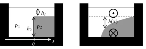
Simple geostrophic adjustment theory for a two-layer frontal flow is considered to explain the coupling between magni-tudes of inflow and outflow through the Strait of Hormuz. To this end, we consider the initial configuration of a wall of dense water of heighth0 with a density anomaly of1ρ leaning against the right-hand bank of a Strait of depth H
(Fig. A1).
The steady-state dynamical equations suitable to tackle this problem are the geostrophic equations and conserva-tion of potential vorticity (see Cushman-Roisin, 1994). The geostrophic relations (see Fig. A1) are given by:
f v1=g ∂η
∂x , (A1)
f v2= ρ1 ρ2
g∂η ∂x −g
0∂h
∂x ≈g ∂η ∂x −g
0∂h
∂x, (A2)
where indices 1 and 2 refer to the upper and lower layer, respectively, η is the resultant sea surface elevation, and
g0=(ρ2−ρ1)/ρ2g is reduced gravity. Note that the Boussi-nesq approximation (ρ2/ρ1≈1) is used in Eq. (A2). Conser-vation of potential vorticity requires
f+∂v1/∂x h1+h
= f
h1 ⇒∂v1
∂x =
f h1
h , (A3)
39
Simple geostrophic adjustment theory for a two-layer frontal flow is considered to explain the coupling between magnitudes of inflow and outflow through the Strait of Hormuz. To this end, we consider the initial configuration of a wall of dense water of height ho with a density anomaly of ∆ρ leaning against the right-hand bank of a Strait
of depth H (Figure A1).
Figure A1: Schematic of geostrophic adjustment of a two-layer density front in a Strait. a) Initial configuration. b) Baroclinic frontal flow and return flow in the upper ocean.
The steady-state dynamical equations suitable to tackle this problem are the geostrophic equations and conservation of potential vorticity (see Cushman-Roisin 1994). The geostrophic relations (see Fig. A1) are given by:
x g fv ∂ ∂ = η
1 , (A1)
x h g x g x h g x g fv ∂ ∂ − ∂ ∂ ≈ ∂ ∂ − ∂ ∂ = ' ' 2 1 2 η η ρ
ρ , (A2)
where indices 1 and 2 refer to the upper and lower layer, respectively, η is the
resultant sea surface elevation, and g’=(ρ2-ρ1)/ρ2 g is reduced gravity. Note that the
Boussinesq approximation (ρ2/ρ1 ≈ 1) is used in (A2). Conservation of potential
vorticity requires ρ2 h2 h(x) x ρ1 h1 0
Fig. A1. Schematic of geostrophic adjustment of a two-layer den-sity front in a Strait. (a) Initial configuration. (b) Baroclinic frontal flow and return flow in the upper ocean.
f +∂v2/∂x h2−h
= f
h2 ⇒ ∂v2
∂x = −
f h2
h , (A4)
where small changes in total water depth owing to sea level variations have been ignored; that is, the rigid-lid approx-imation has been employed. A combination of the latter Eqs. (A1–A4) gives:
∂2h ∂x2 =
f2
g0Hh (A5)
with the equivalent depth being defined as
H=h1h2/(h1+h2). The solution of Eq. (A5) is: h(x)=
h2exp[−(x+R)/R] ; x ≥ −R
h2 ; x <−R
(A6) where the internal deformation radius is given by
R=√[(g0H )]/f. From Eqs. (A3) and (A4), we yield:
v2(x)=
p
g0Hexp[−(x+R)/R] ; x≥ −R
0 ; x <−R (A7)
v1(x)= − h2 h1
v2. (A8)
Furthermore, inserting Eq. (A8) in (A1) gives the resultant sea level elevation:
η(x)=
−η0{1−exp[−(x+R)/R]} ; x ≥ −R
0 ; x <−R ; (A9)
whereη0=(ρ2−ρ1)/ρ2h22/(h1+h2). According to the above solutions, volume transports in the upper and lower layer can be calculated as:
Q2= ∞
Z
−R
v2(h2−h)dx=0.5
p g0H h
2R , (A10)
Q1= ∞
Z
−R
v1(h1+h)dx
= −pg0H h
2R(1+0.5h2/ h1)
= −2Q2(1+0.5h2/ h1) . (A11)
40 J. K¨ampf and M. Sadrinasab: The circulation of the Persian Gulf The two latter equations suggest that, in the absence of other
processes, the magnitude of the inflow would always exceed that in the lower layer by a factor >2. This implies that in a semi-enclosed estuary, such as the Persian Gulf, and for comparatively small evaporative losses, the sea level in the estuary would increase over time creating a barotropic pressure gradient along the Strait. This pressure gradient, in turn, would create an additional barotropic flow compo-nent through the Strait such that inflow and outflow attain volume transports of the same order of magnitude. The re-sultant steady-state volume transports can be derived as the average of magnitudes of Eqs. (A10) and (A11), yielding:
Q2≈0.5
p g0H h
2R(1.5+0.5h2/ h1) , (A12)
Q1= −Q2. (A13)
For parameters characterizing the
ex-change flow through the Strait of Hormuz
(p(g0H )≈0.5 m/s, h
2≈40 m, R≈7.7 km, h2/ h1≈1), Eq. (A12) yields an estimate of the volume transport of the outflow of Q2≈0.15 Sv, with the inflow carrying approxi-mately the same amount of water, which is of the order of magnitude as estimated by Johns et al. (2003). The overall essence of this consideration is that geostrophic adjustment of a density front in a Strait triggers a return flow in upper layers of the water column of a magnitude being correlated with that of the frontal outflow current.
Acknowledgements. This work was supported by an international postgraduate scholarship awarded by Khorramshahr University of Marine Sciences & Technology, Iran, and a grant from Flinders University, South Australia. We thank SAPAC (South Australian Partnership of Advanced Computing) for provision of their facili-ties and for technical support. We are grateful to M. Tomczak and the referees for helpful suggestions that improved this paper.
Edited by: E. J. M. Delhez
References
Ahmad, F. and Sultan, S. A. R.: Annual mean surface heat fluxes in the Arabian Gulf and the net heat transport through the Strait of Hormuz, Atmos. Ocean., 29, 54–61, 1991.
Alessi, C. A., Hunt, H. D., and Bower, A. S.: Hydrographic data from the U.S. Naval Oceanographic Office: Persian Gulf, South-ern Red Sea, and Arabian Sea 1923–1996, Woods Hole Oceanog. Inst. Tech. Rep., WHOI-99-02, 1999.
Arakawa, A. and Suarez, M. J.: Vertical differencing of the primi-tive equations in sigma coordinates, Mon. Wea. Rev., 111, 34–45, 1983.
Bashir, M., Khaliq, A. Q. M., and Al-Hawaj, A. Y.: An explicit finite difference, model for tidal flows in the Arabian Gulf, in: Computational techniques and applications: CTAC-89, edited by: Hogarth, W. L. and Noye, B. J., Griffith University, Bris-bane, Queensland, Australia, Hemisphere Publishing Corp., New York, 295–302, 1989.
Blumberg, A. F. and Mellor, G. L.: A description of a three-dimensional coastal ocean circulation model, in: Three-dimensional Coastal Ocean Models, edited by: Heaps, N. S., Coastal and Estuarine Sciences, vol. 4, American Geophysical Union, Washington D.C., 1–16, 1987.
Brewer, P. G. and Dyrssen, D.: Chemical Oceanography of the Per-sian Gulf, Prog. Oceanog., 14, 41–55, 1985.
Chao, S.-Y., Kao, T. W., and Al-Hajri, K. R.: A numerical investi-gation of circulation in the Arabian Gulf, J. Geophys. Res., 97, 11 219–11 236, 1992.
Cushman-Roisin, B.: Introduction to Geophysical Fluid Dynamics, Prentice-Hall, Englewood Cliffs, N. J., 1994.
El-Shabh, M. I. and Murty, T. S.: Simulation of the movement and dispersion of oil slicks in the Arabian Gulf, Nat. Hazards, 1, 197– 219, 1988.
Emery, K. O.: Sediments and water of the Persian Gulf, AAPG Bull., 40, 2354–2383, 1956.
Galperin, B., Kantha, L. H., Hassid, S., and Rosati, A.: A quasi-equilibrium turbulent energy model for geophysical flows, J. At-mos. Sci., 45, 55–62, 1988.
Geernaert, G. L., Katsaros, K. B., and Richter, K.: Variation of the drag coefficient and its dependence on sea state, J. Geophys. Res., 91, 7667–7679, 1986.
Hastenrath, S. and Lamb, P. J.: Climatic atlas of the Indian Ocean, Part 2, The ocean heat budget, Univ. of Wisc. Press, Madison, Wisconsin, 1979.
Hunter, J. R.: The physical oceanography of the Arabian Gulfs: a review and theoretical interpretation of previous observations, Marine Environment and Pollution, Proceedings of the First Ara-bian Gulf Conference on Environment and Pollution, Kuwait, 7– 9 February 1982, 1–23. 1982.
Hunter, J. R.: Aspects of the dynamics of the residual circulation of the Arabian Gulf, in: Coastal oceanography, edited by: Gade, H. G., Edwards, A., and Svendsen, H., Plenum Press, 31–42, 1983. Johns, W. E. and Olson, D. B.: Observations of seasonal exchange
through the Strait of Hormuz, Oceanography, 11, 58, 1998. Johns, W. E., Yao, F., Olson, D. B., Josey, S. A., Grist, J.
P., and Smeed, D. A.: Observations of seasonal exchange through the Straits of Hormuz and the inferred freshwater bud-gets of the Persian Gulf, J. Geophys. Res., 108(C12), 3391, doi:10.1029/2003JC001881, 2003.
Landner, R. W., Belen, M. S., and Cekirge, H. M.: Finite differ-ence model for tidal flows in the Arabian Gulf, Computers and Mathematics with Applications, 8(6), 425–444, 1982.
Le-Provost, C.: Models for tides in the KAP region, in: Oceano-graphic modelling of the Kuwait Action Plan (KAP) region, edited by: El-Sabh, M. I., UNESCO Rep. in Marine Science, 28, 37–45, 1984.
Luyten, P. J., Jones, J. E., Proctor, R., Tabor, A., Tett, P., and Wild-Allen, K.: COHERENS – A coupled hydrodynamical-ecological model for regional and shelf seas: user documentation, MUMM Rep., Management Unit of the Mathematical Models of the North Sea, 1999.
Mellor, G. L. and Yamada, T.: Development of a turbulence clo-sure model for geophysical fluid problems, Rev. Geophys. Space Phys., 20, 851–875, 1982.
Mesinger, F. and Janji, Z. I.: Problems and numerical methods of the incorporation of mountains in atmospheric models, Lectures in Applied Mathematics, 22, 81–121, 1985.
Najafi, H. S.: Modelling tides in the Persian Gulf using dynamic nesting, PhD thesis, University of Adelaide, Adelaide, South Australia, 1997.
Oey, L.-Y. and Chen, P.: A model simulation of circulation in the Northeast Atlantic shelves and seas, J. Geophys. Res., 97, 20 087–20 115, 1992.
Perrone, T. J.: Winter shamal in the Persian Gulf, Tech. Rep., Naval Environ. Predict. Res. Facil., Monterey, Calif., 79–06, 1979. Pratt, L. J. and Lundberg, P. A.: Hydraulics of rotating strait and sill
flows, Annual Review of Fluid Mechanics, 23, 81–106, 1991. Privett, D. W.: Monthly charts of evaporation from the North Indian
Ocean, including the Red Sea and the Persian Gulf, Quart. J. Roy. Meteorol. Soc., 85, 424–428, 1959.
Proctor, R., Eliott, A., and Flather, R. A.: Modelling tides and sur-face drift in the Arabian Gulf-Application to the Gulf oil spill, Cont. Shelf Res., 14, 531–545, 1994.
Reynolds, R. M.: Physical oceanography of the Gulf, Strait of Hor-muz, and the Gulf of Oman – Results from the Mt Mitchell ex-pedition, Mar. Pollution Bull., 27, 35–59, 1993.
Saad, M. A. H.: Seasonal variations of some physiochemical con-dition of Shatt-al-Arab estuary, Iraq, Estuarine Coastal Mar. Sci., 6, 503–513, 1978.
Sadrinasab, M. and K¨ampf, J.: Three-dimensional flushing times in the Persian Gulf, Geophys. Res. Letters, 31, L24301, doi:10.1029/2004GL020425, 2004.
Schott, G.: Oceanographie and Klimatologie des Persischen Golfes und des Golfes von Oman, Ann. Hydrogr. Mar. Meteorol., 46, 1–46, 1918.
Seibold, E. and Ulrich, J.: Zur Bodengestalt des nordwestlichen Golfs von Oman. “Meteor” Forsch. Ergebnisses, Reihe C, 3, 1– 14, 1970.
Sielecki, A.: An energy-conserving finite difference scheme for the storm surge equations, Mon. Wea. Rev., 96, 150–156, 1968. Smagorinsky, J.: General circulation experiments with the primitive
equations. The basic experiment, Mon. Wea. Rev., 91, 99–165, 1963.
Sugden, W.: The hydrology of the Persian Gulf and its significance in respect to evaporite deposition, Amer. J. Sci., 261, 741–755, 1963.
Swift, S. A. and Bower, A. S.: Formation and circulation of dense water in the Persian/Arabian Gulf, J. Geophys. Res., 108(C1), 3004, doi:10.1029/2002JC001360, 2003.
UNESCO: Tenth report of the joint panel on oceanographic tables and standards, UNESCO Tech. Pap. in Marine Sci., No. 36, UN-ESCO, Paris, 1981.
Uchupi, E., Swift, S. A., and Ross, D. A.: Gas venting and late quaternary sedimentation in the Persian (Arabian) Gulf. Marine Geology, 129, 237–269, 1996.
Wolanski, E.: An evaporation-driven salinity maximum zone in Australian tropical estuaries, Estuarine, Coastal and Shelf Sci-ence, 22, 415–424, 1986.
Wright, J. L.: A hydrographic and acoustic survey of the Persian Gulf, MSc Thesis, Nav. Postgrad. Sch., Monterey, Calif., 1974.