Upper ocean response to the passage of two sequential typhoons

www.ocean-sci.net/10/559/2014/ doi:10.5194/os-10-559-2014

© Author(s) 2014. CC Attribution 3.0 License.

Upper ocean response to the passage of two sequential typhoons

D. B. Baranowski1, P. J. Flatau2, S. Chen3, and P. G. Black4

1_{Institute of Geophysics, Faculty of Physics, University of Warsaw, Warsaw, Poland}

2_{Scripps Institution of Oceanography, University of California San Diego, San Diego, CA, USA} 3_{Naval Research Laboratory, Monterey, CA, USA}

4_{Science Applications International Corporation, Monterey, CA, USA}

Correspondence to: D. B. Baranowski ([email protected])

Received: 8 October 2013 – Published in Ocean Sci. Discuss.: 2 December 2013 Revised: 21 March 2014 – Accepted: 28 April 2014 – Published: 30 June 2014

Abstract. The atmospheric wind stress forcing and the oceanic response are examined for the period between 15 September 2008 and 6 October 2008, during which two typhoons – Hagupit and Jangmi – passed through the same region of the western Pacific at Saffir–Simpson intensity categories one and three, respectively. A three-dimensional oceanic mixed layer model is compared against the remote sensing observations as well as high-repetition Argo float data. Numerical model simulations suggested that magni-tude of the cooling caused by the second typhoon, Jangmi, would have been significantly larger if the ocean had not al-ready been influenced by the first typhoon, Hagupit. It is es-timated that the temperature anomaly behind Jangmi would have been about 0.4◦C larger in both cold wake and left side of the track. The numerical simulations suggest that the magnitude and position of Jangmi’s cold wake depends on the precursor state of the ocean as well as lag between ty-phoons. Based on sensitivity experiments we show that tem-perature anomaly difference between “single typhoon” and “two typhoons” as well as magnitude of the cooling strongly depends on the distance between them. The amount of ki-netic energy and coupling with inertial oscillations are im-portant factors for determining magnitude of the tempera-ture anomaly behind moving typhoons. This paper indicates that studies of ocean–atmosphere tropical cyclone interaction will benefit from denser, high-repetition Argo float measure-ments.

1 Introduction

In recent years understanding the predictability of tropical cyclone formation, intensification, and structure change has been a subject of intense interest. On the experimental front, THe Observing system Research and Predictability EXperi-ment (THORPEX) has concentrated on improving the skill of 1–14-day forecasts of high-impact weather. Throughout the THORPEX program, several regional campaigns have been undertaken to address these events. One such multi-national program was conducted during August–September 2008 over the western North Pacific (WPAC) as the summer com-ponent of THORPEX Pacific Asian Regional Campaign in collaboration with the Office of Naval Research (ONR)-sponsored Tropical Cyclone Structure 2008 experiment, re-ferred to as TPARC/TCS08. The focus of TPARC/TCS08 has been on various aspects of typhoon activity, including forma-tion, intensificaforma-tion, structure change, moforma-tion, and extratrop-ical transition (Elsberry and Harr, 2008). Another recent joint program – The Impacts of Typhoons on the Ocean in the Pa-cific and Tropical Cyclone Structure 2010 (ITOP/TCS10) – took place during September–October 2010 also in WPAC (D’Asaro et al., 2011). It too was a multi-national field cam-paign that aimed to study the ocean response to typhoons in the western Pacific Ocean with scientific objectives related to the formation and dissipation of typhoon cold wakes, the magnitude of air–sea fluxes for winds greater than 30 m s−1_, the influence of ocean eddies on typhoons, the surface wave field under typhoons, and typhoon genesis in relation to envi-ronmental factors. These projects built upon the earlier air– sea interaction observations obtained in the Atlantic during the Coupled Boundary Layer Air-Sea Transfer (CBLAST) experiment conducted in the western Atlantic (Black et al., 2007).

boundary layer (Wu et al., 2007; Cione and Uhlhorn, 2003; Ramage, 1974) and the biology and chemistry of the upper ocean (Babin et al., 2004; Lin et al., 2003). The wake de-velopment itself depends on complex non-linear atmospheric forcing related to the tropical cyclone size, strength and tran-sitional speed as well as background ocean conditions like the upper ocean stratification and depth of the thermocline (Price et al., 1994; Hong et al., 2007; Schade and Emanuel, 1999). Based on observations, data analysis (Uhlhorn and Shay, 2011), and modeling (Uhlhorn and Shay, 2013), it has been shown that preexisting upper ocean kinetic energy structure plays also an important role in the ocean response to the tropical cyclone forcing.

Even though some progress towards understanding the oceanic response to cyclone passage has been recently doc-umented, direct measurements of the oceanic state for such events are limited (D’Asaro et al., 2007, 2011; Mrvaljevic et al., 2013). As the tropical cyclone development and intensi-fication is sensitive to the sea surface temperature (SST) (Wu et al., 2007; Emanuel et al., 2004), it follows that cold wakes would likely affect the development and intensification of subsequent tropical cyclones that happen to follow a simi-lar track to their predecessor within a short period of time. Interactions and interlinks between two tropical cyclones oc-curring in vicinity of each other have been recognized as an important forecasting issue (Brand, 1971; Falkovich et al., 1995), but more detailed studies have become available only in recent years (Wada and Usui, 2007). These studies indi-cate that upper ocean thermal and energy structure disturbed by the preceding cyclone might influence the evolution of the following cyclone. Therefore, the proper assessment of the upper ocean heat content, which represents upper ocean thermal structure, is important for tropical cyclone forecast-ing systems, includforecast-ing forecasts of initiation, evolution, tra-jectory and foremost intensification. The interaction of two cyclones closely related in time and space thus provides a natural laboratory for studying ocean response and cold wake persistence.

To our knowledge, the question of how the cold wake of the trailing typhoon might change as a result of the dis-turbed oceanic state generated by its predecessor has not been previously addressed. Such an interaction might be im-portant for proper assessment and forecast of ocean stratifi-cation, SST and evolution of atmospheric convection. In this

of two consecutive typhoons.

We begin with climatology of the region in Sect. 2 in an effort to define the basic state of the ocean that existed prior to the passage of the typhoon couplet of interest in this study. This is followed by description of the Argo data as well as the ocean model and wind fields used to conduct numerical simulations of the cold wake dynamics. The in situ obser-vations of mixed layer (ML) evolution as obtained by the daily JAMSTEC Argo float are presented in Sect. 3, while Sect. 4 presents modeling results, which include the compar-ison model runs and numerical experiments. A summary of the primary results and discussion can be found in Sect. 5.

2 Oceanic state and description of methods 2.1 Basic oceanic state

WPAC has the largest number and frequency of tropical cyclones (TCs) of all the ocean basins (Frank and Young, 2007). During the typhoon season in this basin, which usu-ally lasts from mid-July until mid-November, there are typ-ically around 30 tropical cyclones (TCs), half of which achieve typhoon strength (Lander, 1994). Our analysis of the typhoon tracks in WPAC during 2000 to 2010 shows there were a total of 288 TCs, of which 33 % had recurring tracks (defined as those TCs that are separated temporally by no more than a 2-week period and exhibit storms tracks that lie no more than 100 km apart (Fig. 1)). Of the TCs reaching the typhoon stage, 17 % (or 32 typhoons) were found to have recurring tracks. While the use of more stringent search crite-ria of 50 km reduces the number of repeating storms to about 10 % (28 typhoons), it is clear that, on average, there was more than one pair of typhoons exhibiting repeating tracks for this basin in each season examined.

For the recurring typhoons there is generally only a short period of time for the ocean to fully recover to the ini-tial undisturbed state prior to the passage of the subsequent storm. One thus expects in such cases that the oceanic mixed layer (ML) encountered by the trailing storm is perturbed and may have an impact on the subsequent typhoon devel-opment. In a effort to establish the undisturbed conditions for our subsequent analyses, the mean temperature, salin-ity and denssalin-ity profiles from the Argo-based climatology

19 1

2

Fig.1. Climatology of 288 Western Pacific typhoon tracks during year 2000 to 2010 and SST 3

climatology for September (top panel) and the number of recurring tracks for each year 4

(bottom panel). Two criteria of track radius, 50 and 100 km, were used to compute the 5

statistics. On the top panel tracks of typhoons Hagupit and Jangmi are black solid lines. 6

Figure 1. Climatology of 288 western Pacific typhoon tracks during

year 2000 to 2010 and SST climatology for September (top panel) and the number of recurring tracks for each year (bottom panel). Two criteria of track radius, 50 and 100 km, were used to com-pute the statistics. On the top panel tracks of typhoons Hagupit and Jangmi are black solid lines.

(Roemmich and Gilson, 2009) were computed for the 1 de-gree×1 degree box region centered at 17.5◦N, 126.5◦E that corresponds to the mean location for our area of interest (Fig. 2). This data set is based on Argo profiles for years 2004–2012 and shows the overall time-mean profiles along with their standard deviation for the month of September (given by the grey curves in the plot). When these longer term climatological profiles are compared with the condi-tions during September 2008 associated with the develop-ment of Hagupit and Jangmi, we find that the ocean state ac-companying these storms was warmer and less salty by ap-proximately one and two standard deviations, respectively. Climatological SST for September based on the same data set is shown in Fig. 1; SST in the area of interest is hori-zontally uniform. Typhoon Hagupit passed through the anal-ysis region on 21 September as a Saffir–Simpson category (CAT) 1 typhoon followed by the CAT 3 typhoon Jangmi on

20 1

2

Fig.2. Monthly Climatology of temperature, salinity and density from Argo based climatology 3

(Roemmich and Gilson 2009) for the 1×1 degree grid centered at 17.5N, 126.5E. Solid grey 4

line represents the mean value and dashed grey lines represent deviation from the mean 5

(standard deviation). Solid black line shows the September 2008 value. 6

7

Figure 2. Monthly climatology of temperature, salinity and density

from Argo-based climatology (Roemmich and Gilson, 2009) for the 1 degree×1 degree grid centered at 17.5◦N, 126.5◦E. Solid grey line represents the mean value, and dashed grey lines represent de-viation from the mean (standard dede-viation). Solid black line shows the September 2008 value.

26 September (see Figs. 3 and 4, respectively). The passage of the Hagupit–Jangmi typhoon pair was itself preceded in this area by developing typhoon Sinlaku in early September and typhoon Nuri in mid-August. While precipitation from the Hagupit–Jangmi typhoon pair may have itself contributed to a fresher than usual ML, we suspect that September 2008 was less salty than normal due to the passage through the same area by these two previous typhoons. Sinlaku devel-oped into a tropical storm on 8–9 September passing through the middle of the region only 12 days prior to Hagupit. Ty-phoon Nuri, meanwhile, passed through the northern portion of the region as a CAT 1 intensity storm on 19 August. The Naval Research Laboratory (NRL) microwave satellite im-agery (http://www.nrlmry.navy.mil/tc-bin/tc_home2.cgi) for Sinlaku showed that the eye of this storm was just develop-ing and was associated with weaker rainbands that passed through the analysis area. The Nuri imagery indicated that the heaviest precipitation region associated with this typhoon was centered over the southern portion of our area of inter-est. Therefore, the winds over this region would have been light during both of these events, but the rainfall would likely have been extensive and heavy, probably resulting in the less saline conditions for September 2008 but with very little ML modification due to wind forcing.

2.2 Argo data

Of the large number of Argo floats present in the western Pacific region in September 2008, only one happened to be fortuitously located right between the two sequentially oc-curring typhoons Hagupit and Jangmi. This instrument, float ID 5901579, was deployed by JAMSTEC as part of the PALAU2008 field program and was set to conduct a verti-cal profile of the ocean from a depth of 500 m to the sur-face everyday. This float was initially released from R/V

Mi-rai and was intended to measure air–sea interactions with

21

1

2

Fig. 3. The wind speed [m/s] and wind direction (blue arrows) at 06Z on September 21, 2008.

3

The best track of typhoon Hagupit is plotted as the magenta line with the diamonds denoting

4

the 12 hour storm position. The white circles indicate the daily Argo float locations between

5

September 18 and September 29, 2008.

6

7

Figure 3. The wind speed [m s−1] and wind direction (blue arrows) at 06Z on 21 September 2008. The best track of typhoon Hagupit is plotted as the magenta line with the diamonds denoting the 12 h storm position. The white circles indicate the daily Argo float loca-tions between 18 September and 29 September 2008.

22

1

2

Fig. 4. The wind speed [m/s] and wind direction (blue arrows) on September 26, 2008. The

3

best track position of typhoon Jangmi is plotted as the magenta line with diamonds denoting

4

the 12 position of the storm center. The white circles indicate the daily Argo float locations

5

between September 18 and September 29, 2008.

6

7

Figure 4. The wind speed [m s−1] and wind direction (blue arrows) on 26 September 2008. The best track position of typhoon Jangmi is plotted as the magenta line with diamonds denoting the 12 position of the storm center. The white circles indicate the daily Argo float locations between 18 September and 29 September 2008.

the particular objective of improving understanding of intra-seasonal variations in the western Pacific. For that reason it was set up to take one profile everyday with the vertical res-olution of about 5 m from the ocean surface down to 200 m; below 200 m the float’s resolution is about 10 m. The data

23

1

2

Fig. 5. Position of the Argo Float ID 5901579 between September 1 and October

10 with

3

respect to the typhoon Hagupit (diamonds) and Jangmi (circles) best tracks. The various

4

symbols represent different group time periods as denoted on the plot.

5

6

Figure 5. Position of the Argo float ID 5901579 between 1

Septem-ber and 10 OctoSeptem-ber with respect to the typhoon Hagupit (diamonds) and Jangmi (circles) best tracks. The various symbols represent dif-ferent group time periods as denoted on the plot.

obtained thus provide a unique opportunity to study daily changes in the upper ocean during the sequential passage of these two active typhoons. Only data flagged “good” are used; therefore some data points are skipped. Presence of this particular instrument at that time and location was highly for-tunate. Both typhoons Hagupit and Jangmi were intensively studied as part of TPARC/TCS08 field campaign, but none of the instruments deployed as part of targeted measurements were in the position to measure response to repeated typhoon passages.

Figure 5 shows that the float was located near 17.5◦N, 126.5◦E during the month of September 2008 and exhib-ited overall displacements less than 100 km during the 20-day period during which Hagupit and Jangmi passed through the area. From Figs. 3 and 4 we see that this float was po-sitioned about 40 km to the right of the track of typhoon Hagupit and approximately 100 km to the left of the track of typhoon Jangmi. It was thus ideally situated for use in sub-sequent analyses of the cold wake as well as input for use in the idealized model studies that we describe next.

2.3 The three-dimensional Price–Weller–Pinkel (3DPWP) ocean model

A three-dimensional, primitive-equation, hydrostatic numer-ical ocean model (3DPWP) (Price et al., 1994, 1986) is used for numerical simulations of the cold wakes examined in this study. The model runs were performed with a 5 km horizontal resolution and a variable vertical grid resolution that was set

Table 1. Description of the numerical experiments.

Experiment Initial ocean Number of Number of name condition typhoons model simulations

HH Hagupit 1 1

JJ Jangmi 1 1

HJ Hagupit 1 1

HHJ Hagupit 2 5

HHH Hagupit 2 10

to 5 m between the surface and 100 m, and a constant 10 m resolution below a depth of 100 m. The total domain depth was set to 2000 m. The model was initialized with the wind field obtained from Cooperative Institute for Research in At-mosphere (CIRA) as the surface forcing (Figs. 3 and 4) and employed the drag coefficient defined by Powell et al. (2003). The model initial ocean conditions were assumed to be horizontally homogenous and correspond to the undisturbed Argo profile shown in Fig. 6. Five model experiments were performed – two control simulations and three sensitivity ex-periments (Table 1). For the “control” simulation, typhoon Hagupit (hereafter referred to as HH) was initialized based on the pre-Hagupit ocean conditions. The typhoon Jangmi control case (hereafter referred to as JJ) was initialized from the pre-Jangmi oceanic conditions. These simulations were performed to establish the model’s three-dimensional ocean response from these two TC forcings. They are compared with in situ observations from Argo float and the sensitiv-ity experiments. The sensitivsensitiv-ity “experiment 1” (HJ) is the same as the Jangmi control except the initial ocean is from the pre-Hagupit conditions. Sensitivity “experiment 2” sim-ulates two sequential typhoons, and it was initialized with the pre-Hagupit conditions (HHJ). The two model typhoon trajectories are separated by 140 km, which corresponds to the observed track distance between these two typhoons (see Fig. 5). In the final set of experiments, we investigate the ocean’s response to two identical Hagupit-like forcings fol-lowing the same track but separated by 55–195 h in time. Pre-Hagupit conditions are used as initial conditions in this experiment (HHH).

For the “pre-Hagupit” conditions, the Argo profile for 19 September is used, and for the “pre-Jangmi” conditions the profile from 25 September is used (Fig. 6). The transla-tional velocity of the typhoon is set to 6 m s−1_{in all} numeri-cal experiments based on the best tracks data from Japan Me-teorological Agency (JMA) and Joint Typhoon Warning Cen-ter (JTWC). These assumptions reproduced a good agree-ment between the model and 6 hourly CIRA wind speeds at the Argo float location (Fig. 7).

For the control simulations HH and JJ, we compare the mixed layer temperature (MLT), temperature tendencies, mixed layer depth (MLD), and stratification in the thermo-cline. We exercised some care when doing such direct model

24 1

2

Fig. 6. The initial temperature [C], salinity [psu], and density [kg/m3_{] profiles used in the} 3

3DPWP simulations HH and HJ (circles) and JJ (squares) described in the text. The dashed 4

black lines show the mean climatology profiles with added and subtracted standard deviations 5

for September, 2008. 6

7

Figure 6. The initial temperature [◦C], salinity [psu], and density [kg m−3] profiles used in the 3DPWP simulations HH and HJ (cir-cles) and JJ (squares) described in the text. The dashed black lines show the mean climatology profiles with added and subtracted stan-dard deviations for September 2008.

25 1

2

Fig. 7. Wind speed as a function of time at the Argo float location (17.5°N, 126.5°E) based on 3

observations and model results. The dots and diamonds represent CIRA data for typhoons 4

Hagupit and Jangmi every 6h. The dashed and dotted lines are wind speeds used in the model 5

forcing (based on only one initial velocity field, but advected with the center of TC 6

movement) for typhoons Hagupit and Jangmi respectively. 7

8

Figure 7. Wind speed as a function of time at the Argo float location

(17.5◦N, 126.5◦E) based on observations and model results. The dots and diamonds represent CIRA data for typhoons Hagupit and Jangmi every 6 h. The dashed and dotted lines are wind speeds used in the model forcing (based on only one initial velocity field, but advected with the center of TC movement) for typhoons Hagupit and Jangmi, respectively.

and measurements comparisons. For example, it is observed (Price, 1981; Firing et al., 1997; Sanford et al., 2011) that after a typhoon’s passage there are inertial oscillations in the ocean that cause vertical oscillations of the thermocline and therefore change the MLD. The Argo profiles were collected once a day in our case; thus it is not possible to distinguish the phase of the inertial oscillation (and its MLD modifi-cations). Nevertheless, they provide a sanity check for the model-simulated MLT, temperature tendencies, and thermo-cline stratification.

2.4 Wind stress

The typhoon wind fields used to initialize the model for Hagupit and Jangmi were obtained from the CIRA Multiplatform Satellite Sur-face Wind Analysis Product (images available at http://rammb.cira.colostate.edu/products/tc_realtime/). These data are available at 6 h intervals and have a

26 1

2

Fig. 8. Temperature [C] observed by the Argo float ID 5901579. Cooling due to typhoons 3

Hagupit and Jangmi is visible between 20-27 September. 4

5

Figure 8. Temperature [◦C] observed by the Argo float ID 5901579. Cooling due to typhoons Hagupit and Jangmi is visible between 20 and 27 September.

0.1 degree×0.1 degree spatial resolution. The wind field from 21 September 06Z analysis was selected for the Hagupit model runs (Fig. 3), while the 26 September 18Z analysis (Fig. 4) was chosen for the Jangmi model runs. Both choices are based on the closest distance of each storm from the position of the Argo float. For Hagupit, the Argo float was located at a distance approximately 1.5 times the radius of maximum winds (Rmax) to the right of the TC where maximum wind speeds were on the order of 30 m s−1, whereas for the stronger Jangmi the float was approximately 2.5×Rmax to the left of the TC where the maximum wind speeds were on the order of 35 m s−1(Figs. 3 and 4).

Figure 7 shows the time series of wind speed correspond-ing to the location of the daily Argo float ascent to the sur-face. The first wind maximum evident on 21 September cor-responds to the passage of typhoon Hagupit, while the second wind maximum, on 26 September, corresponds to the pas-sage of typhoon Jangmi. The deviation between wind speed in the model and the CIRA data for the same location is due to evolution of typhoon wind field. One specific wind field (Figs. 3 and 4) was used for each individual typhoon, while the CIRA-based wind time series show wind speeds at float location obtained from sequential (6 h interval) wind fields. Such an assumption is only valid when changes in overall wind field of the typhoon are small for the 24 h period.

3 Ocean evolution during the typhoon passage

In this section we focus on the period between 15 September and 6 October 2008 when the float’s position (Fig. 5) was between the tracks of the two typhoons. At the location of the float, a decrease of 0.67◦C SST is visible after Hagupit’s passage on 21 September (Fig. 8). This cooling is associ-ated with approximately 20 m deepening of the ML from

∼60 m to∼80 m that occurred as Hagupit passed through the region. While the SST cooling due to the passage of ty-phoon Jangmi was about 0.22◦C, no substantial changes in

27 1

2

Fig. 9. Argo float surface salinity SSS [psu] (left axis) and sea surface temperature [C] (right 3

axis) at 4 m depth. 4

5

Figure 9. Argo float surface salinity (SSS) [psu] (left axis) and sea

surface temperature [◦C] (right axis) at 4 m depth.

the mixed layer depth (MLD) was detected by the Argo float. The minimum SST of 28.6◦C is observed on 28 September and is followed by warming of the ML due to the solar heat-ing at the surface and its gradual downward propagation due to mixing (recovery process).

The temperature and salinity at a depth of 4 m is plotted as a function of time in Fig. 9 for the time period between 20 September and 10 October. The position of the float dur-ing this period did not vary substantially indicatdur-ing small cur-rents at the times when the float resurfaced. This suggests that the background large-scale horizontal advection not as-sociated with inertial movement forced by typhoon had a lim-ited role in the observed behavior. The drop in temperature beginning on 19 September is associated with a large vari-ation in the salinity values (of magnitude 0.2 psu) observed between 19 September and 1 October. We speculate that the salinity variation was caused by the mixing of more saline water from beneath the thermocline modulated by the fresh-water input from typhoon precipitation. It was suggested (Ja-cob and Koblinsky, 2007; Price, 2009) that freshening of the ML acts to increase the stability and reduce the subsequent entrainment of the cold water from thermocline. At the float location the wind speed was comparable for both typhoons

28 1

2

Fig. 10. Comparison between Argo profile temperature observations (circles) and the 3DPWP 3

model with the typhoon Hagupit set up (black solid line). Four plots are presented (A-D) 4

showing a comparison between September 19 (A) and September 22 (D). 5

6

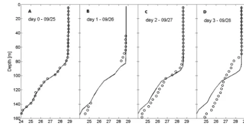
Figure 10. Comparison between Argo profile temperature

obser-vations (circles) and the 3DPWP model with the typhoon Hagupit setup (black solid line). Four plots are presented (A–D) showing a comparison between 19 September (A) and 22 September (D).

(Fig. 5), but the mixed layer temperature and salinity re-sponse to typhoon Jangmi (26–27 September) was weaker, most probably due to the float’s different relative position with respect to the typhoon track.

The wind stress coupling with inertial oscillations may also enhance the mixing on the right side of the typhoon track (Price, 1981), possibly helping to explain the results shown here. Observations taken during the passage of Jangmi, on the other hand, were limited to the left side of the typhoon track where mixing is not supported by coupling with iner-tial currents curl.

4 Modeling

4.1 Model – in situ comparison

In this section we present the control run results for HH and JJ simulations, and we compare the modeled ocean re-sponse with the available Argo float observations. For com-parison with in situ measurements, we use the results at the float location, which were, respectively, 40 km to the right of the track of typhoon Hagupit and 100 km to the left of the track of Jangmi. Figure 10 shows such profile comparisons for typhoon Hagupit. Overall, one can observe a very good correspondence between the observed and modeled cool-ing durcool-ing the early typhoon approach and passage of ty-phoon Hagupit for the four sequential Argo profiles plotted in Fig. 10. The maximum modeled cooling of 0.8◦_{C matches}

the observations quite well, for example, as do the tempera-ture tendencies within the mixed layer. The day-3 Argo pro-file in Fig. 10 is missing the upper 20 m of data, and there-fore it is not possible to compare it with modeled response, though modeled temperature below 20 m and depth of the thermocline are represented well when compared to obser-vations. It shows that model well reproduces cooling pro-cesses in this case. It is also apparent that temperature gra-dients within the upper thermocline are also well captured

29 1

2

Fig. 11. A comparison between the Argo profile temperature observations (circles) and the 3

3DPWP model with typhoon Jangmi set up (black solid line). Four plots are presented (A-D) 4

showing a comparison between September 25 (A) and September 28 (D). 5

6

Figure 11. A comparison between the Argo profile temperature

ob-servations (circles) and the 3DPWP model with typhoon Jangmi setup (black solid line). Four plots are presented (A–D) showing a comparison between 25 September (A) and 28 September (D).

by the model. Substantial deviation between model and ob-servations is evident far below the ML, and these may result from internal wave forcing from the model lateral bound-aries. During typhoon Hagupit passage, in situ observations were made within area of maximum modeled temperature anomaly. This comparison implies that 3DPWP model per-forms well within the area of the cold wake.

Figure 11 shows a comparison of the observed and mod-eled vertical profiles of temperature for typhoon Jangmi be-tween 25 and 28 September at a time when the float was approximately 100 km to the left of the storm track, in the opposite region from the right side maximum cooling pre-dicted by the model. As with Hagupit, it can be seen that the mixed layer temperature predicted by the model agrees well with the observed conditions. Although part of the day-1 in situ profile is missing above 40 m, one expects that it is well mixed and similar to the prior profile under strong wind conditions evident in Fig. 5. The model also does well in predicting the depth of the mixed layer particularly dur-ing days 1 and 2. Note that the observed cooldur-ing comes to an end on 27 September after the SSTs reach a minimum tem-perature of 28.6◦C. The model performs well in this regard with no change in temperature detected between days 2 and 3. The model on day 3 shows a relatively deeper MLD com-pared with the observations but that might be due to thermo-cline depth modified by the internal waves or other physical processes that were not represented in the model. Note that modeled profile has not changed from the previous day, when thermocline structure of observed profiles is clearly different. Since the typhoon at this time already passed by the float lo-cation, it is likely that the observed change is due to factors other than interaction with typhoon Jangmi. Model estimates of the MLD and temperature gradient within the thermocline are quite good with the exception of day 3.

Although typhoon Jangmi case has stronger winds, the modeled cold wake is weaker than for Hagupit. One pos-sible explanation may lie in the role of the initial ocean static stability and MLD in contributing to the overall wake

30 1

2

Fig. 12. Double-TC surface temperature anomaly (see EQ. 1). Here, the distance 3

perpendicular to the best track is plotted on the lower x-axis with negative values represent 4

the distance to the left of the track, and positive values the distance to the right of the track. 5

The upper x-axis present the same distance but normalized by the radius of maximum wind 6

which is 25 km in this case. Color scale represents temperature anomaly [C]. 7

8

Figure 12. Double-TC surface temperature anomaly (see Eq. 1).

Here, the distance perpendicular to the best track is plotted on the lowerxaxis with negative values representing the distance to the left of the track and positive values the distance to the right of the track. The upperxaxis presents the same distance but normalized by the radius of maximum wind, which is 25 km in this case. Color scale represents temperature anomaly [◦C].

cooling (Price, 1981). The data plotted in Fig. 6 show that the temperature at 100 m depth is about 27◦C for both of the initial profiles. However, comparing the temperature at 100 m to the SST in each case we find a 2.4◦C difference for the pre-Hagupit profile and 1.6◦C for the pre-Jangmi pro-file. The bigger temperature differences (less stable condi-tions) suggest that a higher cooling potential may exist in the Hagupit case. A shallower initial MLD causes a bigger cool-ing in the ocean for pre-Hagupit case in comparison to the pre-Jangmi case. In addition, presence of the barrier layer in pre-Jangmi profile is influencing the results: the pre-Jangmi salinity profile (squares at middle plot in Fig. 5) shows that, within the 80 m deep ML, there exists a shallower layer of fresher (∼0.1 psu) water, and such a structure may reduce the amount of cooling associated with the typhoon passage (Wang et al., 2011).

Another possible explanation for weaker ocean response to stronger typhoon Jangmi is counter-coupling with inertial currents forced on the upper ocean by typhoon Hagupit pas-sage. It is known (Price, 1981) that interaction between wind field curl and inertial motions is one of the key factors for inhomogeneous response of the upper ocean to typhoon-like forcing resulting in development of the cold wake to the right side of typhoon track (in the Northern Hemisphere). There-fore coupling with inertial oscillations that preexisted prior to the typhoon approach might either benefit or suppress mix-ing. We will address this point by the analysis of HHH ex-periments in the next section.

The overall comparisons with the Argo float indicate that the 3DPWP model does a good job in simulating the mixed-layer temperature and vertical structure changes during the individual typhoon passages. It can be used to investigate the ocean response to two sequential typhoon-like forcing.

31 1

2

Fig. 13. Vertical section of the double-TC temperature anomaly (see EQ. 1)averaged over an 3

inertial period (40h). The lower x-axis represents distance from the Jangmi track in km; the 4

upper x-axis is the same distance normalized by radius of maximum wind which is 25 km in 5

this case; the ordinate represents ocean depth in m. The 0 position is at the typhoon center. 6

Color scale represents temperature anomaly [C]. 7

8

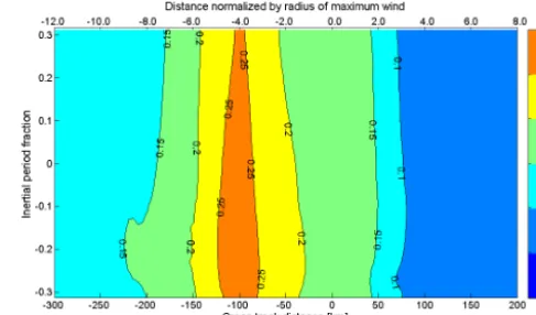
Figure 13. Vertical section of the double-TC temperature anomaly

(see Eq. 1) averaged over an inertial period (40 h). The lowerxaxis represents distance from the Jangmi track in kilometers; the upper xaxis is the same distance normalized by radius of maximum wind, which is 25 km in this case; the ordinate represents ocean depth in meters. The 0 position is at the typhoon center. Color scale repre-sents temperature anomaly [◦C].

4.2 Influence of typhoon Hagupit on typhoon Jangmi ocean response

The close proximity of the Hagupit and Jangmi tracks (140 km) and passage (6 days) over Argo float 5901579 raises a natural question: what influence did typhoon Hagupit have on the oceanic response caused by typhoon Jangmi? To investigate this relationship, we use the 3DPWP model to simulate the oceanic response caused by the typhoon Jangmi using the pre-Hagupit conditions as the typhoon’s initial state (HJ) and by Hagupit and Jangmi with a 6-day gap between them (HHJ). We should stress that the effects of typhoon Hagupit are not only limited to the vertical ocean mixing, but may also include changes in the freshwater flux due to pre-cipitation, inertial ocean motions, and other effects that may depend on a characteristic time of relaxation (Price et al., 2008). However, we concentrate here on contribution from the wind-driven forcing, and therefore shortwave flux and freshwater flux were set to 0 in this experiment. The initial oceanic state is a horizontally homogeneous ocean based on the Argo profile from 19 September.

To quantify the difference between these two experiments, let us define the double-TC anomaly difference as

T (t )= [THJ(t )−THJ(t=0)] − [THHJ(t )−THHJ(t=t1)], (1) where indices HJ and HHJ refer to “experiment 1” and “ex-periment 2” simulations respectively. Ocean state at timet1 is disturbed by typhoon Hagupit and represents upper ocean structure prior to the arrival of typhoon Jangmi.

It can be seen (Figs. 12 and 13) that cooling caused by typhoon Jangmi would have been significantly stronger if it had not been preceded by typhoon Hagupit. The cold wake behind Jangmi in the HJ run is situated on the right side of

the track and has a width of roughly 100 km. Figure 12 shows that temperature anomaly would be magnified but also on the opposite side. Strongest difference is visible 50–100 km to the left of the track of typhoon Jangmi where the cold wake of typhoon Hagupit is located. In HHJ run this part of the ocean was strongly disturbed by Hagupit; thus mixed layer was cooled and deepened. Additional cooling due to pas-sage of Jangmi was only 0.3◦C. If there were no Hagupit, downward momentum transport and mixing enhanced by ty-phoon Jangmi would have accounted for twice as strong mix-ing in this location. The different horizontal distributions of temperature anomaly simulated with the same atmospheric forcing suggest that disturbed and undisturbed ocean initial conditions, especially the initial MLD, influenced not only the amplitude of the anomaly but also its spatial distribution. Figure 13 presents the double-TC temperature anomaly verti-cal cross section averaged over an inertial period. Since a ty-phoon passage produces inertial oscillations in the ocean, we average the simulation results over 40 h period (roughly the period of inertial oscillations at 17.5◦N) to remove them. The abscissa in the plot represents the distance from the Jangmi track, and the ordinate represents the ocean depth. The or-dinate position is at the typhoon center. The surface cold anomaly is seen to be approximately 0.4◦C both to the right and left side of the track. Beneath the surface, there is an al-ternating positive and negative double-TC anomalies extend-ing across the typhoon track with a larger and more complex pattern on the left side of typhoon. This is due to a disturbed initial upper ocean on the left of Jangmi due to Hagupit. The subsurface net cooling down to about 50 m would have been stronger if there were no typhoon Hagupit.

A second question that can be examined is how the fi-nal ocean state after the passage of two sequential cyclones might differ from that obtained with the passage of just one typhoon. Let us introduce the following final-state tempera-ture anomaly:

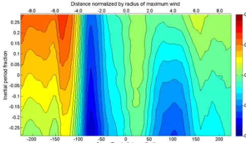
T (t )= [THJ(t )−THJ(t=0)] − [THHJ(t )−THHJ(t=0)], (2) where the first term defines the final ocean state after the pas-sage of Jangmi without any influence from Hagupit. The sec-ond term represents a sequence of oceanic anomalies caused by the passage of Hagupit followed by Jangmi in the sin-gle model run. Temperature defined in Eq. (2) is presented in Fig. 14. An overall effect on the ocean of two sequen-tial typhoons is stronger then the effect of typhoon Jangmi itself (indicated by positive values), though substantial vari-ation in temperature anomaly is visible. On the left side of Jangmi’s track the anomaly is stronger, which means that two collocated typhoons caused cooling of 0.25◦C stronger then Jangmi alone. This can be explained by the absence of Hagupit’s forcing on the ocean; note that −100 km is in the peak region of the Hagupit-induced cold wake. On the right side of typhoon Jangmi’s track, the joint effect of Hagupit and Jangmi is only 0.06◦C stronger then cooling from Jangmi alone – which is small. This accounts for only

32 1

2

Fig. 14. The HJ SST anomaly with respect to the total HHJ run anomaly (see EQ. 1). Here, 3

distance perpendicular to the best track is plotted on the lower x-axis; negative values are to 4

the left of the track, and positive values are to the right of the track. The upper x-axis present 5

the same distance but normalized by the radius of maximum wind which is 25 km in this case. 6

On the y-axis there is distance along the trajectory represented as time normalized by the 7

inertial oscillation period (40 h). The cross track distance measures distance from the 8

trajectory of typhoon Jangmi. The position of typhoon Hagupit is at -140 km. It can be seen 9

that there is positive anomaly to the left and negative anomaly to the right of Jangmi‘s track. 10

Color scale represents temperature anomaly [C]. 11

12

Figure 14. The HJ SST anomaly with respect to the total HHJ run

anomaly (see Eq. 1). Here, distance perpendicular to the best track is plotted on the lowerxaxis; negative values are to the left of the track, and positive values are to the right of the track. The upper xaxis presents the same distance but normalized by the radius of maximum wind, which is 25 km in this case. On theyaxis there is distance along the trajectory represented as time normalized by the inertial oscillation period (40 h). The cross-track distance measures distance from the trajectory of typhoon Jangmi. The position of ty-phoon Hagupit is at−140 km. It can be seen that there is positive anomaly to the left and negative anomaly to the right of Jangmi’s track. Color scale represents temperature anomaly [◦C].

5 % of temperature anomaly in the cold wake. Note that cool-ing reported in this study depends on momentum transfer and mixing exclusively. Factors like heavy precipitation, which is known to form barrier layers and therefore limit magnitude of anomaly (Wang et al., 2011), were omitted.

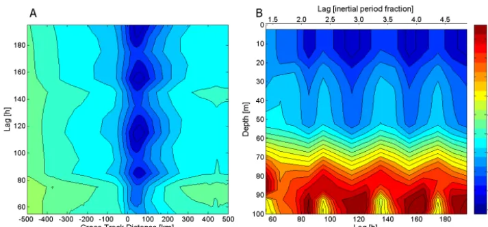
Up to now we discussed how the presence of typhoon Hagupit influences ocean response to typhoon Jangmi. The next set of numerical experiments is designed to answer the question about the role of distance between typhoon centers on strength of oceanic cooling effects. To simplify the prob-lem, we performed a series of simulations using two identical Hagupit-like wind fields following the same trajectory but with different time lags ranging from 55 to 195 h between them (HHH). Results (Fig. 15) are averaged over the inertial oscillation period. Panel A shows cross-track SST anomaly from different lags; an oscillation with period of∼40 h is visible in area of the maximum cooling (x=60 km) with magnitude of∼0.2◦C. The oscillation period agrees with the inertial oscillation period at this latitude. The first SST anomaly minimum of 0.1◦_{C is visible at 85 h lag. As in panel}

A, panel B shows the vertical cross section of temperature anomaly along the cold wake (x=60 km in panel A). One can notice the dependence of the temperature anomaly on lag time between sequential typhoons in the surface layer as well as below the thermocline. This is due to the coupling be-tween wind stress curl and inertial motions in the mixed layer (Price, 1981). The results show, for Hagupit-like typhoon, the wind stress curl and inertial motion coupling effect on the upper ocean temperature cooling occurred after two inertial

33 1

2

Fig. 15. The HHH run results. Panel A is SST anomaly. On x-axis is cross track distance in 3

km and on y-axis is lag between Hagupit like forcing in h. Panel B is vertical cross section 4

along cold wake (x=60 km on Panel A). On x-axis is lag between Hagupit like forcing in h 5

(lower x-axis) and as fraction of inertial period (upper x-axis). On y-axis is depth in m. Color 6

scale represents temperature anomaly [C]. Both panels use the same color scale. 7

Figure 15. The HHH run results. Panel (A) is SST anomaly. Onxaxis is cross-track distance in kilometers, and onyaxis is lag between Hagupit like forcing in h. Panel (B) is vertical cross section along cold wake (x=60 km in panel A). Onxaxis is lag between Hagupit like forcing in h (lowerxaxis) and as fraction of inertial period (upperxaxis). Onyaxis is depth in meters. Color scale represents temperature anomaly [◦C]. Both panels use the same color scale.

oscillations (80 h). The maximum surface cold anomaly is about 1.4◦C. It is interesting to note that typhoon Jangmi oc-curred approximately 5 days (120 h) after typhoon Hagupit, which is within the range of maximum anomaly seen from HHH experiments. This set of numerical experiments pro-vides some evidence of ocean response to sequential TC in terms of the inertial oscillation effect.

5 Summary and discussion

We consider the interaction of two typhoons closely collo-cated in time and space on the resulting observed and sim-ulated ocean cold wake structure. We show unique observa-tions of high-repetition Argo floats that collected in situ ob-servations in close proximity to both typhoons. The numer-ical model was validated by imposing realistic atmospheric forcing using satellite-derived (CIRA) winds and observed cyclone tracks, and compared model results with observed ocean structure using the high-repetition Argo float. We show that cooling caused by the second typhoon (typhoon Jangmi) would have been about 0.5◦C (30 %) stronger if it had not been preceded by typhoon Hagupit. Additionally we also see a different spatial distribution with stronger negative SST anomalies in both cold wake region and on the left side of the track. Similar to previous studies, our results confirm the importance of initial ocean condition on the ocean response to typhoon forcing. The disturbed ocean conditions set up by a previous typhoon such as the case studied here deepen the mixed-layer depth and weaken the ocean response for the second typhoon following a similar track. This, in turn, may produce a stronger second typhoon due to less ocean cooling. We show that the amount of pre-storm upper-ocean kinetic energy in the ocean is as important as the pre-storm mixed layer depth to affect the magnitude of the ocean cooling dur-ing the storm stage. Finally, we show that the magnitude of

the cooling may also depend on the time lag between suc-cessive typhoons. Results suggest that the magnitude of the anomaly oscillates with the period of the inertial current and that the first maximum cooling occurs after two inertial os-cillation periods (80 h).

We present model simulations of two typhoons’ impact on the upper ocean and their possible intricate relationship driven by both undisturbed and disturbed initial oceanic ther-modynamical and dynamical states. This paper indicates that studies of successive ocean–atmosphere tropical cyclone in-teraction will benefit from more high-repetition Argo float measurements such as these reported here and from a higher density network of such floats. More coupled model studies are also warranted in order to further understand the impact of the ocean processes discussed here on typhoon’s track and intensity change.

Copyright statement

This work relates to Department of the Navy Grant N62909-11-1-7061 issued by Office of Naval Research Global. The United States Government has a royalty-free license through-out the world in all copyrightable material contained herein.

Acknowledgements. This research was sponsored by the Naval

Research Laboratory under Program Element 0601153N. D. B. Baranowski was supported by the ONR grant (award number N00014-10-1-0898) and ONR Global NICOP (award number N62909-11-1-7061). The Japan Meteorological Agency best track data can be found at http://www.jma.go.jp/jma/jma-eng/ jma-center/rsmc-hp-pub-eg/besttrack.html. We would like to thank Dean Roemmich and John Gilson for providing gridded Argo data used here for deriving climatology as well as answering many questions on Argo data as well as their hospitality during D. B. Baranowski’s stays at Scripps Institution of Oceanography.

D. B. Baranowski would like to extend his gratitude to Hiroyuki Yamada for his help during the R/V Mirai cruise in summer of 2010 and hands-on experience with the high-repetition Argo floats. John Knaff and Mark deMaria provided us with CIRA wind data. We would like to thank Jim Price for providing the 3DPWD code, and James Ridout and Jerome Schmidt for proofreading this paper.

Edited by: E. J. M. Delhez

References

Babin, S. M., Carton, J. A., Dickey, T. D., and Wiggert, J. D.: Satellite evidence of hurricane-induced phytoplankton blooms in an oceanic desert, J. Geophys. Res.-Oceans, 109, C03043, doi:10.1029/2003jc001938, 2004.

Black, P. G., D’Asaro, E. A., Drennan, W. M., French, J. R., Niiler, P. P., Sanford, T. B., Terrill, E. J., Walsh, E. J., and Zhang, J. A.: Air-sea exchange in hurricanes – Synthesis of observations from the coupled boundary layer air-sea transfer experiment, Bull. Am. Meteorol. Soc., 88, 357–374, doi:10.1175/bams-88-3-357, 2007.

Brand, S.: The Effects on a Tropical Cyclone of Cooler Surface Wa-ters Due to Upwelling and Mixing Produced by a Prior Tropi-cal Cyclone, J. Appl. Meteorol., 10, 865–874, doi:10.1175/1520-0450(1971)010<0865:teoatc>2.0.co;2, 1971.

Cione, J. J. and Uhlhorn, E. W.: Sea surface temperature variabil-ity in hurricanes: Implications with respect to intensvariabil-ity change, Mon. Weather Rev., 131, 1783–1796, 2003.

D’Asaro, E. A., Sanford, T. B., Niiler, P. P., and Terrill, E. J.: Cold wake of Hurricane Frances, Geophys. Res. Lett., 34, L15609, doi:10.1029/2007gl030160, 2007.

D’Asaro, E. A., Black, P., Centurioni, L., Harr, P., Jayne, S., Lin, II, Lee, C., Morzel, J., Mrvaljevic, R., Niiler, P. P., Rainville, L., Sanford, T., and Tang, T. Y.: Typhoon-Ocean Interaction in the Western North Pacific: Part 1, Oceanography, 24, 24–31, 2011. Elsberry, R. L. and Harr, P. A.: Tropical Cyclone Structure (TCS08)

Field Experiment Science Basis, Observational Platforms, and Strategy, Asia-Pac., J. Atmos. Sci., 44, 209–231, 2008.

Emanuel, K., DesAutels, C., Holloway, C., and Korty, R.: Environ-mental control of tropical cyclone intensity, J. Atmos. Sci., 61, 843–858, 2004.

Falkovich, A. I., Khain, A. P., and Ginis, I.: Motion and Evolution of Binary Tropical Cyclones in a Coupled Atmosphere–Ocean Numerical Model, Mon. Weather Rev., 123, 1345–1363, doi:10.1175/1520-0493(1995)123<1345:maeobt>2.0.co;2, 1995.

Firing, E., Lien, R. C., and Muller, P.: Observations of strong inertial oscillations after the passage of tropical cyclone Ofa, J. Geophys. Res.-Oceans, 102, 3317–3322, 1997.

Fisher, E. L.: Hurricanes and the Sea-Surface Temperature Field, J. Meteorol., 15, 328–331, 1958.

Frank, W. M. and Young, G. S.: The interannual variability of tropical cyclones, Mon. Weather Rev., 135, 3587–3598, doi:10.1175/mwr3435.1, 2007.

Hong, X. D., Chang, S. W., and Raman, S.: Modification of the loop current warm core eddy by Hurricane Gilbert (1988), Nat. Hazards, 41, 501–514, doi:10.1007/s11069-006-9057-2, 2007.

Jacob, S. D. and Koblinsky, C. J.: Effects of precipitation on the upper-ocean response to a hurricane, Mon. Weather Rev., 135, 2207–2225, doi:10.1175/mwr3366.1, 2007.

Lander, M. A.: An Exploratory Analysis of the Relationship be-tween Tropical Storm Formation in the Western North Pacific and Enso, Mon. Weather Rev., 122, 636–651, 1994.

Lin, I., Liu, W. T., Wu, C. C., Wong, G. T. F., Hu, C. M., Chen, Z. Q., Liang, W. D., Yang, Y., and Liu, K. K.: New evidence for en-hanced ocean primary production triggered by tropical cyclone, Geophys. Res. Lett., 30, 1718, doi:10.1029/2003gl017141, 2003. Mrvaljevic, R. K., Black, P. G., Centurioni, L. R., Chang, Y.-T., D’Asaro, E. A., Jayne, S. R., Lee, C. M., Lien, R.-C., Lin, I. I., Morzel, J., Niiler, P. P., Rainville, L., and Sanford, T. B.: Ob-servations of the cold wake of Typhoon Fanapi (2010), Geophys. Res. Lett., 316–321, doi:10.1002/grl.50096, online first, 2013. Powell, M. D., Vickery, P. J., and Reinhold, T. A.: Reduced drag

co-efficient for high wind speeds in tropical cyclones, Nature, 422, 279–283, doi:10.1038/Nature01481, 2003.

Price, J. F., Morzel, J., and Niiler, P. P.: Warming of SST in the cool wake of a moving hurricane, J. Geophys. Res.-Oceans, 113, C07010, doi:10.1029/2007jc004393, 2008.

Price, J. F.: Upper Ocean Response to a Hurricane, J. Phys. Oceanogr., 11, 153–175, 1981.

Price, J. F., Weller, R. A., and Pinkel, R.: Diurnal Cycling – Ob-servations and Models of the Upper Ocean Response to Diurnal Heating, Cooling, and Wind Mixing, J. Geophys. Res.-Oceans, 91, 8411–8427, 1986.

Price, J. F., Sanford, T. B., and Forristall, G. Z.: Forced Stage Re-sponse to a Moving Hurricane, J. Phys. Oceanogr., 24, 233–260, 1994.

Price, J. F.: Metrics of hurricane-ocean interaction: vertically-integrated or vertically-averaged ocean temperature?, Ocean Sci., 5, 351–368, doi:10.5194/os-5-351-2009, 2009.

Ramage, C. S.: Typhoons of October 1970 in South China Sea – Intensification, Decay and Ocean Interaction, J. Appl. Meteorol., 13, 739–751, doi:10.1175/1520-0450, 1974.

Roemmich, D. and Gilson, J.: The 2004-2008 mean and annual cycle of temperature, salinity, and steric height in the global ocean from the Argo Program, Prog. Oceanogr., 82, 81–100, doi:10.1016/j.pocean.2009.03.004, 2009.

Sanford, T. B., Price, J. F., and Girton, J. B.: Upper-Ocean Response to Hurricane Frances (2004) Observed by Profil-ing EM-APEX Floats, J. Phys. Oceanogr., 41, 1041–1056, doi:10.1175/2010jpo4313.1, 2011.

Schade, L. R. and Emanuel, K. A.: The ocean’s effect on the intensity of tropical cyclones: Results from a simple cou-pled atmosphere-ocean model, J. Atmos. Sci., 56, 642–651, doi:10.1175/1520-0469(1999)056<0642:TOSEOT>2.0.CO;2, 1999.

Uhlhorn, E. W. and Shay, L. K.: Loop Current Mixed Layer Energy Response to Hurricane Lili (2002), Part I: Observations, J. Phys. Oceanogr., 42, 400–419, doi:10.1175/jpo-d-11-096.1, 2011. Uhlhorn, E. W. and Shay, L. K.: Loop Current Mixed Layer

Energy Response to Hurricane Lili (2002), Part II: Idealized Numerical Simulations, J. Phys. Oceanogr., 43, 1173–1192, doi:10.1175/jpo-d-12-0203.1, 2013.

Wada, A. and Usui, N.: Importance of tropical cyclone heat potential for tropical cyclone intensity and intensification