SRef-ID: 1607-7946/npg/2004-11-589
Nonlinear Processes
in Geophysics
© European Geosciences Union 2004
Soil nutrient cycles as a nonlinear dynamical system
S. Manzoni1, A. Porporato1, P. D’Odorico2, F. Laio3, and I. Rodriguez-Iturbe4
1Department of Civil and Environmental Engineering, Duke University, 127 Hudson Hall, Durham, NC 27708, USA 2Department of Environmental Sciences, University of Virginia, 291 McCormick Road, Charlottesville, VA 22904, USA 3Dept. di Idraulica Trasporti e Infrastrutture Civili, Politecnico di Torino, Corso Duca degli Abruzzi 24, 10129 Torino, Italy 4Department of Civil and Environmental Engineering, Princeton University, Olden Street, Princeton, NJ 08544, USA
Received: 2 July 2004 – Revised: 7 October 2004 – Accepted: 12 October 2004 – Published: 24 November 2004 Part of Special Issue “Nonlinear deterministic dynamics in hydrologic systems: present activities and future challenges”
Abstract. An analytical model for the soil carbon and ni-trogen cycles is studied from the dynamical system point of view. Its main nonlinearities and feedbacks are analyzed by considering the steady state solution under deterministic climatic conditions. It is shown that, changing hydro-climatic conditions, the system undergoes dynamical bifur-cations, shifting from a stable focus to a stable node and back to a stable focus when going from dry, to well-watered, and then to saturated conditions, respectively. An alternative de-generate solution is also found in cases when the system can not sustain decomposition under steady external conditions. Different basins of attraction for “normal” and “degenerate” solutions are investigated as a function of the system initial conditions. Although preliminary and limited to the specific form of the model, the present analysis points out the impor-tance of nonlinear dynamics in the soil nutrient cycles and their possible complex response to hydro-climatic forcing.
1 Introduction
Soil biogeochemical cycles are characterized by complex dy-namics, acting at different spatial and temporal scales. They are impacted by vegetation and hydro-meteorological forcing and, in turn, exert various feedbacks on the ecosystems, at-mosphere, and climate dynamics. Various models have been proposed in the past to investigate these dynamics (e.g. Par-ton et al., 1988; Hunt et al., 1991; Gusman and Marino, 1999; Melillo et al., 1995; Benbi and Richter, 2002; Schimel and Weintraub, 2003; Schimel and Bennett, 2004, and references therein) resulting in a deeper understanding of soil biogeo-chemistry under a broad variety of climatic and ecological conditions.
However, given the difficulty of modeling the biolog-ical components and the high variability of the hydro-meteorological forcing, our ability to model and predict soil Correspondence to: A. Porporato
nutrient dynamics is still incomplete. The lack of knowl-edge in certain areas is coupled with a strong dependence of simulation results on the model conceptual and mathematical structure (Melillo et al., 1995). This is clear from the fact that simulations using different models present increasing incon-sistencies when the time scale of interest is increased, show-ing the difficulty in predictshow-ing the long-term impact of differ-ent hydro-climatic regimes on the soil nutridiffer-ent cycles.
The hydro-climatic variability regulates the sequence of fluxes between different components of soil nutrient cycles and determines the temporal dynamics of the system state variables at different time scales. In particular, the soil mois-ture and temperamois-ture regimes control decomposition, leach-ing, and plant uptake and, indirectly, influence vegetation growth and composition of plant residues. Previous theo-retical investigations focused mostly on the linear analyses of soil nutrient cycles, providing useful assessments of the effects of model parameters on ecosystem processes (e.g. Bolker et al., 1998; Katterer and Andr`en, 2001; Baisden and Amundson, 2003). However, very little attention has been devoted to the nonlinear dynamics of soil nutrient cycles. To this regard, the techniques developed in dynamical system theory (e.g. stability and bifurcation analysis) can be applied to simple mathematical models of soil nutrient cycles to ob-tain a general description of the system internal dynamics and its response to external perturbations.
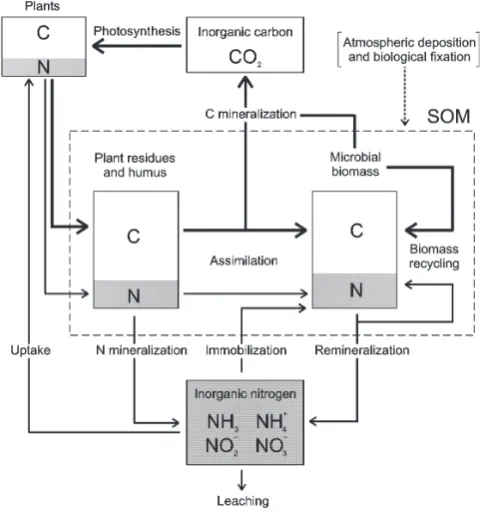
Fig. 1. Schematic representation of the soil carbon and nitrogen
cy-cles, with particular attention to the interactions among the three main components of the SOM: plant litter, humus and biomass. Thick lines: C fluxes; thin lines: N fluxes. Modified after Mary et al. (1996).
and the model presentation, we will analyze the system equi-librium conditions and the modalities of approach to equilib-rium.
2 Nonlinearities and feedbacks in the C and N cycles in soils
The carbon cycle in the soil-plant system is dominated by a sequence of biochemical processes including assimilation (photosynthesis), residues production and deposition, and decomposition (litter mineralization), which releases carbon as CO2back to the atmosphere (Fig. 1). Assuming a
long-term equilibrium condition of ecosystems, the total respi-ration is generally balanced by the input of plant residues, while at shorter time scales (e.g. seasonal-to-interannual) the carbon content is subject to fluctuations induced by hydro-climatic and other environmental forcing.
As shown in Fig. 1, the carbon is stored in the soil or-ganic matter (SOM), which is a complex and varied mixture of organic substances, with three main components: plant residues, microbial biomass, and humus. Plant residues ac-cumulate on the soil surface where they are degraded by both physical and biological agents. The organic compounds are then partially assimilated and partially oxidated by the mi-crobial biomass in the soil. The biomass provides a high turnover rate of C and N in the SOM pool, with release of
stable mineralized products of the catabolic processes (e.g. CO2) at each turnover (Molina and Smith, 1998).
The carbon assimilation and respiration processes are af-fected by the composition of organic compounds and by cli-matic conditions. The presence of water and elevated soil temperatures are key factors to provide a fast decomposition and biomass growth. The relation between biomass activ-ity and soil water content is strongly non-linear (Brady and Weil, 1996), since both lack and excess of water are limiting. In particular, at low soil moisture levels the reduced diffu-sion of nutrients limits their availability to microbes, while low soil water potentials reduce hydration and enzymatic ac-tivity of microbes causing water stress. Interestingly, the water stress of soil microbes has similar characteristics to plant water stress (Porporato et al., 2001). The dependence of decomposition on soil temperature is also nonlinear, rais-ing from zero at low temperatures (∼ −5◦C) to a maximum at around 40◦C (although these values tend to be site specific) (Ratkowsky et al., 1982; Gusman and Marino, 1999; Benbi and Richter, 2002). When the conditions are favorable, ni-trification is quite rapid. As a result, in hot and dry environ-ments, sudden water availability can cause a flush of soil ni-trate production (D’Odorico et al., 2003), which may greatly influence the growth patterns of natural vegetation (Cui and Caldwell, 1991; Fierer and Schimel, 2002).
A second important form of nonlinearity is related to the Mineralization-Immobilization Turnover (MIT) and the C/N ratio of microbial biomass. In fact, in order to main-tain a constant C/N ratio during its growth, the microbial biomass needs to assimilate proportional amounts of carbon and nitrogen, independently of the composition of the or-ganic compounds of the substrate (Brady and Weil, 1996). As a consequence, if the nitrogen content of the decomposed compounds is high, mineralization proceeds unrestricted and mineral components in excess are released into the soil, while if such compounds are nitrogen poor, the microbes immobi-lize mineral nitrogen for their growth (Fig. 1). If mineral ni-trogen is not available, immobilization is halted (Jansson and Persson, 1982; Mary et al., 1996; Benbi and Richter, 2002). The MIT is thus characterized by an extremely strong non-linearity that acts as a threshold-process. As will be seen in Sect. 3.1, its triggering is governed by a subtle interaction between nutrient dynamics and environmental conditions. It must be noted, however, that in field conditions this sharp nonlinearity may be somewhat smoothed out by the presence of different types of decomposing bacteria and fungi with different C/N ratios.
3 Model structure
Porporato et al. (2003) developed a simplified model of the nutrient cycle valid at the daily time scale and considering vertically-averaged values of carbon and nitrogen concentra-tions over the active soil depth, Zr. Here we only give a
brief description of the model and refer to Porporato et al. (2003) for details. The only external input of carbon and ni-trogen to the system is through vegetation litter. Respiration is the only carbon output, while the nitrogen losses are leach-ing and plant uptake. Fluxes such as ammonium adsorption and desorption, deposition and volatilization are neglected, being of lesser importance for the soil C-N balances at the daily-to-seasonal time scale (Mary et al., 1996; Baisden and Amundson, 2003; D’Odorico et al., 2003).
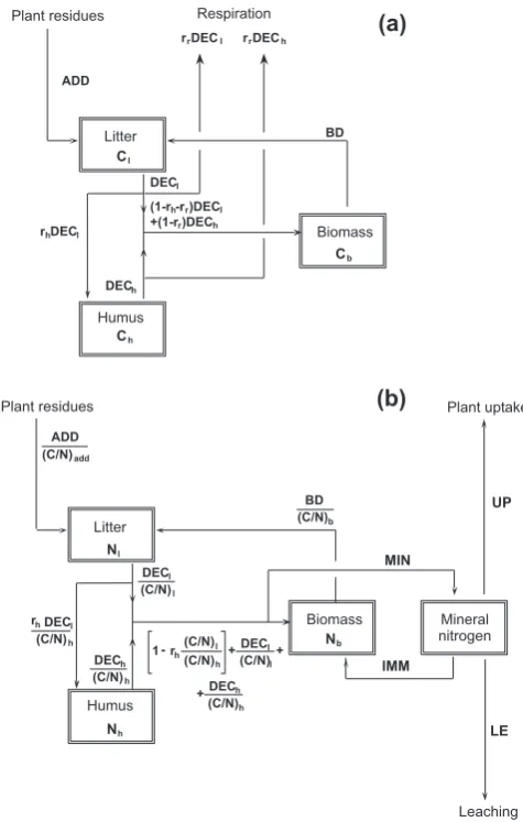
The carbon and nitrogen cycles are modeled using four different pools, one for each main component of the system (Fig. 2). SOM is divided into three compartments, repre-senting litter, humus, and microbial biomass. The general structure is in agreement with the recommendation of Bolker et al. (1998), who suggested using at least a fast and a slow decomposing pool to model SOM. Moreover, according to Baisden and Amundson (2003), the explicit description of the biomass dynamics can only be avoided when one is in-terested in the long-term dynamics. For simplicity, ammo-nium and nitrate are lumped into a single pool for mineral nitrogen. The nitrogen pools are defined through their C/N ratios as in Bolker et al. (1998), Mueller et al. (1998) and in Katterer and Andr`en (2001).
Once plant residues enter the litter pool, they move partially to humus and partially to the biomass pool, losing a respired fraction during the decomposition process (Molina and Smith, 1998). Differently from the CENTURY model (Bolker et al., 1998), decomposition is explicitly modeled to account for the fact that it also depends on the amount of biomass, in agreement with Schimel and Weintraub (2003). The model needs seven state variables, each in terms of mass per unit volume of soil (e.g. g m−3), six of them to describe carbon and nitrogen concentrations in the three SOM pools, one for the soil mineral nitrogen (see the scheme in Fig. 2): Cl, carbon concentration in the litter pool;
Ch, carbon concentration in the humus pool;
Cb, carbon concentration in the biomass pool;
Nl, organic nitrogen concentration in the litter pool;
Nh, organic nitrogen concentration in the humus pool;
Nb, organic nitrogen concentration in the biomass pool;
N, mineral nitrogen concentration in the soil.
The temporal dynamics of such variables is controlled by a system of seven coupled differential equations that describe the balance of carbon and nitrogen in the various pools and the fluxes among them, in terms of mass per unit volume per unit time (e.g. g m−3d−1). Since many of the fluxes are con-trolled by environmental fluctuations, their modeling explic-itly accounts for soil moisture and temperature conditions.
Fig. 2. Schematic representation of the main components of the
model. (a) Soil carbon cycle; (b) soil nitrogen cycle. After Porpo-rato et al. (2003).
The system of first order nonlinear differential equations is (Fig. 2)
dCl
dt =ADD+BD−DECl (1)
dNl
dt =
ADD (C/N)add
+ BD
(C/N)b
− DECl (C/N)l
(2) dCh
dt =rhDECl−DECh (3)
dNh
dt =rh DECl
(C/N)h
− DECh (C/N)h
(4) dCb
dt =(1−rh−rr)DECl+(1−rr)DECh−BD (5) dNb
dt =
1−rh
(C/N)l
(C/N)h
DECl
(C/N)l
+
+DECh (C/N)h
− BD
(C/N)b
dN
dt =8−LE−U P . (7)
The first six equations represent the balances of litter (l subscript), humus (h subscript) and biomass (b subscript) pools, while the last one is the balance equation for the min-eral nitrogen, N. A brief description of the terms is given next. For a more detailed discussion of the rationale and modeling assumptions reference is made to Porporato et al. (2003).
The termADDis the external input into the system, rep-resenting the rate at which carbon in plant residues is added into the soil and made available to the microbial colonies. Here ADD is assumed to be constant in time. The term BDis the rate at which carbon returns to the litter pool due to the death of microbial biomass. Porporato et al. (2003) simply used a linear dependence on the amount of microbial biomass, i.e.BD=kdCb.
DECl represents the carbon output due to microbial
de-composition, modeled using a first order kinetics with respect to the carbon concentration in the litter pool,Cl(e.g. Hansen
et al. (1995); Gusman and Marino (1999); Birkinshaw and Ewen (2000)), as well as to the carbon in the biomass pool, Cb,
DECl = [ϕklf (s, T )Cb]Cl, (8)
where the coefficientϕis a non-dimensional factor account-ing for a possible reduction of the decomposition rate when the litter is very poor in nitrogen and immobilization is not sufficient to integrate the nitrogen required by bacteria (see Sect. 3.1). The constantkldefines the rate of decomposition
for the litter pool as a weighted average of the decomposition rates of the different organic compounds in the plant residues. Its average value is usually much higher than the correspond-ing value for humus,kh. The close relation of the
decompo-sition rate with the microbial biomass is due to the role of exoenzymes in the depolymerization process (Schimel and Weintraub, 2003; Schimel and Bennett, 2004).
The factorf (s, T ) =fd(s)ft(T )is of particular interest
here as it describes soil moisture (s) and soil temperature (T) effects on decomposition. Following Cabon et al. (1991) and Gusman and Marino (1999), the soil moisture control on aer-obic microbial activity and decomposition is modeled via a linear increase fromsbup to field capacity,s=sf cand a
hy-perbolic decrease from there to soil saturation (s =1). The parametersbrepresents a sort of permanent “wilting” point
for soil microbial biomass. Although this parameter is either not considered explicitly (Gusman and Marino, 1999; Porpo-rato et al., 2003) or assumed to be equal to the corresponding plant wilting point (Hunt et al., 1991), its role in soil nutri-ent dynamics is very important. In particular, its relation-ship with the plant wilting point,sw, that defines the level at
which transpiration and passive nitrogen uptake are stopped, provides a way to account for the impact of water stress on the competition for nutrients between plants and soil micro-bial biomass (Kaye and Hart, 1997). In terms of soil water potential, sb corresponds to a range between−0.8 and−8
MPa, depending on biomass composition; specifically, bac-teria show a higher sensitivity than fungi to water potential (e.g. Freckman, 1986). The corresponding values in terms of soil water content depend on soil type and are easily obtain-able through the so-called water retention curves (e.g. Laio et al., 2001).
The dependence of microbial activity on soil temperature is described by a quadratic relation (Ratkowsky et al., 1982; Katterer and Andr`en, 2001), with a minimum survival tem-perature for microbial biomass (about −5◦C, according to Hunt et al., 1991; Katterer and Andr`en, 2001) and an opti-mum temperature that, on account of the adaptation of micro-bial colonies to a specific site, can be taken as the maximum soil temperature measured in the field (Katterer and Andr`en, 2001). The inclusion offt(T )andsbare elements of novelty
with respect to the previous version of the model (Porporato et al., 2003).
The second equation of the system (Eq. 2) represents the nitrogen balance in the litter pool. This is similar to that of carbon, with each term divided by the C/N ratio of its respective pool. (C/N)add is the C/N ratio of added plant
residues, whose variability can produce pronounced changes in the C/N ratio of the litter pool and on the MIT turnover.
The balance equation for carbon in the humus pool (Eq. 3) has a single input flux, represented by the fractionrhof the
decomposed litter undergoing humification. It is also as-sumed that the products of the humification process from lit-ter have the same characlit-teristics, and thus the same C/N ra-tio, as the soil humus. As a consequence, the value of(C/N)h
remains constant in time so thatNh=(CC/Nh)
h.
The input of carbon in the biomass pool is represented by the fraction of organic matter incorporated by the microor-ganisms from litter and humus decomposition (see Fig. 2). The constantrr (0 ≤ rr ≤ 1−rh) defines the fraction of
decomposed organic carbon that goes into respiration, usu-ally estimated to be in the interval 0.6–0.8 (Brady and Weil, 1996). As for the biomass nitrogen balance, Eq. (6) has an additional term due to the net mineralization,8, whose mod-eling is described in Sect. 3.1.(C/N)bis assumed to be
con-stant, so that the sixth equation of the system (Eq. 6) can be written as Nb = (CC/Nb)
b. The constancy of (C/N)b
deter-mines the net mineralization8(see Sect. 3.1).
The last equation (Eq. 7) describes the balance of mineral nitrogen, in which mineralization is the only input, while plant uptake and leaching are the two losses. The latter is simply modeled as proportional to the deep infiltrationL(s) losses through a solubility coefficient a (Porporato et al., 2003),
LE=a L(s) s nZr
N , (9)
transpiration rate,Tp(s), and to the nitrogen concentration in
the soil solution, i.e. U Pp =a
Tp(s)
s nZr
N, (10)
where Tp(s) is characterized by two different regimes: a
stressed one with a linear increase of Tp(s) from 0 at sw
toTp,max ats∗, the level at which the plants begin to close
their stomata, and an unstressed one with a constant maxi-mum transpiration rateTp,maxfors > s∗(Laio et al., 2001).
Plants try to compensate the nitrogen deficit with the active mechanism of uptake only if the passive uptake is lower than a given plant demand, DEM. Following Porporato et al. (2003), when the diffusion of nitrogen ions into the soil is limiting, the active uptake is assumed to be proportional to the nitrogen concentration in the soil through a diffusion co-efficient,ku(in this case theNdemand can not be satisfied),
otherwise active uptake is simply the difference between the demand and the passive component.
3.1 Mineralization-immobilization dynamics
As mentioned before, the MIT is characterized by strongly nonlinear dynamics. Following Porporato et al. (2003), it is assumed that when the average C/N ratio of the biomass is lower than the value required by the microbial biomass, the decomposition results in a surplus of nitrogen, which is not incorporated by the bacteria, and net mineralization takes place. In contrast, if the decomposing organic matter is nitro-gen poor, bacteria try to meet their nitronitro-gen requirement by increasing the immobilization rate from ammonium and trate, thus depleting the mineral nitrogen pool. When the ni-trogen supply from immobilization is not sufficient to ensure a constant C/N ratio for the biomass, the rates of decompo-sitions are reduced below their potential values by means of the parameterϕ(e.g. see Eq. 8). Since the net fluxes among the various pools are important to the nitrogen balance, only the net amounts of mineralization and immobilization need to be modeled. This can be done as if they were mutually exclusive processes (Porporato et al., 2003). Thus, the net mineralization rate,8, is defined as
8=MI N−I MM. (11)
The switch between the two states takes place in order to maintain(C/N)b constant. Such a condition is determined
by the carbon and nitrogen balances for the biomass pool, as 8=DECh
1
(C/N)h
− 1−rr (C/N)b
+DECl
1
(C/N)l
− rh (C/N)h
−1−rh−rr (C/N )b
=
=ϕ f (s, T )Cb
khCh
1
(C/N)h
− 1−rr (C/N)b
+klCl
1
(C/N)l
− rh (C/N)h
−1−rh−rr (C/N)b
. (12)
When the term in curly brackets of Eq. (12) is positive, net mineralization takes place, while no net immobilization occurs. In such conditions, humus and litter decomposition proceed unrestricted and the parameterϕis equal to 1. In the opposite case, when the term in curly brackets of Eq. (12) is negative, net mineralization is halted and immobilization sets in. If the amount of mineral nitrogen is sufficient to sus-tain the biomass growth, immobilization occurs at a potential rate,I MMpot. In this caseϕis still equal to one. During
im-mobilization, nitrogen in the mineral pool is depleted, so that its concentration can become a limiting factor. As a conse-quence, an upper bound for immobilization, dependent onN as well as on the climatic forcing, can be defined as
I MMmax=kiNf (s, T )Cb. (13)
This upper bound for immobilization determines the con-dition
I MM =min{I MMpot, I MMmax} (14)
that yields a proper definition of ϕ (see Porporato et al. (2003) for details). The coefficientϕimpacts the decomposi-tion rates, and consequently the assimiladecomposi-tion rates, providing a relationship between the SOM dynamics and the mineral nitrogen availability.
The change of the sign of8, that controls MIT, depends mostly on the carbon to nitrogen ratio of the litter pool (C/N)l, since(C/N)h and(C/N)b are almost constant in a
particular site. As noted before, however, the simultaneous presence of different organisms in the decomposing commu-nity (e.g. bacteria, fungi, etc.), or shifts in its composition, may affect the net mineralization rate in a more complex way.
4 Steady state solution
In this section we carry out a deterministic analysis of the C-N model defined before. To this aim, soil moisture and temperature are assumed to remain constant, thus focusing on the intrinsic system behavior independently of the hydro-climatic variability.
In steady state conditions, the SOM carbon and nitrogen concentrations can be analytically determined from the full system (Eqs. 1–7) as
Cl,eq =
kd
ϕklf (s, T )[1−rr(1+rh)]
, (15)
Nl,eq = ADD (C/N)add +kd
Cb,eq
(C/N)b klf (s, T )Cb,eq
, (16)
Ch,eq =
rhklCl,eq
kh
, (17)
Cb,eq =
ADD
kd
h
1
ϕ(1−rr(1+rh))−1
i. (18)
The steady solutions for humus and biomass nitrogen,Nh
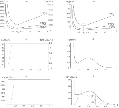
Fig. 3. Steady state solutions as a function of average soil moisture: (a)ClandCh; (b)Nl; (c)Cband litter decomposition,DECl; (d)N;
(e) mineralization,8; (f) passive,U Pp, active,U Pa, and total uptake,U P. Dashed lines refer to the steady state solution obtained with a functionADD(s)linearly decreasing withsunder wilting point.
carbon, according to their C/N ratios. Fig. 3 shows that, at the steady state,Cbis the only state variable which is
inde-pendent of the climate forcing, while the other SOM pools accumulate carbon and nitrogen when the decomposition ef-ficiency is low and lose them when the decomposition effi-ciency is high (i.e. near field capacity) and under elevated soil temperature conditions (see Sect. 3).
Equations (8) and (12) yield the steady state fluxes, where ϕis equal to one, being net mineralization a necessary con-dition for the steady state,
DECl,eq =
ADD
rr(1+rh)
, (19)
8eq=
ADD (C/N)add
. (20)
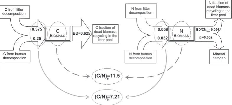
Equations (19) and (20) show that the carbon and nitrogen fluxes at steady state are independent of the climatic forc-ing. The specific values shown in Fig. 3 are obtained us-ing parameters estimated for a warm South African Savanna (D’Odorico et al., 2003). With such values, the ratio between
total carbon and nitrogen incoming in the biomass pool is lower than the(C/N)b, so that there is an excess of
nitro-gen, which results in net mineralization (Fig. 4). Mineraliza-tion is also inversely proporMineraliza-tional to(C/N)add since a poor
quality of the added litter decreases the amount of nitrogen entering in the biomass pool, thus limiting the surplus going to the mineral nitrogen pool and the nutrient availability for plants. This may affect the C/N ratio in the leaves, deter-mining a positive feedback for nitrogen limitation (Vitousek and Howarth, 1997). Moreover, high values of(C/N)addalso
decrease the quality of the litter, (C/N)l (Fig. 5), since the
biomass needs to maintain its C/N ratio by fixing N in its tis-sues. On the other hand, organic N is recycled in the system through the microbial biomass turnover, causing a nonlinear decrease of litter quality with increasing(C/N)add (Fig. 5).
As a consequence, a high N demand by microbial biomass (i.e. lower(C/N)b) increases the nitrogen content of the
lit-ter pool (Fig. 2), because of higher N turnover.
Fig. 4. Nitrogen and carbon balances for the biomass pool, in steady state conditions. The incoming C/N ratio is lower than(C/N)b, resulting in net mineralization. Fluxes are expressed in terms of g m−3d−1.
mineral nitrogen depends only on s through plant uptake (Fig. 3f) and leaching losses, the balance of which (Eq. 7) determines a local minimum and a local maximum (Fig. 3d). Apart from very low soil moisture values, the mineral nitro-gen can not accumulate in the soil due to plant uptake and leaching. Under nitrogen-limited conditions, such as those typical of the Nylsvley Savanna (Scholes and Walker, 1993; Vitousek and Howarth, 1997), plant nutrient demand (DEM) is not satisfied at steady state and consequently the plant up-take remains directly dependent on the N content in the soil (Porporato et al., 2003).
4.1 Approach to equilibrium and stability analysis
Figure 6 shows the dynamics of carbon biomass towards equilibrium as a function of soil moisture and under constant temperature condition. The trajectories are obtained by nu-merically integrating the balance equation system (Eqs. 1–7) using a standard ordinary differential equation solver. For soil moisture below the ’wilting’ points < sb,
decompo-sition is not sustained and equilibrium is degenerate (see Sect. 4.2 for details). For soil moisture that are above the wilting point, but low compared to field capacity, microbial activity is low. Following the usual classification of the dif-ferent equilibrium points of dynamical systems (e.g. Argyris et al., 1994), the equilibrium is a stable focus with damped oscillation to equilibrium. If the soil moisture approaches field capacity a dynamic bifurcation takes place and, in the region where the decomposition is more efficient, the equi-librium point becomes a stable node. The situation is in-verted at high soil moisture values where damped oscillations leading to a stable focus reappear. The damped oscillations are determined by the dead biomass recycling in the litter pool, which introduces a feedback in the system, and by the biomass control on decomposition. The duration of these os-cillations ranges between 1 and 8 years, depending on soil moisture (Fig. 6) and the system initial conditions.
Fig. 5. Steady state(C/N)l as a function of the (C/N)add. The
litter quality decreases as a consequence of increasing C/N ratio in the added residues. Because of the recycling flux of dead (and N-rich) biomass in the litter (Fig. 2), higher N request by the biomass corresponds to higher quality of the litter pool.
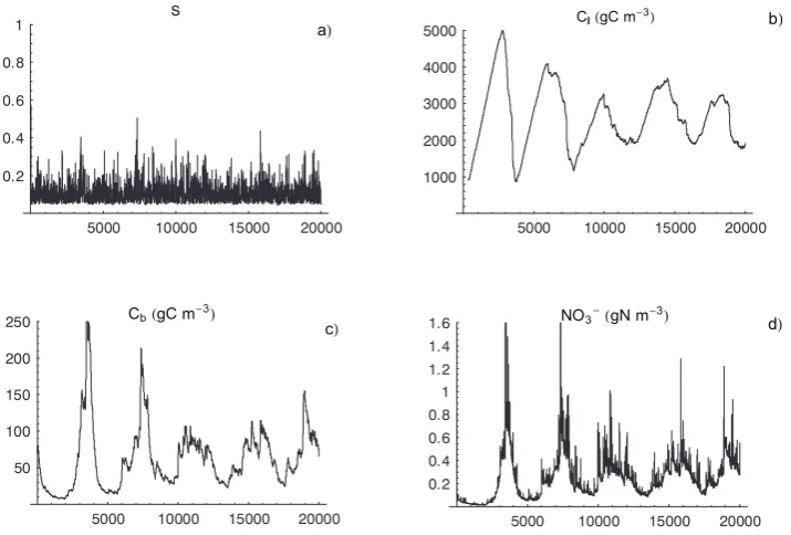
These results help explain the example of D’Odorico et al. (2003) under stochastic hydrologic conditions, where the system approached statistically steady conditions through damped oscillations having time scales of several growing seasons and amplitudes considerably larger than those in-duced by the stochastic hydrologic forcing (see Fig. 7). Such a behavior suggests that the soil nutrient system might show cases of richer (maybe chaotic) dynamics especially when the coupling with vegetation dynamics is considered. 4.2 Immobilization and basins of attraction
Fig. 6. Qualitative representation of the temporal dynamics of biomass (plots in the left column) and the biomass-carbon litter trajectories
(plots in the right column) for different soil moisture values.
temperature condition as well as for any value of(C/N)add
(which defines the total N entering the system). On the con-trary, initial conditions far from the steady state can cause oscillations of the dynamics leading to a sign change in net mineralization. After the mineralization has been halted, im-mobilization depletes the mineral nitrogen pool, until N be-comes limiting (ϕ < 1). Since the climatic conditions and the external input of added litter are kept (unrealistically) constant, there is no external variable able to force the system back to mineralization and the system comes to a complete stop (ϕ = 0). In reality, plant dynamics and hydroclimatic fluctuations, along with possible adaptations of the microbial community, are expected to contribute to avoid this hypothet-ical scenario.
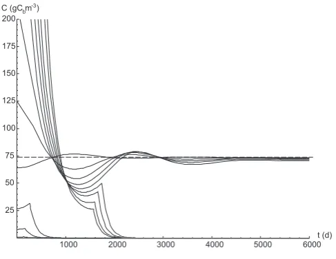
Figure 8 shows the temporal evolution of the biomass dy-namics, as a function of the initial condition (Cb,0=Cb(t=
0)). Soil moisture is kept constant, so that the only changing parameter isCb,0. It can be seen that for both very low and
very high initial values of biomass the system is attracted by the degenerate solution and does not approach the ’normal’ steady state solution. For low initial biomass, the system is not able to recycle enough dead biomass (BD) to enrich the litter pool with nitrogen: as a consequence, the living biomass tries to compensate the deficit of nutrients by im-mobilizing inorganic nitrogen. Net immobilization, however, can not be sustained by the system for a long period, because a net flux of mineral nitrogen from the soil to the biomass quickly depletes the mineralized nitrogen pool. As a conse-quence, the biomass begins to starve and its concentration in the soil decreases to zero. Similarly, when the initial biomass is very high, its request of nitrogen can not be met by SOM or mineral nitrogen, resulting in a system locking. Only in-termediate values, in the range 30–600 gC m−3, lead to sta-ble solutions through damped oscillations whose amplitude increases with the difference betweenCb,0andCb,eq.
From the dynamical system viewpoint, this means that, globally, the model presents two different asymptotic solu-tions: a steady state solution, determined analytically from the full system (Eqs. 1–7), and a degenerate one, correspond-ing toϕ =0. The latter is only partially stable, since some state variables continue to increase (in fact, forϕ → 0,Cl,
Nl, andCh in Eqs. 15–17 tend to infinity). Such solutions
correspond to two different basins of attraction, depending on both the climatic conditions and the initial conditions of the state variables.
5 Conclusions
Using a simple model of soil biogeochemistry, we have an-alyzed the possibility that nonlinear interactions and feed-backs among the variables may cause qualitative changes in the system response to environmental forcing, such as the presence of internal oscillations for some soil moisture and temperature conditions and sharp nonlinear transitions in the dynamics of the MIT turnover.
Fig. 8. Temporal dynamics of carbon in the biomass pool (Cb) for different initial conditions,Cb,0 = Cb(t = 0). In all cases,s = 0.15;(C/N)add = 140; the dashed line represents the steady state
solution.
Despite the idealized vegetation and climate conditions and the several simplifying hypotheses used in the analy-sis, the theoretical results derived here highlight the effects of internal nonlinearities and help to bring out the origin of the strong sensitivity to external fluctuations of soil biogeo-chemical cycles. A relaxation of such hypotheses as well as a more detailed representation of biogeochemical processes, and especially of their nonlinearities (both internal and in the response to external perturbations), is expected to result in even more complex system responses. Preliminary results were reported by D’Odorico et al. (2003) who investigated the dynamics of biogeochemical cycles under stochastic rain-fall forcing. Along different lines, the inclusion of a more re-alistic control of the microbial C/N ratio on the MIT turnover (e.g. by widening the range of C/N ratio of the decomposing community or by allowing some form of adaptation to nitro-gen poor conditions) and the inclusion of temporal variability in litter input and plant uptake would cure some pathological effects that the present model has pointed out when a strict C/N control of MIT is employed. A similar analytical inves-tigation of the implications of new paradigms in the soil car-bon and nitrogen cycles – regarding the role of plant uptake of organic nitrogen as well as the leaching of dissolved or-ganic nitrogen (Neff et al., 2003; Schimel and Bennett, 2004) – would be equally interesting.
Acknowledgements. We thank A. Guswa and an anonymous
reviewer for their useful comments. This research has been supported by the DOE-NIGEC (Great Plains Regional Center) grant DE-FC02-03ER63613 and the NSF grant EAR-0236621 (Hydrologic Sciences).
Edited by: B. Sivakumar
Reviewed by: A. Guswa and another referee
References
Argyris, J., Faust, G., and Haase, M.: An Exploration of Chaos, North Holland, 1994.
Baisden, W. T., Amundson, R.: An analytical approach to ecosys-tem biogeochemistry modeling, Ecol. Appl., 13, 3, 649–663, 2003.
Benbi, D. K. and Richter, J.: A critical review of some approaches to modelling nitrogen mineralization, Bio. Fertil. Soils, 35, 168– 183, 2002.
Birkinshaw, S. J. and Ewen, J.: Nitrogen transformation component for SHETRAN catchment nitrate transport modelling, J. Hydrol., 230, 1–17, 2000.
Bolker, B. J., Pakala, S. W., and Pakala, W. J.: Linear analysis of soil decomposition: insights from the century model, Ecol. Appl., 8, 2, 425–439, 1998.
Brady, N. C. and Weil, R. R.: The Nature and Properties of Soil, 11thed. Upper Saddle River, New Jersey, Prentice Hall, 1996. Cabon, F., Girard, G., and Ledoux, E.: Modelling of the nitrogen
cycle in farm land areas, Fertilizer Res., 27, 161–169, 1991. Cui, M. and Caldwell, M. M.: A large ephemeral release of nitrogen
upon wetting soil and corresponding root responses in the field, Plant and Soil, 191, 291–299, 1997.
D’Odorico, P., Laio, F., Porporato, A., and Rodriguez-Iturbe, I.: Hydrologic control on soil carbon and nitrogen cycles II a case study, Adv. Water Res., 26, 59–70, 2003.
Fierer, N. and Schimel J. P.: Effects of drying-rewetting frequency on soil carbon and nitrogen transformations, Soil Biol. Biochem., 34, 6, 777–787, 2002.
Freckman, D. W.: The ecology of dehydration in soil organisms, edited by Leopold, A. C., Membranes, Metabolism and Dry Or-ganisms, Ithaca, Cornell University Press, 157–168, 1986. Gusman, A. J. and Marino, M. A.: Analytical modeling of nitrogen
dynamics in soils and ground water, J. Irrig. Drainage Eng., 125, 6, 330–337, 1999.
Hansen, S., Jensen, H. E., and Shaffer , M. J.: Developments in modeling nitrogen transformation in soils, Nitrogen Fertilization in the Environment, edited by Bacon, P. E., Marcel Dekker Inc., New York, 1995.
Hunt, H. W., Trlica, M. J., Redente, E. F., Moore, J. C., Detling, J. K., Kittel, T. G. F., Walter, D. E., Fowler, M. C., Klein, D. A., and Elliott E. T.: Simulation model for the effects of climate change on temperate grasslands ecosystems, Ecol. Modell., 53, 205–246, 1991.
Jansson, S. L. and Persson, J.: Mineralization and immobilization of soil nitrogen, in Stevenson, F. J. (Ed.), Nitrogen in Agricultural Soils, Agron., 22, Am. Soc. Agron., Crop Sci. Soc. Am., Soil Sci. Soc. Am., Madison, WI, 229-252, 1982.
Katterer, T. and Andr`en, O.: The ICBM family of analytically solved models of soil carbon, nitrogen and microbial biomass dynamics – description and application examples, Ecol. Modell., 136, 191–207, 2001.
Kaye, J. P. and Hart, S. C.: Competition for nitrogen between plants and soil microorganisms, Trends Ecol. Evol., 12, 139–143, 1997. Laio, F., Porporato, A., Ridolfi, L., and Rodriguez-Iturbe, I.: Plants in water-controlled ecosystems. Active role in hydrological pro-cesses and response to water stress, II Probabilistic soil moisture dynamics, Adv. Water Res., 24, 7, 707–723, 2001.
Mary B., Recous S., Darwis D., and Robin D.: Interactions be-tween decomposition of plant residues and nitrogen cycling in soil, Plant and Soil, 181, 71–82, 1996.
Melillo J. M., Borchers J., and Chaney J.: Vegetation ecosystem modeling and analysis project – Comparing biogeography and biogeochemistry models in a continental-scale study of terres-trial ecosystem responses to climate change and CO2doubling,
Global Biogeochem. Cycles, 9, 4, 407–437, 1995.
Molina J. A. and Smith P.: Modeling carbon and nitrogen processes in soils, Adv. Agron., 62, 253–298, 1998.
Mueller, T., Magid, J., Jensen, L. S., Svendsen, H., and Nielsen, N. E.: Soil C and N turnover after incorporation of chopped maize, barley straw and blue grass in the field: evaluation of the DAISY soil-organic-matter submodel, Ecol. Modell., 111, 1–15, 1998.
Neff, J. C., Chapin, F. S., anc Vitousek, P. M.: Breaks in the cycle: dissolved organic nitrogen in terrestrial ecosystems, Frontiers in Ecology and the Environment, 1, 4, 205–211, 2003.
Parton, W. J., Stewart, J. W. B., and Cole, C. V.: Dynamics of C, N, P and S in grasslands soil: a model, Biogeochemistry, 5, 109– 131, 1988.
Porporato, A., Laio, F., Ridolfi, L., and Rodriguez-Iturbe, I.: Plants in water-controlled ecosystems, Active role in hydrological pro-cesses and response to water stress. III Vegetation water stress, Adv. Water Res., 24, 7, 725–744, 2001.
Porporato, A., D’Odorico, P., Laio, F., and Rodriguez-Iturbe, I.: Hydrologic controls on Soil carbon and nitrogen cycle I: Mod-elling scheme, Adv. Water Res., 26, 45–58, 2003.
Ratkowsky, D. A., Olley, J., McMeekin, T. A., and Ball, A.: Re-lationship between temperature and growth rate of bacterial cul-tures, J. Bacteriol., 149, 1, 1–5, 1982.
Schimel J. P. and Weintraub M. N.: The implications of exoenzyme activity on microbial carbon and nitrogen limitation in soil: a theoretical model, Soil Biol. Biochem., 35, 4, 549–563, 2003. Schimel J. P. and Bennett J.: Nitrogen mineralization: challenges of
a changing paradigm, Ecology, 85, 3, 591–602, 2004.
Scholes, R. J. and Walker B. H.: An African savanna, Cambridge University Press, 1993.
Vitousek P. M. and Howarth R. W.: Nitrogen limitation on land and in the sea – How can it occur, Biogeochemistry, 13, 2, 87–115, 1991 .