www.climate-of-the-past.net/cp/1/1/ SRef-ID: 1814-9332/cp/2005-1-1 European Geosciences Union
Climate
of the Past
Quantifying the effect of vegetation dynamics on the climate of the
Last Glacial Maximum
A. Jahn1,2, M. Claussen1,3, A. Ganopolski1, and V. Brovkin1
1Potsdam Institute for Climate Impact Research (PIK), P.O. Box 601203, 14412 Potsdam, Germany
2Now at Department of Atmospheric and Oceanic Sciences, McGill University, Burnside Hall Room 945, 805 Sherbrooke Street West, Montreal, Quebec, H3A 2K6, Canada
3Institute of Physics, Potsdam University, P.O. Box 601543, 14415 Potsdam, Germany Received: 13 June 2005 – Published in Climate of the Past Discussions: 23 June 2005 Revised: 19 September 2005 – Accepted: 22 September 2005 – Published: 4 October 2005
Abstract. The importance of the biogeophysical atmosphere-vegetation feedback in comparison with the radiative effect of lower atmospheric CO2concentrations and the presence of ice sheets at the last glacial maximum (LGM) is investigated with the climate system model CLIMBER-2. Equilibrium experiments reveal that most of the global cooling at the LGM (−5.1◦C) relative to (natural) present-day conditions is caused by the introduction of ice sheets into the model (−3.0◦C), followed by the effect of lower atmospheric CO2 levels at the LGM (−1.5◦C), while a synergy between these two factors appears to be very small on global average. The biogeophysical effects of changes in vegetation cover are found to cool the global LGM climate by 0.6◦C. The latter are most pronounced in the northern high latitudes, where the taiga-tundra feedback causes annually averaged temperature changes of up to −2.0◦C, while the radiative effect of lower atmospheric CO2 in this region only produces a cooling of 1.5◦C. Hence, in
this region, the temperature changes caused by vegetation dynamics at the LGM exceed the cooling due to lower atmospheric CO2concentrations.
1 Introduction
The climate at the Last Glacial Maximum (LGM) around 21 kyr BP has already been modeled extensively in the past (e.g. PMIP, 2000). In most of these studies, the vegeta-tion distribuvegeta-tion was prescribed, either to proxy-based re-constructions or to the present-day potential vegetation dis-tribution. In contrast to the potential present-day vegeta-tion cover, vegetavegeta-tion reconstrucvegeta-tions for the LGM show that forests were absent north of 55◦N, allowing herbaceous
veg-Correspondence to: A. Jahn
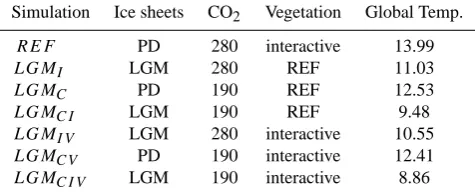
Table 1. Setup for all simulations. “PD” stands for present-day ice sheet forcing, “LGM” for LGM ice sheet forcing according to Peltier (1994). “280” and “190” stand for pre-industrial (i.e. “nat-ural” present-day) and LGM atmospheric CO2levels, respectively. “REF” stands for the use of a prescribed potential present-day veg-etation distribution as simulated inREFwhile “interactive” stands for the use of the interactive vegetation model. The last column shows the simulated globally averaged annual mean surface air tem-perature of each simulation (in◦C).
Simulation Ice sheets CO2 Vegetation Global Temp.
REF PD 280 interactive 13.99 LGMI LGM 280 REF 11.03
LGMC PD 190 REF 12.53
LGMCI LGM 190 REF 9.48
LGMI V LGM 280 interactive 10.55
LGMCV PD 190 interactive 12.41
LGMCI V LGM 190 interactive 8.86
included only the biogeophysical vegetation feedback while Brovkin et al. (2002b) analyzed the effect of an interactive vegetation on the carbon cycle during the LGM with the same model.
Since the LGM climate has been simulated before with CLIMBER-2 (Ganopolski et al., 1998; Ganopolski, 2003), the goal of this study is to investigate the role of dynamic vegetation in comparison with the roles played by prescribed changes in ice-sheet cover and the radiative effect of a lower atmospheric CO2concentration in the simulation of the LGM in a consistent way. We analyze the influence of these pre-scribed changes in comparison with the biogeophysical veg-etation feedback to determine their individual contribution to the cooling at the LGM; however, we do not account for bio-geochemical effects. In difference to Ganopolski (2003), we use factor separation and feedback analysis instead of fac-tor analysis to investigate the climatic change caused by the different contributions. Due to this difference in technique, we can separate the pure contributions of CO2 change, ice sheet change and vegetation changes from synergistic effects between them. Furthermore, we are able to investigate the individual response of vegetation to lowered CO2 and im-posed ice sheets with feedback analysis. Hence, this study is complementary to the work of Ganopolski (2003).
After comparing the individual effects of ice sheet and CO2 changes on the global annual surface air temperature with vegetation feedbacks, the ice sheet and CO2factors are then compared with the results of Berger et al. (1996), who performed experiments with a 1-D radiative convective cli-mate model in order to separate astronomical-albedo effects from the effect of CO2changes. The comparison of vegeta-tion feedbacks with ocean feedbacks will be the subject of a complementary study.
2 Methods
2.1 Model
CLIMBER-2 is a coarse resolution climate system model of intermediate complexity. It has a resolution of 10◦in
lati-tude and 51◦in longitude. The atmospheric module is a 2.5 dimensional statistical-dynamical model and the ocean mod-ule is a multi-basin, zonally averaged ocean model with 20 uneven vertical levels that also includes a sea-ice model. The terrestrial vegetation model VECODE within CLIMBER-2 is a reduced-form dynamic global vegetation model (see Cramer et al., 2001), which simulates the dynamics of two plant functional types (PFTs), trees and grass, in response to changes in climate. The PFT fractions are parameterized as a continuous function of growing degree days (sum of mean daily temperature for days with a temperature above a cer-tain threshold, here 0◦C) and annual precipitation. A more detailed description of CLIMBER-2 and its performance can be found in Petoukhov et al. (2000), Ganopolski et al. (2001), and Brovkin et al. (2002a).
2.2 Experiments and LGM boundary conditions
Several equilibrium experiments were performed for this study, using either present-day or LGM configurations for ice sheet cover and atmospheric CO2concentration as well as interactive or fixed vegetation (see Table 1 for the setup of all simulations and Sect. 2.3 for a detailed explanation of these experiment). All experiments were integrated for 5000 years and the model output averaged over the last 10 years of the equilibrium state was analyzed in this paper.
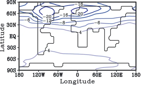
Fig. 1. Annually averaged surface air temperature differences (in ◦C) between the full LGM simulation (LGM
CI V) and the present-day reference runREF.
2.3 Factor separation and feedback analysis
To quantify the individual contributions of the prescribed changes in CO2 concentration and ice sheet cover, a factor separation was performed following Stein and Alpert (1993). They developed this technique to separate pure contribu-tions of different processes in a climate change signal from synergistic effects that result from non-linear processes in the climate system (Berger, 2001). In order to separate the pure contribution ofn factors from the synergies between them, 2n simulations are necessary. Therefore four simula-tions were necessary: a present-day reference run (REF); a simulation with LGM ice sheets but reference CO2 con-centration (LGMI); a simulation with LGM CO2 concentra-tion but reference ice cover (LGMC); and a run with both LGM ice sheets and LGM CO2 concentration (LGMCI). From the surface air temperatures at the end of these sim-ulations (T0,TI,TC,TCI, respectively), the two factors and the synergy term (caused by simultaneous changes in CO2 concentration and ice sheet cover) were calculated following Stein and Alpert (1993), i.e.fI=TI−T0,fC=TC−T0, and fCI=TCI−(TC−T0)−(TI−T0)−T0.
To compare the temperature changes due to the changes in CO2 concentration and ice sheet cover with the tem-perature change caused by the vegetation feedbacks in response to the cooling caused by CO2 and ice sheet changes, a feedback analysis was performed. For this feedback analysis, three more experiments were neces-sary: a simulation with LGM CO2 concentration and interactive vegetation (LGMCV); a run with LGM ice sheets and interactive vegetation (LGMI V); and a sim-ulation with LGM ice sheets, LGM CO2, and interac-tive vegetation (LGMCI V). These simulations provided the surface air temperaturesTCV, TI V, andTCI V, respec-tively. The feedback factors fIV, fCV, and fCIV were then calculated as follows: fCV=TCV−TC, fIV=TI V−TI, and fCIV =TCI V−TCI−(TCV−TC)−(TI V−TI).
Table 2. Annual averaged global temperature changes caused by the ice sheet factor (fI), the CO2factor (fC), their synergy term (fCI), the vegetation feedback to the climatic change caused by the ice sheet factor (fIV), the vegetation feedback to the climatic change caused by the CO2factor (fCV), and the vegetation feedback to the climatic change caused by the synergy term (fCIV ). The calculation of these terms is described in Sect. 2.3.
Factors Change in◦C Feedbacks Change in◦C
fI −2.96 fIV −0.48
fC −1.46 fCV −0.12
fCI −0.09 fCIV −0.02
In the factor separation, the forcing is prescribed, while in the feedback analysis, the feedback is a factor of the state of the system and it changes in response to the forcing. Here we have chosen ice sheets and CO2 as forcing/factor, be-cause ice sheets and CO2are not simulated interactively in the present version of CLIMBER. In both factor separation and feedback analysis, the same terms, such as pure contribu-tion and synergy, appear, but there are different assumpcontribu-tions behind them. In the factor separation, the termfCreflects the response of the system to CO2forcing. In the feedback anal-ysis, the termfCV reflect the response of the system to the vegetation changes that occur as reaction to the CO2 forc-ing. The synergy termfCI depicts the additional response of the system to applying both forcings, CO2and ice sheets, simultaneously. The synergy termfCIV shows the additional climate response due to the vegetation feedback to simulta-neously applied CO2and ice sheets forcing.
3 Results
The LGM climate simulated in the full LGM experiment (LGMCI V) shows a global annual mean surface air temper-ature of 8.9◦C, which is 5.1◦C lower than in the present-day
reference run (REF). This temperature decrease is in the range of simulated changes from AOGCMs that find a LGM cooling between 3.8◦C (Hewitt et al., 2003) and 10◦C (Kim et al., 2003). The cooling is centered over the ice sheets of the northern hemisphere (NH) and is much weaker over the southern hemisphere (SH) (Fig. 1).
This global LGM cooling of 5.1◦C can be attributed to
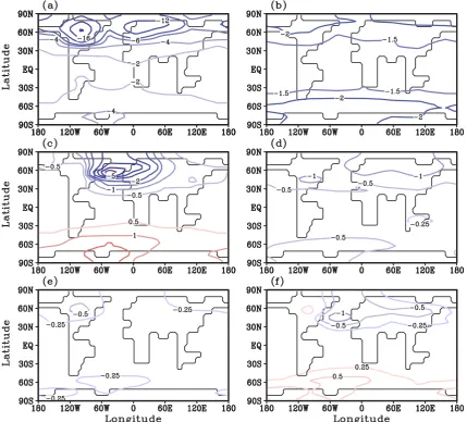
Fig. 2. Annually averaged surface air temperature changes (in◦C) caused by (a) the presence of an ice sheet (fI), (b) lowering of CO2to 190 ppm (fC), (c) synergy between ice sheets and CO2decrease (fCI), (d) vegetation change in response to an ice sheet (fIV), (e) vegetation change in response to the lowered CO2(fCV), and (f) vegetation change in response to the synergy between presence of ice sheets and CO2 lowering (fCIV ).
cooling produced by the LGM ice sheets, leads to an addi-tional global temperature decrease of 0.5◦C. The vegetation
feedback to the cooling caused by the lower CO2(fCV) pro-duces a cooling of 0.1◦C, which is the same amount of cool-ing as generated byfCI (the additional temperature change due to the simultaneous CO2 and ice sheet change). The vegetation feedback to the cooling caused by the synergy between CO2 and ice sheet forcing (fCIV ) leads to a global temperature decrease of substantially less than 0.1◦C.
As shown in Fig. 2, there is considerable variation in the regional distribution of the cooling due to each of these fac-tors/feedback terms. The presence of ice sheets causes a cooling mainly over the ice covered regions of the NH due to the increase in albedo and altitude (Fig. 2a). The cool-ing in the NH leads to an increase in the Atlantic overturncool-ing
Fig. 3. (a) Change in the annually averaged surface air temperature due to the biogeophysical vegetation feedbacks (in◦C) and (b) the associated change in fractional tree coverage compared to the prescribed potential present-day vegetation cover (i.e. vegetation change betweenLGMCI andLGMCI V). The blue line in (b) represents the boundary of 60% inland ice coverage within a grid cell.
in the SH, which explains the stronger cooling in the high latitudes of the SH compared to the NH. The synergy fac-torfCI produces a strong cooling over the North Atlantic and a warming over the Southern Ocean (Fig. 2c). This tem-perature change is caused by a decrease in northward heat transport in the ocean and a displacement of the deep wa-ter formation site to the south, which means that the ocean circulation changes from its “warm” mode (in which it is in REF,LGMI, andLGMC) to its “cold” mode (inLGMCI) (see Ganopolski and Rahmstorf, 2001, Fig. 2).
As shown in Ganopolski and Rahmstorf (2001), the bi-furcation transition between cold and warm modes occurs in the domain of negative anomalous freshwater forcing for the full glacial conditions. However, for a somewhat warmer cli-mate, the position of bifurcation transition moves to the do-main of positive freshwater flux, i.e. the warm mode becomes stable under zero freshwater anomalous flux. Thereby the global cooling is another bifurcation parameter of the model, and for unperturbed freshwater flux, the global temperature determines which mode of the thermohaline circulation is stable. The critical temperature threshold is crossed in this study when CO2and ice sheets are changed simultaneously to LGM conditions (i.e. inLGMCI). As intended by Stein and Alpert (1993), the effect of this non-linear climate re-sponse is captured by the synergy termfCI. However, sen-sitivity studies show that the combined cooling due to CO2 decrease and presence of ice sheets is just large enough to trigger the change in the ocean circulation. A slightly smaller cooling, as caused for example by a CO2 concentration of 200 ppm instead of 190 ppm in combination with ice sheets, does not cause this change in the ocean circulation mode. In this case, the additional cooling produced by the vegeta-tion feedback triggers the change in the ocean circulavegeta-tion, and the large temperature change associated with it is then included in the termfCIV . This could lead to a misinterpre-tation of the termfCIV , since the large temperature change is not produced by vegetation feedbacks per se, but by a nonlin-ear process that is only triggered by the effect of vegetation
feedbacks. Therefore, care has to be taken to not confuse the effect of non-linear processes with the effect of climate feed-backs when calculating individual contributions of feedfeed-backs close to bifurcation points in the climate system.
The cooling effect of fIV is strongest over land in the northern high latitudes (Fig. 2d). It is due to the replacement of forest by herbaceous vegetation in response to the cool-ing caused by the ice sheet factor (fI), which increases the albedo of these regions especially in winter and spring when the surface is snow covered (see Brovkin et al., 2003). In ad-dition, this so called taiga-tundra feedback is amplified by an increase in snow coverage over these regions. The cooling generated byfCV is strongest over North America (Fig. 2e), as a result of the taiga-tundra feedback in this region. As seen in Fig. 2f,fCIV causes the strongest cooling over the North Atlantic and northern latitudes of Eurasia, combined with a warming of the Southern Ocean. The cooling over the North Atlantic is a result of a further decrease of the northward heat transport and an associated increase in sea-ice cover com-pared toLGMCI. The decrease in northward heat transport is also responsible for the warming in the SH. In the northern latitudes of Eurasia,fCIV shows a cooling over regions where tree cover decreases, again due to the taiga-tundra feedback. To compare the cooling caused by the total vegetation feedback with the radiative effect of lowered atmospheric CO2 concentrations, the temperature changes of all three vegetation feedback terms are added (Fig. 3a). Over the land areas of northern Siberia, the combined effect of the vegeta-tion changes leads to a cooling of about 2◦C, while the CO2 reduction to 190 ppm infC (Fig. 2b) causes a temperature decrease of 1.5◦C in this region. This strong cooling by the
To evaluate the results of this study, the temperature changes caused by the factorsfI andfCare compared with the factors calculated by Berger et al. (1996). They found that the increase in albedo due to the presence of an LGM ice sheet, combined with the changed orbital parameters, leads to a cooling of 3.0◦C at the LGM, while the lowering of the CO2level by 136 ppm cooled the climate by 1.6◦C. In CLIMBER-2, the presence of an ice sheet causes a temper-ature change of−3.0◦C, and even if we add the very small effect of changed orbital parameters and its synergy with ice sheets (as found in sensitivity studies), the cooling by the ice sheet and orbital parameter factor still is 3.0◦C. The lower-ing of the CO2level by 90 ppm to 190 ppm produces a cool-ing of 1.5◦C in CLIMBER-2. Together with the small posi-tive synergy factor between these two factors, Berger et al. (1996) found a LGM cooling of 4.5◦C. This is the same
cooling as found in the CLIMBER-2 simulation with fixed present-day vegetation (i.e. experimentLGMCI). The larger CO2 decrease of 136 ppm in Berger et al. (1996) caused a temperature change for the CO2 factor that is only slightly larger than the one found in CLIMBER-2 with a CO2 reduc-tion of only 90 ppm. This is consistent with the smaller sen-sitivity of the model of Berger et al. (1996) to a doubling of CO2 (1.8◦C), as compared with the CO2 sensitivity of CLIMBER-2 (2.6◦C). Therefore, it can be concluded that the individual effects of the factorsfI andfCare consistent with the results of Berger et al. (1996).
4 Conclusions
Although globally the biogeophysical effect of vegetation dynamics on air temperature is less important for the LGM climate than the impact of CO2changes and the presence of ice sheets, it was shown that in the northern high latitudes of Eurasia vegetation changes have a cooling effect that exceeds the temperature decrease due to the CO2decrease in this re-gion. Hence, the use of a dynamic vegetation module instead of a prescribed present-day vegetation distribution is impor-tant as it causes significant temperature changes on a re-gional scale. This is especially important for the LGM, since Brovkin et al. (2003) showed that climate-vegetation inter-actions in the northern high latitudes are stronger in colder climates than in warmer climates, due to a longer snow sea-son in colder climates that increases the radiative effect of the taiga-tundra effect in northern latitudes.
Furthermore, the factor separation showed that in CLIMBER-2 the influence of the CO2 drop at the LGM is distributed over both hemispheres; however, it is stronger over the SH due to ocean effects. The cooling caused by the ice sheets is strongest over the ice covered regions of the NH. A comparison of the globally averaged cooling caused by the presence of ice sheets and CO2reduction at the LGM with the results of Berger et al. (1996) shows that these two factors are in good agreement in both studies.
Acknowledgement. The authors would like to thank C. Kubatzki for constructive discussions and M.-F. Loutre, S. Levis, L. A. Mysak and an anonymous referee for helpful comments that improved the manuscript. During the preparation of the actual manuscript, A. Jahn was supported by a Canadian NSERC Discovery Grant awarded to L. A. Mysak.
Edited by: G. M. Ganssen
References
Berger, A.: The role of CO2, sea-level and vegetation during the Milankovitch-forced glacial-interglacial cycles, in: Geosphere-Biosphere Interactions and Climate, Proceedings of the work-shop held at Pontifical Academy of Science, edited by: Bengts-son, L. O. and Hammer, C. U., Cambridge University Press, 119– 146, 2001.
Berger, A., Dutrieux, A., Loutre, M. F., and Tricot, C.: Paleoclimate sensitivity to CO2and insolation, Scientific Report 1996/6, Insti-tut d’Astronomie et G´eophysique Georges Lemaˆıtre, Universit´e Catholique de Louvain, Louvain-la-Neuve, 1996.
Bigelow, N. H., Brubaker, L. B., Edwards, M. E., Harrison, S. P., Prentice, I. C., Anderson, P. M., Andreev, A. A., Bartlein, P. J., Christensen, T. R., Cramer, W., Kaplan, J. O., Lozhkin, A. V., Matveyeva, N. V., Murray, D. F., McGuire, A. D., Gajewski, K., Wolf, V., Holmqvist, B. H., Igarashi, Y., Kremenetskii, K., Paus, A., Pisaric, M. F. J., and Volkova, V. S.: Climate change and Arctic ecosystems: 1. Vegetation changes north of 55◦N be-tween the last glacial maximum, mid-Holocene, and present, J. Geophys. Res., 108, doi: 10.1029/2002JD002 558, 2003. Brovkin, V., Claussen, M., Ganopolski, A., Bendtsen, J.,
Ku-batzki, C., Petoukhov, V., and Andreev, A.: Carbon Cycle, veg-etation and climate dynamics in the Holocene: Experiments with the CLIMBER-2 model, Global Geochemical Cycles, 16, doi:10.1029/2001GB001 662, 2002a.
Brovkin, V., Hoffmann, M., Bendtsen, J., and Ganopolski, A.: Ocean biology could control atmospheric δ13C during glacial-interglacial cycle, Geochem., Geophys., Geosyst., 3, doi:10.1029/2001GC000 270, 2002b.
Brovkin, V., Levis, S., Loutre, M.-F., Crucifix, M., Claussen, M., Ganopolski, A., and C. Kubatzki, V. P.: Stability analysis of the climate-vegetation system in the northern high latitudes, Clim. Change, 57, 119–138, 2003.
Cramer, W., Bondeau, A., Woodward, F. I., Prentice, I. C., Betts, R. A., Brovkin, V., Cox, P. M., Fisher, V., Foley, J., Friend, A. D., Kucharik, C., Lomas, M. R., Ramankutty, N., Sitch, S., Smith, B., White, A., and Young-Molling, C.: Dynamic responses of global terrestrial ecosystems to changes in CO2 and climate, Global Change Biol., 7, 357–373, 2001.
Crowley, T. J. and Baum, S.: Effect of vegetation on an ice-age climate model simulation, J. Geophys. Res., 102, 463–480, 1997. Ganopolski, A.: Glacial integrative modelling, Phil. Trans. Royal.
Soc. Lond., 361, 1871–1884, 2003.
Ganopolski, A. and Rahmstorf, S.: Rapid changes of glacial cli-mate simulated in a coupled clicli-mate model, Nature, 409, 153– 158, 2001.
Ganopolski, A., Petoukhov, V., Rahmstorf, S., Brovkin, V., Claussen, M., Eliseev, A., and Kubatzki, C.: CLIMBER-2: a climate system model of intermediate complexity, Part II: model sensitivity, Clim. Dyn., 17, 735–751, 2001.
Harrison, S. P. and Prentice, C. I.: Climate and CO2 controls on global vegetation distribution at the last glacial maximum: analy-sis based on palaeovegetation data, biome modelling and palaeo-climate simulations, Global Change Biol., 9, 983–1004, 2003. Hewitt, C. D., Stouffer, R. J., Broccoli, A. J., Mitchell, J. F. B., and
Valdes, P. J.: The effect of ocean dynamics in a coupled GCM simulation of the Last Glacial Maximum, Clim. Dyn., 20, 203– 218, 2003.
Kim, S.-J., Flato, G. M., and Boer, G. J.: A coupled climate model simulation of the Last Glacial Maximum, Part 2: approach to equilibrium, Clim. Dyn., 20, 635–661, 2003.
Kubatzki, C. and Claussen, M.: Simulation of the global bio-geophysical interactions during the Last Glacial Maximum, Clim. Dyn., 14, 461–471, 1998.
Levis, S., Foley, J. A., and Pollard, D.: CO2, climate, and vegetation feedbacks at the Last Glacial Maximum, J. Geophys. Res., 104, 191–198, 1999.
Peltier, W. R.: Ice Age Paleotopography, Science, 256, 195–201, 1994.
Petit, J. R., Jouzel, J., Raynaud, D., Barkov, N. I., Barnola, J.-M., Basile, I., Bender, M., Chappellaz, J., Davis, M., Delaygue, G., Delmotte, M., Kotlyakov, V. M., Legrand, M., Lipenkov, V. Y., Lorius, C., Pepin, L., Ritz, C., Saltzman, E., and Stievenard, M.: Climate and atmospheric history of the past 420,000 years from the Vostok ice core, Antarctica, Nature, 399, 429–436, 1999. Petoukhov, V., Ganopolski, A., Brovkin, V., Claussen, M., Eliseev,
A., Kubatzki, C., and Rahmstorf, S.: CLIMBER-2: a climate system model of intermediate complexity, Part I: model descrip-tion and performance for present climate, Clim. Dyn., 16, 1–17, 2000.
PMIP: Paleoclimate Modeling Intercomparison Project (PMIP), in: Proceedings of the third PMIP workshop, edited by Braconnot, P., vol. WCRP-111, WMO/TD-1007, p. 271, Canada, 2000. Stein, U. and Alpert, P.: Factor Separation in numerical simulations,
J. Atmos. Sci., 50, 2107–2115, 1993.