www.the-cryosphere.net/9/1721/2015/ doi:10.5194/tc-9-1721-2015
© Author(s) 2015. CC Attribution 3.0 License.
Exploring the utility of quantitative network design in evaluating
Arctic sea ice thickness sampling strategies
T. Kaminski1,a, F. Kauker2, H. Eicken3, and M. Karcher2 1The Inversion Lab, Martinistr. 21, 20251 Hamburg, Germany 2OASys, Lerchenstraße 28a, 22767 Hamburg, Germany
3Geophysical Institute and International Arctic Research Center, University of Alaska Fairbanks, P.O. Box 757320, Fairbanks, AK 99775-7320, USA
aformerly at: FastOpt, Hamburg, Germany
Correspondence to: T. Kaminski ([email protected])
Received: 3 March 2015 – Published in The Cryosphere Discuss.: 19 March 2015 Revised: 24 July 2015 – Accepted: 9 August 2015 – Published: 27 August 2015
Abstract. We present a quantitative network design (QND) study of the Arctic sea ice–ocean system using a software tool that can evaluate hypothetical observational networks in a variational data assimilation system. For a demonstra-tion, we evaluate two idealised flight transects derived from NASA’s Operation IceBridge airborne ice surveys in terms of their potential to improve 10-day to 5-month sea ice forecasts. As target regions for the forecasts we select the Chukchi Sea, an area particularly relevant for maritime traf-fic and offshore resource exploration, as well as two areas related to the Barnett ice severity index (BSI), a standard measure of shipping conditions along the Alaskan coast that is routinely issued by ice services. Our analysis quantifies the benefits of sampling upstream of the target area and of reducing the sampling uncertainty. We demonstrate how ob-servations of sea ice and snow thickness can constrain ice and snow variables in a target region and quantify the com-plementarity of combining two flight transects. We further quantify the benefit of improved atmospheric forecasts and a well-calibrated model.
1 Introduction
The Arctic climate system is undergoing a rapid transforma-tion. Such changes, in particular reductions in sea ice ex-tent, are impacting coastal communities and ecosystems and are enhancing the potential for resource extraction and ship-ping. In this context, the ability to anticipate anomalous ice
conditions and in particular sea ice hazards associated with seasonal-scale and short-term variations in ice cover is es-sential. For example, in 2012, despite a long-term trend of greatly reduced ice cover in the Chukchi Sea off Alaska’s coast, ice incursions and associated hazards led to early ter-mination of the resource exploration season (Eicken and Ma-honey, 2015). In this context, high-quality predictions of the ice conditions are of paramount interest. Such predictions are typically performed by numerical models of the sea ice– ocean system. These models are based on fundamental equa-tions that govern the processes controlling ice condiequa-tions. Uncertainty in model predictions arises from four sources: first, there is uncertainty in the atmospheric forcing data (such as wind velocity or temperature) driving the relevant processes. Second, there is uncertainty regarding the formu-lation of individual processes and their numerical implemen-tation (structural uncertainty). Third, there are uncertain con-stants (process parameters) in the formulation of these pro-cesses (parametric uncertainty). Fourth, there is uncertainty about the state of the system at the beginning of the simula-tion (initial state).
1722 T. Kaminski et al.: Evaluating Arctic sea ice thickness sampling strategies by the model to yield a consistent picture of the state of the
Arctic system that balances all the observational constraints, taking into account the respective uncertainty ranges. Data assimilation systems that tie into prognostic models of the Arctic system are ideal tools for this integration task because they allow a variety of observations to be combined with the simulated dynamics of a model.
Quantitative network design (QND) is a technique that aims to design an observational network with optimal per-formance. The approach is based on work by Hardt and Scherbaum (1994), who optimised the station locations for a seismographic network. It was first applied to the climate system by Rayner et al. (1996), who optimised the spatial distribution of atmospheric measurements of carbon diox-ide. A series of QND studies (Rayner and O’Brien, 2001; O’Brien and Rayner, 2002; Rayner et al., 2002) demon-strated the feasibility of the network design approach and de-lineated the requirements for the implementation of the first satellite mission designed to observe atmospheric CO2from space (the Orbiting Carbon Observatory; Crisp et al., 2004). Since then, the technique has been routinely applied in the design of CO2space missions (Patra et al., 2003; Kadygrov et al., 2009; Kaminski et al., 2010; Rayner et al., 2014) and the extension of the in situ sampling network for atmospheric carbon dioxide. Recent examples focus on in situ networks over Australia (Ziehn et al., 2014) and South Africa (Nick-less et al., 2014). The design of a combined atmospheric and terrestrial network of the European carbon cycle is addressed by Kaminski et al. (2012).
The present study applies the QND concept to the Arc-tic sea ice–ocean system. It describes the ArcArc-tic Observa-tional Network Design (AOND) system, a tool that can eval-uate the performance of observational networks comprising a range of different data streams. We illustrate the utility of the tool by evaluating the relative merits of alternate airborne transects within the context of NASA’s Operation IceBridge (Richter-Menge and Farrell, 2013; Kurtz et al., 2013a), as-sessing their potential to improve ice forecasts in the Chukchi Sea and along the Alaskan coast.
2 Methods
Our AOND system evaluates observational networks in terms of their impact on target quantities in a data assim-ilation system. Both the data assimassim-ilation system and the AOND system are built around the same model of the Arc-tic sea ice–ocean system. Below, we first present the model, then the assimilation system and finally the QND approach that operates on top of this model.
2.1 NAOSIM
The model used for the present analysis is the coupled sea ice–ocean model NAOSIM (North Atlantic/Arctic Ocean
Sea Ice Model; Kauker et al., 2003). NAOSIM is based on version 2 of the Modular Ocean Model (MOM-2) of the Geophysical Fluid Dynamics Laboratory. The version of NAOSIM used here has a horizontal grid spacing of 0.5◦on a rotated spherical grid. The rotation maps the 30◦W merid-ian onto the Equator and the North Pole onto 0◦E. Hence, the model’sx andy directions are different from the zonal and meridional directions, and the grid is almost equidistant. In the vertical it resolves 20 levels, their spacing increasing with depth from 20 to 480 m. At the southern boundary (near 50◦ N) an open boundary condition has been implemented fol-lowing Stevens (1991), alfol-lowing the outflow of tracers and the radiation of waves. The other boundaries are treated as closed walls. At the open boundary the barotropic transport is prescribed from a coarser-resolution version of the model that covers the whole Atlantic northward of 20◦S (Köberle and Gerdes, 2003).
A dynamic-thermodynamic sea ice model with a viscous-plastic rheology (Hibler, 1979) is coupled to the ocean model. The prognostic variables of the sea ice model are ice thickness, snow depth, and ice concentration. Ice drift is calculated diagnostically from the momentum balance. Snow depth and ice thickness are mean quantities over a grid box. The thermodynamic evolution of the ice is described by an energy balance of the ocean mixed layer following Parkin-son and Washington (1979). Freezing and melting are calcu-lated by solving the energy budget equation for a single ice layer with a snow layer. When atmospheric temperatures are below the freezing point, precipitation is added to the snow mass; otherwise it is added to the ocean. The snow layer is advected jointly with the ice layer. The surface heat flux is calculated through a standard bulk formula approach using prescribed atmospheric data and sea surface temperature pre-dicted by the ocean model. Owing to its low heat conductiv-ity, the snow layer has a high impact on the simulated energy balance (Castro-Morales et al., 2014). The sea ice model is formulated on the ocean model grid and uses the same time step. The models are coupled following the procedure de-vised by Hibler and Bryan (1987).
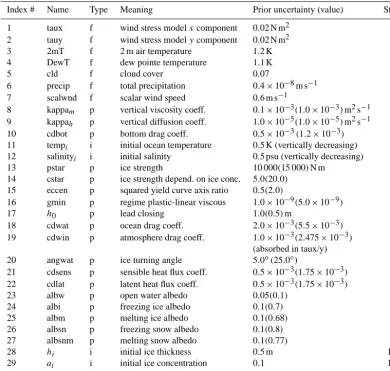
at-Table 1. Control variables. Column 1 lists the quantities in the control vector; column 2 gives the abbreviation for each quantity; column 3 indicates whether the quantity is an atmospheric boundary (forcing, i.e. f) field, an initial field (i), or a process parameter (p); column 4 gives the name of each quantity; column 5 indicates (the standard deviation of) the prior uncertainty and the corresponding units and provides the magnitude of the parameter value in parenthesis, where applicable; and column 6 identifies the position of the quantity in the control vector – for initial and boundary values (which are differentiated by region) this position refers to the first region, while the following components of the control vector then cover regions 2 to 9.
Index # Name Type Meaning Prior uncertainty (value) Start
1 taux f wind stress modelxcomponent 0.02 N m2 1
2 tauy f wind stress modelycomponent 0.02 N m2 10
3 2mT f 2 m air temperature 1.2 K 19
4 DewT f dew pointe temperature 1.1 K 28
5 cld f cloud cover 0.07 37
6 precip f total precipitation 0.4×10⁻⁸m s−1 46
7 scalwnd f scalar wind speed 0.6 m s−1 55
8 kappam p vertical viscosity coeff. 0.1×10⁻³(1.0×10⁻³)m2s−1 64
9 kappah p vertical diffusion coeff. 1.0×10⁻⁵(1.0×10⁻⁵)m2s−1 65
10 cdbot p bottom drag coeff. 0.5×10⁻³(1.2×10⁻³) 66
11 tempi i initial ocean temperature 0.5 K (vertically decreasing) 67
12 salinityi i initial salinity 0.5 psu (vertically decreasing) 76
13 pstar p ice strength 10 000(15 000)N m 85
14 cstar p ice strength depend. on ice conc. 5.0(20.0) 86
15 eccen p squared yield curve axis ratio 0.5(2.0) 87
16 gmin p regime plastic-linear viscous 1.0×10⁻⁹(5.0×10⁻⁹) 88
17 h0 p lead closing 1.0(0.5)m 89
18 cdwat p ocean drag coeff. 2.0×10⁻³(5.5×10⁻³) 90
19 cdwin p atmosphere drag coeff. 1.0×10⁻³(2.475×10⁻³)
(absorbed in taux/y)
20 angwat p ice turning angle 5.0◦(25.0◦) 92
21 cdsens p sensible heat flux coeff. 0.5×10⁻³(1.75×10⁻³) 93
22 cdlat p latent heat flux coeff. 0.5×10⁻³(1.75×10⁻³) 94
23 albw p open water albedo 0.05(0.1) 95
24 albi p freezing ice albedo 0.1(0.7) 96
25 albm p melting ice albedo 0.1(0.68) 97
26 albsn p freezing snow albedo 0.1(0.8) 98
27 albsnm p melting snow albedo 0.1(0.77) 99
28 hi i initial ice thickness 0.5 m 100
29 ai i initial ice concentration 0.1 109
30 hsni i initial snow thickness 0.2 m 118
mospheric forcing fields and initial fields, and lists a subset of the model’s relevant process parameters.
2.2 Assimilation
The variational assimilation system NAOSIMDAS (Kauker et al., 2009, 2010) operates through minimisation of a cost function that quantifies the fit to all observations plus the deviation from prior knowledge on a vector of control
vari-ablesx:
J (x)=1 2
h
(M(x)−d)TC(d)−1(M(x)−d)
+(x−x0)TC(x0)−1(x−x0)
i
, (1)
1724 T. Kaminski et al.: Evaluating Arctic sea ice thickness sampling strategies C(dmod)captures all uncertainty in the simulation of the
ob-servations except for the uncertainty in the control vector be-cause this fraction of the uncertainty is explicitly addressed by the assimilation procedure through correction of the con-trol vector.
The control vectorexthat minimises Eq. (1) achieves a bal-ance between the observational constraints and the prior in-formation. The minimum is determined through variation of the control vector (hence variational assimilation) compris-ing initial and boundary conditions and process parameters. In contrast to sequential assimilation approaches, which re-sult in a sequence of corrections of the state predicted by the model, the variational approach guarantees full consistency with the dynamics imposed by the model, as it provides an entire trajectory through the state space of the model in re-sponse to the change in the control vector. In the case of our model this means that we infer a trajectory that assures con-servation of mass, energy and momentum (except at the lat-eral domain boundaries). We note that, in this QND study, no minimisation of Eq. (1) is required.
2.3 QND
We provide a brief description of the methodological back-ground for QND, which follows Kaminski and Rayner (2008). The approach is based on propagation of uncertainty from the data to a target quantity of interest. The target quan-tity may be any aspect (e.g. a prognostic or diagnostic vari-able or a process parameter) that can be extracted from a sim-ulation with the underlying model, for example, the sea ice concentration integrated over a particular domain and time period.
QND proceeds in two steps. In the first step, the second derivative (Hessian) of the cost function (Eq. 1) is used to ap-proximate the inverse of the covariance matrix C(x)of pos-terior uncertainty of the control vector, which quantifies the uncertainty ranges of the control variables that are consistent with uncertainties in the observations and the model. Denot-ing the linearisation of the model by M0, we can approximate this posterior uncertainty by
C(x)−1=M0TC(d)−1M0+C(x0)−1. (3) The first term on the right-hand side quantifies the observa-tional impact which yields an uncertainty reduction with re-spect to the prior uncertainty (inverse of the second term).
When the prior uncertainty is already small, the second term is large, and a large observational impact is required to achieve a substantial uncertainty reduction. The observa-tional impact is large when the observations are highly sensi-tive to changes in the control variables and when the data un-certainty is small. The first condition describes the relevance of the observation, and the second condition its quality.
In the second step, the linearisation N0 (Jacobian) of the modelNused as a mapping from the control vector to target quantities is employed to propagate the uncertainties in the
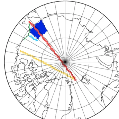
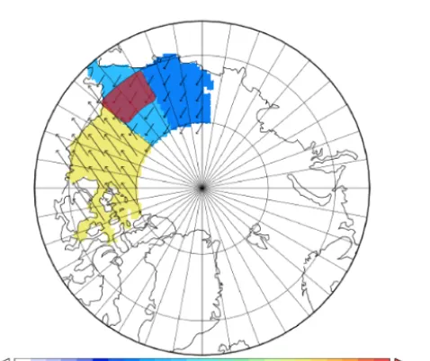
Figure 1. Target regions: Chukchi (dark blue); north of Barrow (NOB, light blue) Bering Strait to Prudhoe Bay (BS2PB, red). Flight transects: Chukchi to Fram (C2F, red); Beaufort to Fram (B2F, yellow).
control vector forward to the uncertainty in a target quantity
σ (y):
σ (y)2=N0C(x)N0T+σ (ymod)2. (4) If the model were perfect,σ (ymod) would be zero. In con-trast, if the control variables were perfectly known, the first term on the right-hand side would be zero. Equation (4) re-lates the uncertainty in control space to uncertainty in a target quantity.
Evaluating Eq. (4) for the prior uncertainty C(x0)instead of the posterior uncertainty C(x), i.e. for a case without ob-servational constraint, yields a prior uncertainty for the target quantity:
σ (y0)2=N0C(x0)N0T+σ (ymod)2. (5) We define the term uncertainty reduction relative toσ (y0), i.e. by
σ (y0)−σ (y)
σ (y0)
=1− σ (y)
σ (y0)
. (6)
For example, ifσ (y)is 90 % ofσ (y0), then the uncertainty reduction is 10%; i.e. we have increased our knowledge ony
by 10.
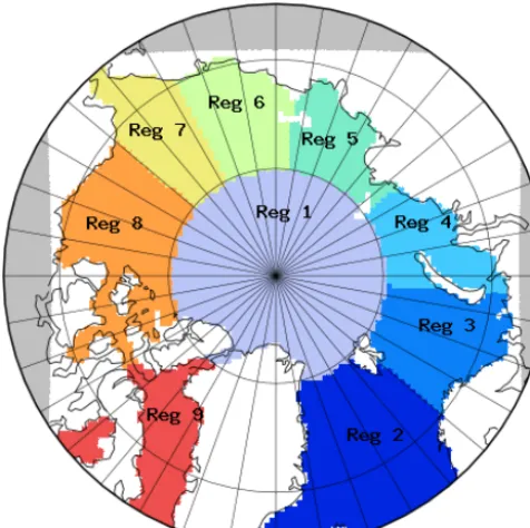
Figure 2. Sub-regions defined in the study. 1 (light plum): central Arctic. 2 (dark blue): North Atlantic; and then counterclockwise to 7 (yellow): Bering Strait/Chukchi Sea; 8 (orange): Beaufort Sea; 9 (red): Baffin Bay.
quantity. In other words, it does not help to constrain parts of the control space that have no impact on the target quantity (as quantified byN0). Specific examples and further discus-sion of how to interpret the matrix N0 will be provided in Sect. 4 below.
We note that (through Eqs. 3 and 4) the posterior target un-certainty solely depends on the prior and data uncertainties as well as the linearised model responses of simulated ob-servation counterparts and of target quantities. The approach does not require real observations and can thus be employed to evaluate hypothetical candidate networks. Candidate net-works are defined by a set of observations characterised by observational data type, location, time, and data uncertainty. Hence, the QND approach does not require running the as-similation system. Here, we define a network as the complete set of observations,d, used to constrain the model. The term network is not meant to imply that the observations are of the same type or that their sampling is coordinated. For example, a network can combine in situ and satellite observations.
In practice, for pre-defined target quantities and obser-vations, model responses can be pre-computed and stored. A network composed of these pre-defined observations can then be evaluated in terms of the pre-defined target quan-tities without further model evaluation. Only matrix alge-bra is required to combine the pre-computed sensitivities with the data uncertainties. This aspect is exploited in our AOND system. The linearised response functions were com-puted by the tangent linear version of NAOSIM generated
from the model’s source code through the automatic dif-ferentiation tool Transformation of Algorithms in Fortran (TAF; Giering and Kaminski, 1998).
3 Experimental setup 3.1 Target quantities
The goal of this study is to explore the utility of the AOND system in guiding observations for short-term to seasonal-scale sea ice predictions. Ice forecasting at these timeseasonal-scales has been identified as a high priority in the context of safe maritime operations (Richter-Menge and Walsh, 2012; Kurtz et al., 2013a; Eicken, 2013), management of marine living resources (Robards et al., 2013) and food security for indige-nous communities (Brubaker et al., 2011). Here, we focus on the first two issues in the Chukchi and Beaufort seas north of Alaska (Figs. 1 and 2), which are experiencing some of the highest reductions in summer ice concentration anywhere in the Arctic, along with major offshore hydrocarbon explo-ration and potential impacts on protected species such as wal-rus (Eicken and Mahoney, 2015). Thus, the selection of tar-get quantities for the AOND system seeks to evaluate and improve predictions aimed at the information needs of stake-holders and resource managers for this region. Of particu-lar interest is the summer season with its reduced ice cover. From an observational point of view this period is particu-larly challenging, as surface melt and its impact on ice di-electric properties complicate retrievals of variables such as snow depth and ice thickness through satellite remote sens-ing. For this study we deliberately selected the year 2007, a year of particularly low ice extent, which may be regarded as representative of future ice conditions in a rapidly changing Arctic. As is detailed in the following, we study both pre-dictions for selected days and prepre-dictions for integrals over selected time periods.
1726 T. Kaminski et al.: Evaluating Arctic sea ice thickness sampling strategies and it is routinely issued by ice services (Barnett, 1976).
Drobot (2003) has examined the predictive skill of statisti-cal models in BSI seasonal forecasts. The BSI is a composite of eight aspects of summer ice conditions (see Table 2), four related to the distance of the ice pack north of Point Barrow (NOB) in mid-August and mid-September and four related to the timing of ice retreat along the sea route from Bering Strait to Prudhoe Bay during the entire navigation season (BS2PB). In replicating these variables in a condensed way, we identify the two target regions as shown in Fig. 1. The target region NOB covers a corridor of 50 km (one grid cell) width extend-ing from Point Barrow to 75◦N on 10 and 31 August. We use 31 August in contrast to 15 September (which is used in the definition of the BSI) because from the end of August to mid-September 2007 the ice edge was located northwards of 75◦N. For the region BS2PB, in keeping with the BSI we use the time period from May to August.
3.2 Control variables
In our variational assimilation system the largest possible control vector is the superset of initial and surface boundary conditions as well as all parameters in the process formula-tions. To keep our AOND system numerically efficient, two-and three-dimensional fields are grouped into regions. We proceeded by dividing the Arctic domain into nine regions (Fig. 2). In each of these regions we add a scalar perturba-tion to each of the forcing fields (indicated in Table 1 by the type boundary “f”). Likewise we add a scalar perturbation to five initial fields (indicated in Table 1 by the type initial “i”). For the ocean temperature and salinity the size of the pertur-bation is reduced with increasing depth. Finally we have se-lected 18 process parameters from the sea ice–ocean model. This procedure resulted in a total of 126 control variables, a superset of the set of control variables identified by Sumata et al. (2013) to have the largest impact on the simulation. Un-like the study by Kauker et al. (2009) the control vector used here also includes process parameters. We conducted sensi-tivity experiments in which we remove components from the control vector. For example, removing the atmospheric forc-ing explores the (hypothetical) case of a perfect seasonal at-mospheric forecast, and removing the process parameters the (hypothetical) case of a perfectly calibrated model.
The prior uncertainty of the control variables, C(x0)(see Eqs. 1 and 3), is assumed to have diagonal form; i.e. there are no correlations among the prior uncertainty relating to different components of the control vector. The diagonal en-tries are the square of the prior uncertainty (quantified by its standard deviation, in the following denoted as SD or prior sigma). For process parameters this SD is estimated from the range of values typically used within the modelling commu-nity. The SD for the components of the initial state is based on a model simulation over the past 20 years and computed for the 20-member ensemble corresponding to all states on the same day of the year. Likewise the SD for the surface
boundary conditions is computed for the 20-member ensem-ble corresponding to all 5-month forecast periods starting on the same day of the year.
As the QND approach does not require the minimisation of Eq. (1), the prior uncertainty only serves as a reference such that the impact of observations is quantified in terms of a percentage change relative to the prior uncertainty (un-certainty reduction). If the prior un(un-certainty were too opti-mistic, the impact of the observations would be underesti-mated, and vice versa: if the prior uncertainty were too high, the impact of the observations would be overestimated. As we will use the same prior uncertainty as the reference for all observational configurations, their relative performance is not affected.
3.3 Observational networks
Table 2. Aspects entering the definition of the Barnett ice severity index.
Distance from Point Barrow northward to ice edge (10 Aug). Distance from Point Barrow northward to ice edge (15 Sep).
Distance from Point Barrow northward to boundary of 5/10 ice concentration (10 Aug). Distance from Point Barrow northward to boundary of 5/10 ice concentration (15 Sep). Initial date entire sea route to Prudhoe Bay less than/equal to 5/10 ice concentration. Date that combined ice concentration and thickness dictate end of prudent navigation. Number of days entire sea route to Prudhoe Bay ice-free.
Number of days entire sea route to Prudhoe Bay less than/equal to 5/10 ice concentration.
Discussion
P
ap
er
|
Discussion
P
ap
er
|
Discussion
P
ap
er
|
Discussion
P
ap
er
|
(a)
(b)
Figure 3.
Uncertainty reduction for the Chukchi target area for flight transect C2F (panel
a
) and B2F
(panel
b
) for target quantities mean ice concentration
a
, mean ice thickness
h
and mean snow depth
hsn.
27
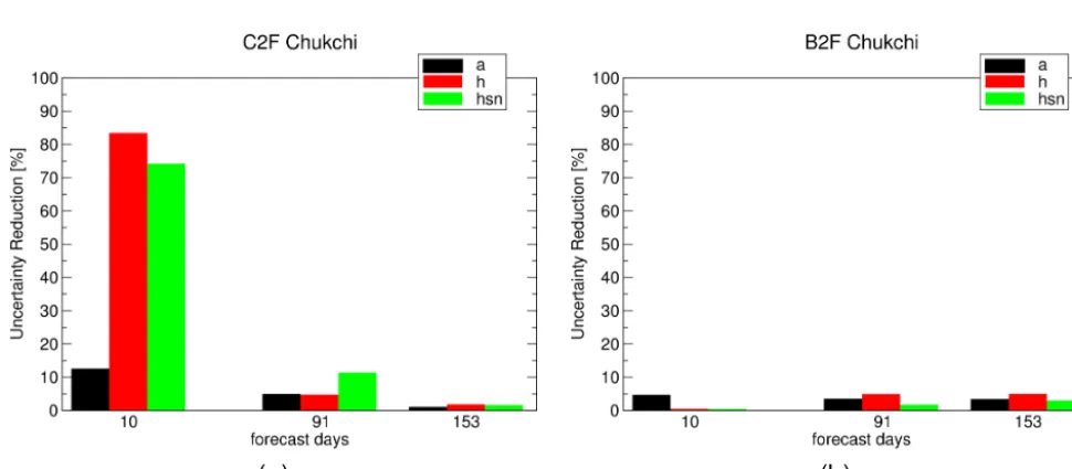
Figure 3. Uncertainty reduction for the Chukchi target area for flight transect C2F (a) and B2F (b) for target quantities mean ice concentration
a, mean ice thicknesshand mean snow depthhsn.
the lower bounds of airborne electromagnetic induction mea-surements (Haas et al., 2009).
4 Results and discussion
Figure 3 shows the performance of each transect in improv-ing forecasts over the Chukchi target region. We define the uncertainty reduction relative to the case without observa-tional constraints, where the prior uncertainty in the control vector (see Sect. 3.2) is propagated to the three target quan-tities. Overall we note a larger impact of C2F on the short-term forecast (10 days), while for B2F the impact increases for the mid-term forecast (3 months). For the mid-term fore-cast C2F surpasses B2F with respect to the impact on pre-dicted ice concentration and snow thickness, while its impact is marginally smaller for ice thickness. For the 10 day fore-cast C2F has a much larger impact on predicted ice and snow thickness than on ice concentration. This is mostly a result of the flights observing specifically the former two quantities, whereas the model dynamics require some time to transfer any constraints on snow and ice thickness into constraints on ice concentration. Moreover, ice concentration in this
re-gion is also strongly dependent on factors other than snow and ice thickness, in particular during spring and early sum-mer, when the role of wind forcing greatly exceeds that of the other two variables.
1728 T. Kaminski et al.: Evaluating Arctic sea ice thickness sampling strategies
Discussion
P
ap
er
|
Discussion
P
ap
er
|
Discussion
P
ap
er
|
Discussion
P
ap
er
|
(a)
(b)
Figure 4.
Sensitivity of target quantities over Chukchi area for 10 day (panel
a
), and 91
day
(panel
b
) forecasts to 1 sigma prior uncertainty change in each control variable. Units of target quantities
(and their sensitivities): ice concentration
(
a
)
(0–1); ice thickness
(
h
)
in m; snow thickness (hsn) in
m.
28
Figure 4. Sensitivity of target quantities over Chukchi area for 10-day (a) and 91-day (b) forecasts to 1 prior sigma uncertainty change in each control variable. Units of target quantities (and their sensitivities): ice concentration(a)(0–1); ice thickness(h)in metres; snow thickness (hsn) in metres.
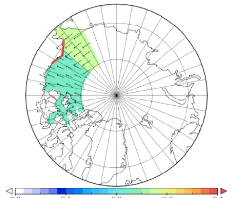
Figure 5. Wind stress direction with highest impact of tau com-ponent in control vector on ice thickness in Chukchi target region (dark red colour). Colour indicates magnitude.
two pieces of information: first, it shows the target direction; second, it shows the size of the impact of an uncertainty re-duction in the target direction. We note that the initial condi-tions of ice and snow have highest impact for the short-term forecast. For the mid-term forecast, atmospheric forcing and model parameters gain in importance. For the interpretation of the wind stress components taux and tauy recall that the model operates on a rotated coordinate system. Taking the rotation into account, for regions 6, 7, and 8 Fig. 5 shows the
direction in which a change of tau yields the largest increase in ice thickness. Adding a 25◦Ekman deflection, the change of ice motion is towards the target region. For the long-term forecast (153 days), the impacts (not shown) are generally small because there is little ice left in the target area. The impact of the B2F transect on the 10-day forecast of ice con-centration over the (remote) Chukchi target region (Fig. 3b) is remarkable. It is explained by the relatively high impact of the lead closing parameterh0in the formulation of freezing (control variable #89) on ice concentration (Fig. 4). Sinceh0 is a global parameter, observations on both transects can help to reduce uncertainty in this parameter.
Figure 6 shows the performance of each transect for im-proving forecasts for the target region covering the coastal ocean from Bering Strait to Prudhoe Bay (BS2PB). They show similar performance because this target quantity is tem-porally averaged from May to August. B2F is superior for snow thickness, and C2F for ice thickness and area. This can be explained by the sensitivity of these three target quantities (Fig. 7). Relative to ice thickness and area, snow thickness has a larger sensitivity to the initial (ice and snow) conditions (in particular over region 8) than to the surface forcing and the process parameters. And the initial snow thickness over region 8 is, of course, better observed by B2F (which crosses this region) than by C2F. As an additional test case we evalu-ate the combination of the two transects, which clearly shows their complementarity.
Figure 6. Uncertainty reduction for target area BS2PB for flight transects C2F, B2F, and both.
Figure 7. Sensitivity of target quantities for BS2PB area to 1 prior sigma uncertainty change in each control variable. Units of target quantities (and their sensitivities): ice concentration(a)(0–1); ice thickness(h)in metres; snow thickness (hsn) in metres.
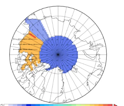
the largest increase in ice thickness. Adding a 25◦Ekman de-flection (to the right) the change of ice motion is towards the intersection of the respective region’s coastline with the target area BS2PB. The parameter pstar has a positive im-pact because it yields more rigid ice. Parameter h0, which essentially determines the distribution of newly formed ice in the vertical vs. the horizontal dimension, has a negative impact: increasing h0 yields thicker newly formed ice and consequently reduces the ice concentration.
Figure 9 shows the performance of each transect for im-proving forecasts over the NOB target region. The perfor-mance of B2F is much better than that of C2F for both
fore-Figure 8. Wind stress direction with highest impact of tau compo-nent in control vector on ice thickness in BS2PB target region (dark red colour). Colour indicates magnitude.
Discussion
P
ap
er
|
Discussion
P
ap
er
|
Discussion
P
ap
er
|
Discussion
P
ap
er
|
(a) (b)
Figure 9.Uncertainty reduction for target areas NOB for flight transect C2F (panela) and B2F (panel
b).
33
Figure 9. Uncertainty reduction for target areas NOB for flight tran-sect C2F (panel a) and B2F (panel b).
cast times. This result appears counter-intuitive, because C2F is much closer than B2F, but can be explained through the influence of the westward circulation prevailing in the wa-ters off the Alaskan coast (Eicken and Mahoney, 2015). For forecast times of 4–5 months, an upstream observation is as-sociated with much more predictive skill than an observation directly over the target area. In fact the same mechanism ex-plains the previously mentioned higher uncertainty reduction of B2F for the long-term forecast in the Chukchi area. For the target area BS2PB none of the transects dominate be-cause the target period is an integral from forecast months 2 to 5.
melt-1730 T. Kaminski et al.: Evaluating Arctic sea ice thickness sampling strategies
Discussion
P
ap
er
|
Discussion
P
ap
er
|
Discussion
P
ap
er
|
Discussion
P
ap
er
|
(a)
(b)
Figure 10.
Sensitivity of target quantity over NOB area for 132
day
(panel
a
), and 153
day
(panel
b
)
forecasts to 1 sigma prior uncertainty change in each control variable. Units of target quantities (and
their sensitivities): ice concentration
(
a
)
(0–1); ice thickness
(
h
)
in m; snow thickness (hsn) in m.
34
Figure 10. Sensitivity of target quantity over NOB area for 132-day (a) and 153-day (b) forecasts to 1 prior sigma uncertainty change in each control variable. Units of target quantities (and their sensitivities): ice concentration(a)(0–1); ice thickness(h)in metres; snow thickness (hsn) in metres.
Figure 11. Wind stress direction with highest impact of tau compo-nent in control vector on ice thickness in NOB target region (dark red colour). Colour indicates magnitude.
ing ice, albm, and the ice strength parameter, pstar) and the ice initial conditions.
There is generally little difference in the responses for the two forecast periods. This is an indication of the robustness of our linearisation of the coupled sea ice–ocean system and confirms an analysis of Kauker et al. (2009), who found, for the same model, moderate differences between the lineari-sation and finite size perturbations. A consequence of this robustness is that the specific target days we chose only play the role of a typical day within a longer time period.
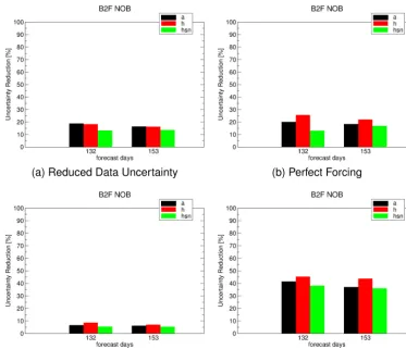
Figure 12 shows the sensitivity of the performance of the (superior) B2F transect with respect to changes in various impact factors (relative to the default settings used for Fig. 9) for the NOB target region. The reduction in data uncertainty from 0.3 to 0.1 m for both ice and snow thickness yields a considerable improvement in performance (panel a). The effect is particularly pronounced for ice area. Reducing the prior uncertainty for the atmospheric forcing to zero mimics the availability of a perfect seasonal atmospheric forecast. Under this assumption, the performance of the B2F transect is strongly increased (panel b). Likewise a reduction of the prior uncertainty for all process parameters mimics a per-fectly calibrated model. Its effect on the performance of the B2F transect is relatively small (panel c). Interestingly, com-bining the perfectly calibrated model and the perfect atmo-spheric forecast assumptions doubles the uncertainty reduc-tions compared to the perfect atmospheric forecast assump-tions alone. In this case all the observational constraints can fully act to reduce uncertainty in the initial conditions.
5 Conclusions
rep-P
ap
er
|
Discussion
P
ap
er
|
Discussion
P
ap
er
|
Discussion
P
ap
er
|
(a) Reduced Data Uncertainty (b) Perfect Forcing
(c) Perfect Model (d) Perfect Model and Forcing
Figure 12.Uncertainty reduction for target areas NOB for flight transect B2F with data uncertainty of 0.1m(panela), the assumption of perfectly known atmospheric forcing (panelb), the assumption of a perfectly calibrated model (panelc), the assumption of perfectly known atmospheric forcing and of a perfectly calibrated model (paneld).
36
Figure 12. Uncertainty reduction for target areas NOB for flight transect B2F with data uncertainty of 0.1 m (a), the assumption of perfectly known atmospheric forcing (b), the assumption of a perfectly calibrated model (c), the assumption of perfectly known atmospheric forcing and of a perfectly calibrated model (d).
resentative of future ice conditions in a rapidly changing Arc-tic.
Since our quantitative results are specific to the conditions in this particular year, we focus on overarching conclusions that can be drawn from this case study. First, we note that the network performance depends on the specific question asked, i.e. on the target quantity. Of equal importance in the highly advective Arctic sea ice regime is the finding that the longer the forecast time, the further upstream we have to sample, well outside of the region of interest. This may result in sig-nificant interannual variability in the area that needs to be targeted for measurements relative to the region of interest. This finding also supports the broader notion of an adaptive sampling grid that reflects a priori knowledge of the state and dynamics of the ice cover at the end of the ice growth season. On another level, we furthermore demonstrated in a quantita-tive way how the model dynamics transfer the observational information from one set of variables (snow depth and ice thickness) to another variable (ice concentration). In this con-text, we note that in our case study the target quantities and framework for assessing the QND were based on the specific objective of predicting summer ice conditions or navigation
along a heavily trafficked route in the Alaskan Arctic at the seasonal scale. Future work will have to evaluate the degree of overlap in uncertainty reduction for predictions on sea-sonal as compared to interannual or multidecadal timescales. When defining candidate networks to be evaluated, it is essential to take logistic constraints into account. The se-lection of alternate flight routes for the C2F and B2F tran-sects inherently reflects logistic factors. However, the QND approach lends itself to inclusion of quantitative constraints on specific regional data acquisition patterns that may re-quire further work to evaluate. Similarly, an essential input to the tool is the data uncertainty, which is the combination of uncertainties in the observations and in modelling their counterparts (model uncertainty). Hence, the QND approach can also help in evaluating methodological improvements or evaluate the costs/benefits of advances in instrumental design that reduce measurement errors. These findings make it clear that a QND tool needs to be operated by a team consisting of observationalists and modellers in order to derive maximum benefits.
1732 T. Kaminski et al.: Evaluating Arctic sea ice thickness sampling strategies specific model that is used. As long as the response
func-tions of our model are approximately correct, we can use the present system to simulate the observational impact on an assimilation system around a different model. For QND results to be valid beyond the model at hand, one has to em-ploy a well-validated model that includes all relevant pro-cesses. For example the model should have adequate sensi-tivity of regionally integrated ice properties with respect to the initial ice thickness. For the model used here this sen-sitivity is similar for resolutions from 1/2 to 1/12 of a de-gree. One would not expect a drastic change of this sensitiv-ity when moving to even finer (eddy-permitting) scales, but this requires further investigation. Computationally, the cur-rent 126-dimension control space requires 127 model sim-ulations (over 5 months each) for the approximation of the Jacobian matrices (M0of Eq. 3 andN0of Eq. 4) quantifying observational and target sensitivities. This should be feasible even for high-resolution models.
The current AOND system has the flexibility to also evalu-ate the potential of space missions or further in situ sampling strategies. There are a number of obvious ways to refine the present system. It can be extended to cover climate condi-tions over longer timescales and further into the future, possi-bly also representative of the state of the Arctic under climate change scenario for mid-century and beyond. Moreover, one could add oceanic observations or further target quantities, or extend the control vector to gain broader insights into observ-ing system design in the coupled atmosphere–sea ice–ocean system. Furthermore, rather than operating Arctic-wide, the same concept can be applied on a smaller regional scale when the forecasting period is short enough to ensure that the main influence factors can be appropriately simulated within the model domain.
Acknowledgements. This work has been funded by the European Commission through its Seventh Framework Programme Research and Technological Development under contract number 265863 (ACCESS) through a grant to FastOpt and OASys and by the National Science Foundation as part of the Sea Ice Prediction Network (SIPN) under grant number PLR-1304315. The authors thank two anonymous reviewers and Christian Haas for valuable comments on the manuscript.
Edited by: C. Haas
References
Barnett, D. G.: A practical method of long-range ice forecasting for the north coast of Alaska, Part I, Technical Report TR-1, Fleet Weather Facility, Suitland, Maryland, 1976.
Brubaker, M., Berner, J., Chavan, R., and Warren, J.: Climate change and health effects in Northwest Alaska, Glob. Health Ac-tion, 4, 8445, doi:10.3402/gha.v4i0.8445 2011.
Castro-Morales, K., Kauker, F., Losch, M., Hendricks, S., Riemann-Campe, K., and Gerdes, R.: Sensitivity of simulated Arctic sea
ice to realistic ice thickness distributions and snow parameteri-zations, J. Geophys. Res., 119, 559–571, 2014.
Crisp, D., Atlas, R., Breon, F.-M., Brown, L., Burrows, J., Ciais, P., Connor, B., Doney, S., Fung, I., Jacob, D., Miller, C., O’Brien, D., Pawson, S., Randerson, J., Rayner, P., Salaw-itch, R., Sander, S., Sen, B., Stephens, G., Tans, P., Toon, G., Wennberg, P., Wofsy, S., Yung, Y., Kuang, Z., Chudasama, B., Sprague, G., Weiss, B., Pollock, R., Kenyon, D., and Schroll, S.: The Orbiting Carbon Observatory (OCO) mission. Trace con-stituents in the troposphere and lower stratosphere, Adv. Space Res., 34, 700–709, 2004.
Drobot, S.: Long-range statistical forecasting of ice severity in the Beaufort-Chukchi Sea, Weather Forecast., 18, 1161–1176, 2003. Eicken, H.: Arctic sea ice needs better forecasts, Nature, 497, 431–
433, 2013.
Eicken, H. and Mahoney, A. R.: Sea ice: hazards, risks and impli-cations for disasters, in: Coastal and Marine Hazards, Risks, and Disasters, edited by: Ellis, J. and Sherman, D., Elsevier, Oxford, 381–401, 2015.
Giering, R. and Kaminski, T.: Recipes for adjoint code construction, ACM T. Math. Software, 24, 437–474, 1998.
Haas, C., Lobach, J., Hendricks, S., Rabenstein, L., and Pfaf-fling, A.: Helicopter-borne measurements of sea ice thickness, using a small and lightweight, digital EM system, J. Appl. Geo-phys., 67, 234–241, 2009.
Hardt, M. and Scherbaum, F.: The design of optimum networks for aftershock recordings, Geophys. J. Int., 117, 716–726, 1994. Hibler, W.: A dynamic thermodynamic sea ice model, J. Geophys.
Res., 9, 815–846, 1979.
Hibler, W. I. and Bryan, K.: A diagnostic ice-ocean model, J. Phys. Oceanogr., 17, 987–1015, 1987.
Kadygrov, N., Maksyutov, S., Eguchi, N., Aoki, T., Nakazawa, T., Yokota, T., and Inoue, G.: Role of simulated GOSAT to-tal column CO2 observations in surface CO2 flux uncer-tainty reduction, J. Geophys. Res.-Atmos., 114, D21208, doi:10.1029/2008JD011597, 2009.
Kalnay, E., Kanamitsu, M., Kistler, R., Collins, W., Deaven, D., Gandin, L., Iredell, M., Saha, S., White, G., Woollen, J., Zhu, Y., Chelliah, M., Ebisuzaki, W., Higgins, W., Janowiak, J., Mo, K. C., Ropelewski, C., Wang, J., Leetmaa, A., Reynolds, R., Jenne, R., and Joseph, D.: The NCEP/NCAR 40-year reanalysis project, B. Am. Meteorol. Soc., 77, 437–471, 1996.
Kaminski, T. and Rayner, P. J.: Assimilation and network design, in: Observing the Continental Scale Greenhouse Gas Balance of Europe, edited by: Dolman, H., Freibauer, A., and Valentini, R., Ecological Studies, chap. 3, Springer-Verlag, New York, 2008. Kaminski, T., Scholze, M., and Houweling, S.: Quantifying the
ben-efit of A-SCOPE data for reducing uncertainties in terrestrial car-bon fluxes in CCDAS, Tellus B, 62, 784–796, 2010.
Kaminski, T., Rayner, P. J., Voßbeck, M., Scholze, M., and Koffi, E.: Observing the continental-scale carbon balance: assessment of sampling complementarity and redundancy in a terrestrial as-similation system by means of quantitative network design, At-mos. Chem. Phys., 12, 7867–7879, doi:10.5194/acp-12-7867-2012, 2012.
Geo-phys. Res.-Oceans, 108, C63182, doi:10.1029/2002JC001573, 2003.
Kauker, F., Kaminski, T., Karcher, M., Giering, R., Gerdes, R., and Voßbeck, M.: Adjoint analysis of the 2007 all time Arctic sea-ice minimum, Geophys. Res. Lett.„ 36, L03707, doi:10.1029/2008GL036323, 2009.
Kauker, F., Gerdes, R., Karcher, M., Kaminski, T., Giering, R., and Voßbeck, M.: June 2010 Sea Ice Outlook – AWI/FastOpt/OASys, Sea Ice Outlook web page, available at: http://www.arcus.org/ search/seaiceoutlook/index.php (last access: 17 March 2015), 2010.
Köberle, C. and Gerdes, R.: Mechanisms determining the variability 2003: mechanisms determining the variability of Arctic sea ice conditions and export, J. Climate, 16, 2843–2858, 2003. Kurtz, N. T., Richter-Menge, J., Farrell, S., Studinger, M., Paden, J.,
Sonntag, J., and Yungel, J.: IceBridge Airborne Survey Data Sup-port Arctic Sea Ice Predictions, EOS T. Am. Geophys. Un., 94, p. 41, doi:10.1002/2013eo040001, 2013a.
Kurtz, N. T., Farrell, S. L., Studinger, M., Galin, N., Harbeck, J. P., Lindsay, R., Onana, V. D., Panzer, B., and Sonntag, J. G.: Sea ice thickness, freeboard, and snow depth products from Oper-ation IceBridge airborne data, The Cryosphere, 7, 1035–1056, doi:10.5194/tc-7-1035-2013, 2013b.
Lindsay, R., Haas, C., Hendricks, S., Hunkeler, P., Kurtz, N., Paden, J., Panzer, B., Sonntag, J., Yungel, J., and Zhang, J.: Seasonal forecasts of Arctic sea ice initialized with obser-vations of ice thickness, Geophys. Res. Lett., 39, L21502, doi:10.1029/2012GL053576, 2012.
Nickless, A., Ziehn, T., Rayner, P.J., Scholes, R.J., and Engel-brecht, F.: Greenhouse gas network design using backward La-grangian particle dispersion modelling – Part 2: Sensitivity anal-yses and South African test case, Atmos. Chem. Phys., 15, 2051– 2069, doi:10.5194/acp-15-2051-2015, 2015.
O’Brien, D. M. and Rayner, P. J.: Global observations of the carbon budget, 2, CO2column from differential absorption of reflected sunlight in the 1.61 µm band of CO2, J. Geophys. Res.-Atmos., 107, ACH 6-1–ACH 6-16, doi:10.1029/2001JD000617, 2002. Parkinson, C. and Washington, W.: A large-scale numerical model
of sea ice, J. Geophys. Res., 84, 311–337, 1979.
Patra, P. K., Maksyutov, S., Sasano, Y., Nakajima, H., Inoue, G., and Nakazawa, T.: An evaluation of CO2observations with So-lar occultation FTS for inclined-orbit satellite sensor for sur-face source inversion, J. Geophys. Res.-Atmos., 108, 4759, doi:10.1029/2003JD003661, 2003.
Rayner, P. J. and O’Brien, D. M.: The utility of remotely sensed CO2concentration data in surface source inversions, Geophys. Res. Lett., 28, 175–178, 2001.
Rayner, P. J., Enting, I. G., and Trudinger, C. M.: Optimizing the CO2observing network for constraining sources and sinks, Tel-lus B, 48, 433–444, 1996.
Rayner, P. J., Law, R. M., O’Brien, D. M., Butler, T. M., and Dil-ley, A. C.: Global observations of the carbon budget 3. Initial assessment of the impact of satellite orbit, scan geometry, and cloud on measuring CO2from space, J. Geophys. Res.-Atmos., 107, ACH 2-1–ACH 2-7, doi:10.1029/2001JD000618, 2002. Rayner, P. J., Utembe, S. R., and Crowell, S.: Constraining
re-gional greenhouse gas emissions using geostationary concentra-tion measurements: a theoretical study, Atmos. Meas. Tech., 7, 3285–3293, doi:10.5194/amt-7-3285-2014, 2014.
Richter-Menge, J. A. and Farrell, S. L.: Arctic Sea Ice Conditions in Spring 2009–2013 Prior to Melt, Geophys. Res. Lett., 40, 5888– 5893, 2013.
Richter-Menge, J. A. and Walsh, J. E. (Eds.): Seasonal-to-Decadal Predictions of Arctic Sea Ice: Challenges and Strategies, Na-tional Academies Press, Washington, DC, 2012.
Robards, M., Burns, J., Meek, C., and Watson, A.: Limitations of an optimum sustainable population or potential biological removal approach for conserving marine mammals: Pacific walrus case study, J. Environ. Manage., 91, 57–66, 2013.
Steele, M., Morley, R., and Ermold, W.: PHC: a global ocean hydrography with a high-quality Arctic ocean, J. Climate, 14, 2079–2087, 2001.
Stevens, D.: On open boundary condition in the united Kingdom Fine-Resolution Antarctic Model, J. Geophys. Res., 21, 1494– 1499, 1991.
Sumata, H., Kauker, F., Gerdes, R., Köberle, C., and Karcher, M.: A comparison between gradient descent and stochastic approaches for parameter optimization of a sea ice model, Ocean Sci., 9, 609–630, doi:10.5194/os-9-609-2013, 2013.