Y. Li1,2, G. Kirchengast3,2, B. Scherllin-Pirscher3, R. Norman2, Y. B. Yuan1, J. Fritzer3, M. Schwaerz3, and K. Zhang2 1State Key Laboratory of Geodesy and Earth’s Dynamics, Institute of Geodesy and Geophysics (IGG),
Chinese Academy of Sciences, Wuhan, China
2Satellite Positioning for Atmosphere, Climate, and Environment (SPACE) Research Centre, RMIT University, Melbourne, Victoria, Australia
3Wegener Center for Climate and Global Change (WEGC) and Institute for Geophysics, Astrophysics, and Meteorology/Institute of Physics, University of Graz, Graz, Austria
Correspondence to: Y. Li ([email protected])
Received: 1 November 2014 – Published in Atmos. Meas. Tech. Discuss.: 22 January 2015 Revised: 14 July 2015 – Accepted: 27 July 2015 – Published: 25 August 2015
Abstract. We introduce a new dynamic statistical optimiza-tion algorithm to initialize ionosphere-corrected bending an-gles of Global Navigation Satellite System (GNSS)-based ra-dio occultation (RO) measurements. The new algorithm esti-mates background and observation error covariance matrices with geographically varying uncertainty profiles and realistic global-mean correlation matrices. The error covariance ma-trices estimated by the new approach are more accurate and realistic than in simplified existing approaches and can there-fore be used in statistical optimization to provide optimal bending angle profiles for high-altitude initialization of the subsequent Abel transform retrieval of refractivity. The new algorithm is evaluated against the existing Wegener Center Occultation Processing System version 5.6 (OPSv5.6) algo-rithm, using simulated data on two test days from January and July 2008 and real observed CHAllenging Minisatel-lite Payload (CHAMP) and Constellation Observing System for Meteorology, Ionosphere, and Climate (COSMIC) mea-surements from the complete months of January and July 2008. The following is achieved for the new method’s per-formance compared to OPSv5.6: (1) significant reduction of random errors (standard deviations) of optimized bending angles down to about half of their size or more; (2) reduc-tion of the systematic differences in optimized bending an-gles for simulated MetOp data; (3) improved retrieval of re-fractivity and temperature profiles; and (4) realistically esti-mated global-mean correlation matrices and realistic uncer-tainty fields for the background and observations. Overall
the results indicate high suitability for employing the new dynamic approach in the processing of long-term RO data into a reference climate record, leading to well-characterized and high-quality atmospheric profiles over the entire strato-sphere.
1 Introduction
Global Navigation Satellite System (GNSS)-based radio oc-cultation (RO) is a robust atmospheric remote-sensing tech-nique that provides accurate atmospheric profiles of the Earth’s atmosphere (Kursinski et al., 1997; Hajj et al., 2002; Kirchengast, 2004). This technique has several distinctive ad-vantages in terms of high accuracy, high vertical resolution, global coverage, and self-calibration (Anthes, 2011; Yu et al., 2014). GNSS RO data are now widely used in numerical weather prediction, climate monitoring, and space weather research (e.g., Healy and Eyre, 2000; Cucurull and Derber, 2008; Le Marshall et al., 2010; Anthes, 2011; Steiner et al., 2011; Carter et al., 2013).
accuracy of the retrieved temperature and other atmospheric profiles (Healy, 2001; Rieder and Kirchengast, 2001; Gob-iet and Kirchengast, 2004; Steiner and Kirchengast, 2005). Therefore, it is very important to have a best-possible initial-ization of the ionosphere-corrected bending angles at high altitudes for more accurate climate monitoring.
Statistical optimization is a commonly used method to ini-tialize RO bending angles at high altitudes (e.g., Sokolovskiy and Hunt, 1996; Gorbunov et al., 1996; Hocke, 1997; Healy, 2001; Gorbunov, 2002; Gobiet and Kirchengast, 2004; Go-biet et al., 2007). It is a generalized least-squares approach that combines an observed RO bending angle profile with a background bending angle profile (Turchin and Nozik, 1969; Rodgers, 1976, 2000). The weights of the two types of bend-ing angles are determined by the inverse of their error co-variance matrices. The statistical optimization equation used is (Healy, 2001; Gobiet and Kirchengast, 2004)
αs=αb+Cb(Cb+Co)−1·(αo−αb) , (1) whereαsis the statistically optimized bending angle,αband αo are the respective (unbiased) background and observed bending angle profiles, and Cband Coare the corresponding error covariance matrices.
In statistical optimization, the more accurately the error covariance matrices represent the error characteristics, the more accurate is the optimized bending angle profile. How-ever, it is not straightforward to obtain such suitable error covariance matrices, especially for the background bending angle since they are not supplied together with common cli-matological models nor is the construction a straightforward task. Therefore, previous approaches have usually simplified the calculation of the error covariance matrices.
A typical approach is to estimate the background error covariance matrix by assuming a constant relative standard error of the background bending angle and a simple error correlation structure like exponential fall-off over an atmo-spheric scale height (Healy, 2001; Rieder and Kirchengast, 2001; Gobiet and Kirchengast, 2004) or disregarding correla-tions (Sokolovskiy and Hunt, 1996; Hocke, 1997; Gorbunov, 2002; Lohmann, 2005; Gorbunov et al., 1996, 2005, 2006). Similarly, the observation error covariance matrix is formu-lated from estimating the observation error at a defined meso-spheric altitude range (where the RO signal is weak) and using simple exponential fall-off error correlations (Healy, 2001, Gobiet and Kirchengast, 2004) or again just ignoring the latter. These rough estimations generally result in rate error covariance matrices and therefore result in inaccu-rate optimized bending angles that degrade the accuracy of subsequently retrieved atmospheric profiles. More details on the various schemes are provided by Li et al. (2013), Sect. 2.1 therein.
Improved accuracy in optimized bending angles was ob-tained when using an improved statistical optimization algo-rithm to initialize ionosphere-corrected bending angles (Li,
2013; Li et al., 2013). Li et al. (2013) used European Cen-tre for Medium-Range Weather Forecasts (ECMWF) short-range (24 h) forecast fields as background bending angles. Their background error covariance matrix was accurately and realistically estimated using large ensembles of ECMWF short-range forecast, analysis, and RO observed bending an-gles. It was constructed using daily global fields of estimated background uncertainty profiles and a daily global-mean cor-relation matrix. The background uncertainty profile was dy-namically estimated taking into account its variations with latitude, longitude, altitude, and day of year. They not only calculated the random errors of background bending angles using large ensembles of ECMWF and RO data but also em-pirically modeled the potential systematic background uncer-tainty and finally combined these two uncertainties to formu-late the background uncertainty. The global-mean correlation matrix was also calculated using large ensembles of ECMWF analysis and forecast fields. Finally, the biases in the back-ground bending angles were corrected to avoid the potential effects on optimized bending angles.
Since this first-version dynamic statistical optimization al-gorithm dynamically estimated the background error covari-ance matrix only, it is hereafter referred to as the b-dynamic algorithm (“b” represents background) in this study. The b-dynamic algorithm was evaluated by Li et al. (2013) against the Occultation Processing System version 5.4 (OPSv5.4) al-gorithm developed by the Wegener Center for Climate and Global Change (WEGC) (Pirscher, 2010; Ho et al., 2012; Steiner et al., 2013). It was found that the b-dynamic algo-rithm significantly reduced random errors of the optimized bending angles and left less or about equal levels of residual systematic errors. The quality of the subsequently retrieved refractivity and temperature profiles was also improved. In addition, even the dynamically estimated background error correlation matrix alone was able to improve the optimized bending angles.
Fi-cludes two parts: (1) the dynamic estimation of the back-ground error covariance matrix and the bias correction of background bending angles, and (2) the dynamic estima-tion of the observaestima-tion error covariance matrix. Informa-tion on background/observaInforma-tion uncertainty and on the back-ground/observation correlation matrix is needed for con-structing complete background/observation error covariance matrices. The uncertainty at any vertical level is the square root of the diagonal value of the error covariance matrix at that level. The correlation matrix includes correlation func-tions for all vertical levels. Each such correlation function comprises the correlation coefficients of the error at the ver-tical level where it peaks to the errors at all other verver-tical levels. In summary, the background/observation uncertain-ties and the corresponding correlation matrix together for-mulate the background/observation error covariance matrices (Gaspari and Cohn, 1999).
Assuming thatk=1,. . . ,Noccare sequentially numbered RO events of a day, then for each occultation eventkthe dy-namic algorithm estimates the (unbiased) background bend-ing angle profileαkb and its corresponding error covariance matrix Ckb, as well as the observation error covariance matrix Cko. Using these three quantities together with the observed bending angleαko, the statistically optimized bending angle profileαks can be determined as
αsk=αbk+CbkCkb+Cko
−1 ·
αok−αkb
. (2)
The algorithm for the estimation ofαbkand Ckbhas been de-scribed in detail by Li et al. (2013) as part of the b-dynamic algorithm. It will be briefly summarized in Sect. 2.1, focusing on the key algorithmic steps and the advances in the dynamic algorithm. In Sect. 2.2, details on the computation of Ckoand other issues that are critical to the capability of the dynamic algorithm are provided.
2.1 Dynamic estimation of the background error covariance matrix and bias calibration of background bending angles
The dynamic estimation of the background error covariance matrix includes three algorithmic steps: (1) construction of
algorithm, which used 200 representative impact altitude lev-els from 0.1 km to 80.0 km with non-equidistant spacing, this new scheme allows direct use of these variables for the next step of calculation, avoiding additional vertical interpolation of all variables and particularly also within correlation matri-ces.
The data used to calculate these basic background vari-ables include ECMWF analysis fields and corresponding 24 h forecast fields with a T42L91 resolution at 00:00 and 12:00 UTC, and observed RO bending angles. In calculating the mean variables in each grid cell, time averaging over 7 days (from 3 days before to 3 days after the day of interest) and horizontal averaging over geographic domains of at least 1000 km×3000 km (over 10◦latitude×60◦longitude cells from 60◦S to 60◦N, poleward over larger longitude ranges of 95◦from 60 to 70◦N/S, 120◦from 70 to 80◦N/S, and 270◦ from 80 to 90◦N/S) were used. Compared to the b-dynamic scheme, which used 5 days of data only and smaller geo-graphic regions (1000 km×1000 km) for averaging, this up-date allows more data to be used for more reliable statistical estimates (especially important for mean observed bending angles) at each 10◦latitude×20◦longitude grid point, while still capturing the slow variations of the mean field well. These calculations include mean variables, the construction of error correlation matrices, and empirical modeling of bi-ases. For details see Li et al. (2013).
The second step involves the preparation of the derived daily background fields. These specific statistical quantities include (i) the forecast-minus-analysis standard deviations sf−a, which represent the estimated random uncertainty of the background bending angles; (ii) the estimated uncertainty of the mean background bending angleub; and (iii) the differ-ence between the mean forecast bending angle and the mean background bending angle1α¯f−b.
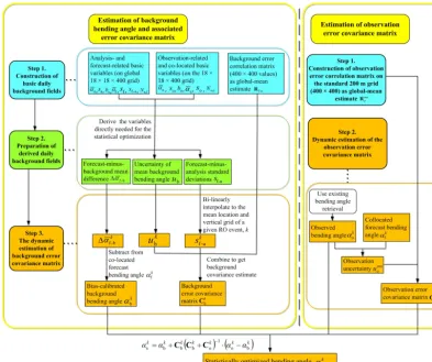
Figure 1. Schematic illustration of the algorithmic steps of the dynamic statistical optimization approach; for description see Sect. 2.1 and 2.2.
uoccb =
fbc·ukb 2
+sfk−a2 1/2
. (3)
Herein the bias coverage factor fbcis introduced as a user-defined parameter that can be employed to penalize the es-timated bias-type uncertainty ukb relative to the estimated random uncertainty sfk−a. This enables minimizing the in-fluence from potential residual background biases, relative to observation uncertainty, on the resulting optimized pro-file αsk. In this study the bias coverage factor was chosen to linearly decrease with altitude, settingfbc=15 at 30 km (strong penalty in lower stratosphere) and fbc=1 at 80 km (no penalty at top boundary). This choice was found to be useful for climate applications (more discussion of fbc, in-cluding for comparison also example cases with constant fbc=1 andfbc=5, is given in Sect. 3.2). Using the back-ground standard uncertainty and the global-mean correlation matrix Rf−a=Rf−a,ij, the background error covariance ma-trix Ckb=Cbk,ijis formulated as
Ckb,ij=uoccb,i ·uoccb,j·Rf−a,ij. (4)
In order to effectively reduce the residual bias in the back-ground bending angleαbk (cf. Eq. 2) to within the estimated uncertainty of the background meanukb,αkbis calculated by subtracting the forecast-minus-background mean difference 1α¯fk−bfrom the co-located forecast bending angleαfk: αbk=αfk−1α¯fk−b. (5)
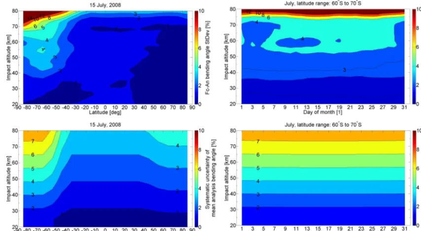
Figure 2 illustrates the estimated relative uncertainty of the forecast-minus-analysis standard deviation 100·(sf−a/α¯a) (top) and the modeled relative systematic bias of the ECMWF analysis bending angle 100·(ba/α¯a)(bottom).ba is the main component ofukb (cf. Li et al., 2013) andα¯a is the ECMWF analysis mean bending angle;ba therefore il-lustrates the size of the systematic uncertainty termfbc·ukb in Eq. (3) when fbc=1, i.e., when no user-defined bias penalty is employed. Any application of a bias coverage fac-torfbc>1, such as used in this study for representing climate-quality retrievals, magnifies this term accordingly.
Figure 2. Variability of relative standard deviations of forecast-minus-analysis bending angle differences (upper two panels) and of the systematic uncertainty of the mean analysis bending angle (bottom two panels) as function of latitude (left) and of day of month (right), respectively.
and to∼3 % at 50 km, and remain at∼1 % below 25 km. In non-polar regions, the standard deviations amount approxi-mately to 3 to 4 % near 80 km, decrease to 2 % at 75 km and remain within 1 to 2 % below. The day-to-day temporal evo-lution ofsf−aat high southern latitudes (60 to 70◦S) (right) reveals relatively smooth uncertainty conditions for the en-tire month of July, without much temporal dynamics in the uncertainty. In the course of testing, it was found that the es-timates are consistent with flow-dependent forecast-minus-analysis error estimates produced by ECMWF’s Ensemble of Data Assimilations (EDA) system (Isaksen et al., 2010; Bonavita et al., 2011; M. Bonavita, ECMWF, personal com-munication, 2012).
Regarding variations of 100·(ba/α¯a)as a function of lati-tude (bottom left), the bias-type uncertainties are also largest at high altitudes in the Southern Hemisphere. The relative un-certainties are larger than 7 % near 80 km, decreasing to 5 % at 60 km, and remain smaller than 3 % below 40 km. In non-polar regions, the relative uncertainties amount to 4 % near 80 km, decreasing to below 2 % also at 40 km. The temporal evolution of the systematic uncertainty 100·(ba/α¯a)over a month (bottom right) shows that these relative uncertainties also reveal little sub-monthly variations, due to the way in which they are constructed (Li et al., 2013).
Figure 3 shows exemplary global-mean correlation func-tions (left) and associated correlation lengths (right) for the 5, 15, and 25 July 2008. The correlation functions, plotted for three representative height levels (30, 50, 70 km), are rather similar over the month. They have a main peak of
Figure 3. Global-mean error correlation functions from the back-ground error covariance matrix (left), for the 5, 15, and 25 July 2008 at three representative impact altitude levels (30, 50, and 70 km), and estimated correlation lengths of the correlation functions (right) at all impact altitude levels from 20 to 80 km for the same 3 days.
nearly Gaussian shape with negative side peaks at each side. Further outward, small secondary positive peaks occur, af-ter which the functions essentially approach zero. The cor-relation lengths increase rather smoothly with altitude from about 0.8 km at 20 km to 6 km at 80 km. They also show little variation over the example month of July 2008.
daily update of the background fields was used as a cautious baseline.
2.2 Dynamic estimation of the observation error covariance matrix
The error covariance matrix of the observed bending an-gleCok is calculated using an observation uncertainty profile uocco , estimated on a per-event basis, and a global-mean error correlation matrix Rocco :
Cok=uocco,iuocco,jRoocc,ij. (6) Different to the OPSv5.6 and the b-dynamic algorithm, which estimate the observation uncertainty uocco between about 65 and 80 km with an MSIS climatology model bend-ing angle profile as a reference (Li et al., 2013), the full dynamic algorithm estimates uocco as a vertical profile over the stratopause region and mesosphere, using the co-located ECMWF forecast bending angle profile as a reference.
More specifically, the first step is to subtract the co-located forecast bending angle profileαkf from the observed bending angle profileαko:
1αok=αok−αfk. (7)
The difference profile1αokis then smoothed with a 15 km window moving average (from 45 km to the top bound of the profile, usually 80 km). The resulting smoothed differ-ence profile is denoted as1αko.
The next step is to subtract the smoothed difference profile 1αkofrom the original difference profile1αkoin order to ob-tain a delta-difference profile11αokthat essentially contains only random errors:
11αok=1αok−1αko. (8) Finally the observation uncertainty at any impact altitude level i (corresponding to the impact altitude ofzi)of each occultation event,uocco,i, is calculated as
uocco,i =
v u u t
1 n−1
iz+7.5
X
n=iz−7.5
11αk
o,n 2
, (9)
wherenis the number of sample points betweenzi+7.5 km andzi−7.5 km and whereiz−7.5andiz+7.5denote the cor-responding impact altitude indices. Equation (9) is applied from 45 km to the top of the profile, providing uocco,i esti-mates from 52.5 to 72.5 km; below (above) the value at 52.5 km (72.5 km) is extended downward (upward) just as a constant value. This construction ensures that variations over the mesosphere can be accounted for while data below the stratopause, where the estimated delta-difference profile 11αok may also contain atmospheric variability noise (e.g., from gravity wave activity), are not allowed to influence the estimate.
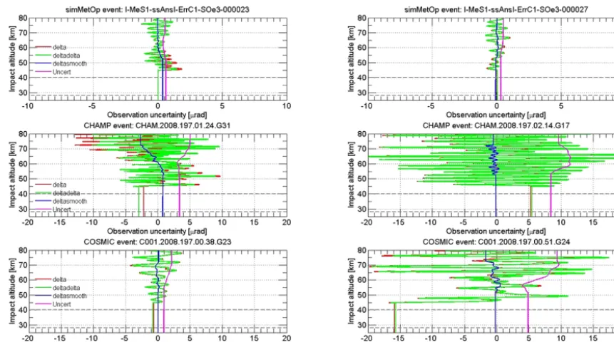
Figure 4 illustrates the observation uncertainty profile uocco , and intermediate variables from Eqs. (7) and (8), for six example RO events from 15 July 2008. The simMetOp events are simulated using the End-to-end GNSS Occulta-tion Performance SimulaOcculta-tion and Processing System soft-ware version v5.6 (EGOPSv5.6) in the same way as the sim-MetOp ensemble was produced by Li et al. (2013); for more details see Sect. 3 below. In each panel, the red line shows the original difference profile1αok(“delta”), the blue line the smoothed difference profile1αko(“deltasmooth”), the green line the delta-difference profile11αok(“deltadelta”), and the magenta line the observation uncertaintyuocco (“Uncert”). It can be seen that Eqs. (7) and (8) are robust in removing sys-tematic errors, leaving a good random signal, from which the uncertaintyuocco is reliably estimated.
Estimated uncertainties are smallest (near 0.5 µrad) for the simMetOp events (top) that mimic MetOp/GRAS-type high performance receiver errors without additional noise effects (Li et al., 2013) and are distinctively larger for real data from CHAMP (middle) and COSMIC (bottom). The uncertain-ties of CHAMP and COSMIC bending angles can be quite variable, as illustrated, and can reach 10 µrad or more for CHAMP events, while it is typically only around 2 µrad or so for COSMIC. Figure 4 also shows that the variation of uncer-tainty, which often may come from variations in ionospheric small-scale noise being added onto the RO receiver-related noise, can be well captured over the mesosphere.
The global-mean observation error correlation matrix Rocco is estimated using the difference profiles between the ob-served and co-located ECMWF analysis bending angle pro-files. In this estimation, we first construct a global-mean error covariance matrix using all available difference profiles from 3 days before to 3 days after the day of interest, i.e., using the same weekly smoother as for the background estimations. Then we derive the global-mean correlation matrix by divid-ing all elements of the covariance matrix by their correspond-ing square roots of diagonal values. RO observations used for this calculation included data from COSMIC and GRACE for January and July 2008, and MetOp-A for July 2008 (no processed data were available for January 2008). The ob-tained error correlation matrix Rocco is used based on Eq. (6) for the construction of the observation error covariance ma-trices Cko, for all RO eventskof the day. We did not include a bias calibration step similar to the background bias calibra-tion (Eq. 5) at the observacalibra-tion side. Such a step may com-plement the Cko estimation in the future, however, for sub-tracting residual ionospheric biases in the observed bending angle profilesαko before they enter the calculation of mean observed bending angles (as part of estimating1α¯fk−b; Li et al., 2013) and the statistical optimization equation (Eq. 2).
Figure 4. Observation uncertainty and key intermediate variables for six representative RO events, two simMetOp events (top), two CHAMP events (middle), and two COSMIC events (bottom) from 15 July 2008. “delta” is the difference profile of the RO ionosphere-corrected bending angle to the co-located ECMWF forecast profile used as a reference, “deltadelta” is the delta-difference profile after subtracting a smoothed profile “deltasmooth” from the difference profile “delta”, and “Uncert” is the resulting observation uncertainty estimate; for detailed description see Sect. 2.2.
Figure 5. Global-mean error correlation functions from the obser-vation error covariance matrix (left), for the 5, 15, and 25 July 2008 at three representative impact altitude levels (30, 50, and 70 km), and estimated correlation lengths of the correlation functions (right) at all impact altitude levels from 20 to 80 km for the same 3 days. For ease of intercomparison the layout is the same as in Fig. 3.
of the different characteristics. By comparing Figs. 3 and 5, it can be seen that the observation error correlation functions are basically similar in shape to the background error correla-tion funccorrela-tions (main peak, negative side peaks, smaller pos-itive secondary side peaks) albeit with significantly shorter correlation lengths. In addition, the functional shape of side peaks is not as smooth as the one for the background. The correlation length is essentially constant with altitude (above 30 km), amounting to about 0.8 km.
The intra-monthly variation is essentially negligible within the given July 2008 test month (applies also to January 2008,
not shown), pointing to room for further improvement of the utility of the estimation for long-term processing, e.g., con-sidering larger ensemble sizes and sub-global regions. These slow dynamics of the observation error covariance matrices, and of the background error covariance matrices as discussed in Sect. 2.1, enable reliable use also in near-real-time or fast-track processing (i.e., processing within 3 h or within follow-on day of observatifollow-ons). Instead of using 7 days centered about the day being processed (including 3 days before and after the center day) 7-day-history data (from the previous day to 7 days prior) may be used in these cases, with in-significant degradation in performance.
2.3 Other improvements of the new algorithm
background uncertainties. In order to safeguard against these effects, we have improved the algorithm as follows.
First, we gracefully adjust the observation uncertaintyuo computed according to Sect. 2.2 based on adjusting the observation-to-background uncertainty ratio robu=uo/ub below 40 km, in order to ensure that it approaches a robust small value at the bottom of the statistical optimization range. We modify therobuprofile to make it linearly transit from the robu value prevailing at 40 km torobu=0.1 at 28 km. Typ-ical values within 28 and 40 km may range from near 0.1 (simMetOp) to around 1 (CHAMP), so the linear transit to 0.1 at 28 km generally implies a decrease of therobufor real data. In order to avoid any possible sharp change of therobu profile at 40 km, we smooth the resulting profile by a mov-ing average filter with 2 km width. Usmov-ing the modified robu profile, the observation uncertainty is then reconstructed as uo(zi)=robu(zi)·ub(zi), enforcing dominance of the obser-vation information in the optimized profile from 40 km to 28 km. Alternatively to this uo(zi)adjustment used in this study, the background uncertainty profile may be adjusted, ub(zi)=uo(zi)/robu(zi), which keeps the effect on the opti-mized profile the same while leaving the observation uncer-tainty unchanged.
Second, we apply the statistical optimization down to 28 km and then apply a half-sine-weighted transition across 32 to 28 km between the statistically optimized bending an-gles and purely observed bending anan-gles. That is, the weight-ing function over this transition altitude range,w(zi), is for-mulated as
w (zi)=0.5·
sin π
2 ·
zi−zsoT 1zsoT
+1
, (10)
wherezsoTis the statistically optimized-to-observed bending angle transition altitude, set to 30 km, and1zsoTis the statis-tically optimized-to-observed bending angle transition half width, set to 2 km. Employingw(zi)from 32 to 28 km in the form
αsoT(zi)=w (zi)·αs(zi)+(1−w (zi))·αo(zi) , (11) we get a well-defined gradual transition from optimized bending angle to observed bending angle. When these two improvements to the b-dynamic algorithm are applied, the sometimes “spiky” behavior of some (CHAMP) profiles near the bottom boundary of statistical optimization discussed by Li et al. (2013) disappeared.
Another issue requiring caution is the robustness of ma-trix inversions, especially related to the weighting mama-trix in Eq. (2), Cb(Cb+Co)−1, containing the inversion of the sum-mary matrix of the observation and background error covari-ance matrices. Since the observation error correlation func-tions can be insufficiently smooth and since the main peaks are close to Gaussian shape, the summary matrix can become close to ill-conditioned and cannot be accurately inverted in this case, inducing undue noise into the resulting weighting matrix.
This could be overcome by replacing the main peak by a 5th-order polynomial function as described by Gaspari and Cohn (1999), which approximates a Gaussian shape and was also successfully used in the context of matrix inversion by Steiner and Kirchengast (2005), Eq. (5) therein (note that a typo leaked into thez2term as cited in this equation forz< 1; the correct denominator is “3” instead of “2”, as in thez2 term cited for the 1 <zbranch). After using this approxima-tion, the inversion was sufficiently robust. Alternatives for ensuring robustness include the use of even-larger ensemble sizes in matrix construction and more advanced methods of matrix inversion such as truncated singular value decompo-sition.
3 Evaluation of the new dynamic statistical optimization algorithm
The dynamic algorithm was implemented in the EGOPSv5.6 software (Fritzer et al., 2013) to enable a complete RO re-trieval. The EGOPSv5.6 system was also used to simu-late RO observations (simMetOp events) and to retrieve at-mospheric profiles. The standard RO data processing chain within this system is the OPSv5.6 retrieval.
We evaluated the new dynamic algorithm against this OPSv5.6 algorithm, which is, in terms of statistical optimiza-tion formulaoptimiza-tion, the same as the OPSv5.4 algorithm used for comparison by Li et al. (2013). Briefly, the OPSv5.6 al-gorithm uses ECMWF short-range forecast bending angles as a background and employs exponential fall-off functions to express the correlations of both background and observa-tion uncertainties. The background uncertainty is modeled as amounting to 15 % of background bending angles. The ob-servation uncertainty is estimated as the standard deviation of observed bending angles relative to co-located MSIS model bending angles in the impact altitude range from 65 km to about 80 km. For more detailed information on OPSv5.6/v5.4 see Pirscher (2010), Steiner et al. (2013), and Schwaerz et al. (2013).
In addition to the OPSv5.6 intercomparison, the atmo-spheric profiles retrieved by the dynamic algorithm are com-pared with those retrieved by the b-dynamic algorithm (Li et al., 2013) and with those by the UCAR/COSMIC Data Anal-ysis and Archive Center (CDAAC) Boulder.
The data sets used for the evaluation include simulated MetOp data (simMetOp) as well as real observed CHAMP and COSMIC data. simMetOp data were simulated in the same way as by Li et al. (2013), using moderate ionosphere conditions in the forward simulations and using observa-tional errors representing MetOp/GRAS-type receiving sys-tem errors.
were used as a reference. This is the same setup as was used by Li et al. (2013).
3.1 Algorithm performance for individual profiles
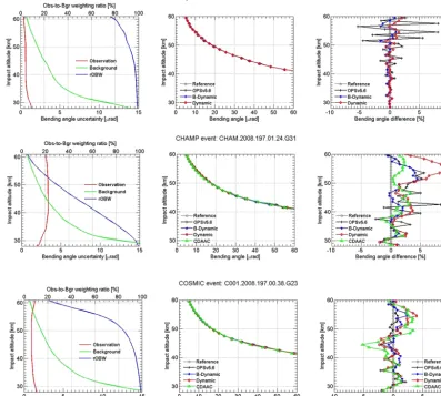
Figure 6 illustrates the effects of statistical optimization on individual bending angle profiles by a few representative RO events. The left panels show the background and observation uncertainties as well as the observation-to-background (Obs-to-Bgr) weighting ratio robw=100·ub2/(u2b+u2o), which expresses on a percentage scale how the information is weighted between observations and background. robw is a convenient approximate variable for this purpose, which ex-actly applies if the covariance matrices in the statistical op-timization equation (Eq. 2) are diagonal. Observation un-certainty is smallest for the simMetOp event (top), largest for the CHAMP event (middle), and in between for the COSMIC event (bottom). At 60 km these observation un-certainties are roughly 0.4, 3, and 1.5 µrad for simMetOp, CHAMP, and COSMIC, respectively. These differences in observation uncertainty yield the largest robw for the sim-MetOp event and the smallest for CHAMP. Related to this, the altitude where both observations and background re-ceive equal weight (robw=50 %), which may be consid-ered the transition altitude below which the observation in-formation dominates the retrieval, is highest for simMetOp (> 60 km), medium for COSMIC (around 55 km), and small-est for CHAMP (near 45 km). Ongoing follow-on work on large RO data sets of many months analyzes therobw statisti-cally and confirms that these few example events are typical for the respective data sources.
Since bending angles increase roughly exponentially with decreasing altitude, as seen in the middle column of Fig. 6, differences among the various retrieved profiles seem to be small. The right panels, however, actually show the differ-ences of optimized bending angle profiles relative to their reference. For the simMetOp event, bending angle differ-ences from the dynamic algorithm are smallest over all al-titudes, confirming the high utility of the algorithm, since here the “true” profile from forward simulation serves as a reference. The bending angle differences of the b-dynamic algorithm are similar and the values are also small. The
dif-Inspecting further individual RO events (not shown) con-firmed that the relative differences of simMetOp data from the dynamic algorithm are consistently smaller and smoother than those from the other approaches. This underlines the robust capability of the dynamic algorithm for improving the quality of the ionosphere-corrected bending angles. For CHAMP and COSMIC measurements, the relative differ-ences from the dynamic algorithm are also generally smaller and smoother than those from other algorithms below 50 km. However, above 50 km, the differences from both the dy-namic algorithm and from CDAAC are generally larger than those from the OPSv5.6 and b-dynamic approaches. This does not mean that bending angle profiles from the dynamic and CDAAC algorithms are not accurate at high altitudes, however; the result mainly depends on the determination of the weights of the background and observed bending angles in the statistical optimization.
ob-Figure 6. Background and observation bending angle uncertainty profiles as well as observation-to-background (Obs-to-Bgr) weighting ratio (left); statistically optimized bending angle profiles from the OPSv5.6, b-dynamic, dynamic, and CDAAC algorithms together with their reference profile (middle); and difference of the optimized profiles to the reference profile (right). Three example events from 15 July 2008 are illustrated, from simMetOp (top), CHAMP (middle), and COSMIC (bottom), respectively.
servation as used in the OPSv5.6 formulation. The dynami-cally estimated uncertainties were used for both cases since we are interested only in the differences from the correlations in this particular test.
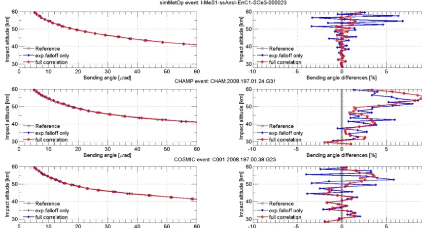
Figure 7 shows the comparison results for these two types of correlation matrices, again using three exemplary events from simMetOp, CHAMP, and COSMIC, showing absolute bending angles (left) and differences to reference (right). The simMetOp event highlights that bending angle differences from the full correlation case are much smoother and smaller than those from the exponential fall-off correlation. For the real CHAMP and COSMIC events, the magnitudes of the differences from the two cases are similar, but also here it is clearly evident that the use of the full correlation leads to smoother differences than the use of exponential fall-off correlation. We conclude that the use of adequately realistic correlation matrices is preferable.
3.2 Statistical performance evaluation results
In this section the performance of the dynamic, b-dynamic, and OPSv5.6 statistical optimization algorithms are evalu-ated using simulevalu-ated MetOp data from 15 January and 15 July 2008 and monthly CHAMP and COSMIC observations from January and July 2008. In addition, atmospheric pro-files retrieved and provided by UCAR/CDAAC for the same time periods are used for comparison. The mean systematic differences between retrieved and reference profiles and the associated standard deviations are calculated and analyzed in bending angle, refractivity, and temperature profiles, similar to the statistical performance evaluation of the b-dynamic al-gorithm by Li et al. (2013).
Figure 7. Statistically optimized bending angle profiles together with their reference profile (left) and their difference to the reference profile (right), of three example events from simMetOp (top), CHAMP (middle), and COSMIC (bottom) from 15 July 2008, using either the realistic global-mean correlation matrix of the new dynamic method (“full correlation”) or simple exponential fall-off correlation as existing in OPSv5.6 (“exp.falloff only”).
exceeds a threshold at any impact altitude level, which was defined based on careful sensitivity tests as the maximum of either 40 µrad absolute or 25 % relative deviation from the co-located ECMWF short-range forecast bending angle. In practice, looking at it from the top downwards, the transi-tion from the absolute to the relative criterion occurs roughly around 35 km, where bending angle values start to exceed 160 µrad.
Refractivity and temperature profiles are checked in the same way as used for OPSv5.6/v5.4 (Schwaerz et al., 2013; Steiner et al., 2013; Pirscher, 2010), i.e., the deviation from co-located ECMWF analysis profiles at any altitude level must not exceed 10 % for refractivity between 5 and 35 km and 20 K for temperature within 8 and 25 km. These qual-ity checks are performed on all profiles retrieved with the EGOPS software. For profiles provided by CDAAC, we check the CDAAC quality flag and use only profiles flagged to be of good quality.
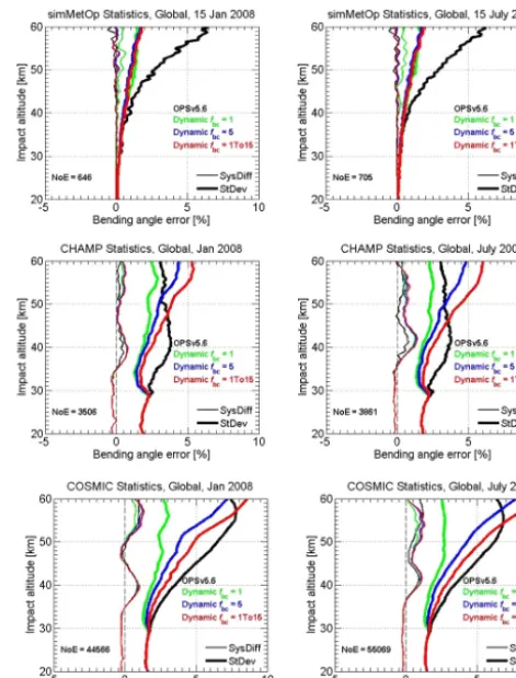
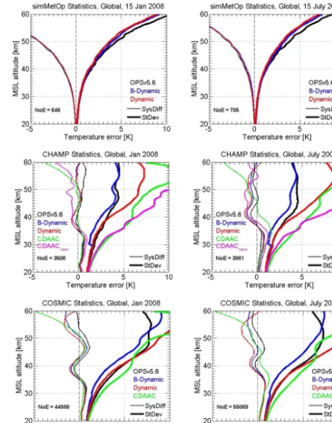
Figure 8 shows the systematic differences and standard de-viations of optimized bending angle profiles of the global en-sembles of simMetOp from 15 January and 15 July 2008, and of CHAMP and COSMIC events from January and July 2008. For simMetOp (top), it is clear to see that the perfor-mance of the dynamic algorithm outperforms the b-dynamic algorithm and the OPSv5.6 algorithm, exhibiting smallest systematic differences and associated standard deviations. Compared to the OPSv5.6 algorithm, the best improvement is found between 40 and 60 km. These results are very
en-couraging and confirm the fundamental capabilities of the dynamic algorithm.
Comparison of the CHAMP (middle) and COSMIC (bot-tom) results from the dynamic algorithm with the OPSv5.6 and CDAAC algorithms shows that the bending angle stan-dard deviation from the dynamic (and b-dynamic) algorithm is again generally smaller than that of the OPSv5.6 and CDAAC results. Above 45 km for CHAMP, and above 55 km for COSMIC, the standard deviations from the dynamic al-gorithm exceed those from the OPSv5.6 alal-gorithm. This is due to increased weight of noisy RO bending angles in the mesosphere compared to OPSv5.6 as discussed in Sect. 3.1 above. Standard deviations from both CDAAC data versions are larger than those from the other methods, and particularly the new data version (shown for CHAMP) exhibits largest standard deviation already from about 35 km upwards.
Figure 8. Systematic differences (SysDiff, light lines) and standard deviations (SD, heavy lines) of statistically optimized bending an-gles, relative to “perfect” simulated bending angles or co-located ECMWF analysis bending angles used as a reference, of the global ensemble of simMetOp events on 15 January and 15 July 2008 (up-per two panels), and of CHAMP and COSMIC events from the com-plete months of January and July 2008 (middle and bottom panel, respectively). Statistics of the OPSv5.6 (black), b-dynamic (blue), dynamic (red), CDAAC (version 2009.2650 for CHAMP and ver-sion 2010.2640 for COSMIC, green), and CDAACnew (version 2014.0140 for CHAMP, magenta) statistical optimization methods are shown. The number of events (NoE) used in the ensemble of each statistical calculation is also indicated in each panel.
expected from its realistic account for both observation and background uncertainties and error correlation structures.
Furthermore it can be seen, in particular from the CHAMP results (CHAMP data have highest observational noise), that the improved treatment of the transition to purely observed data around 30 km has mitigated the sharpness of the change in standard deviation.
In order to discuss the effects of different choices offbc on the resulting optimized bending angles, we compared the choice of this study for linear altitude dependence (see Sect. 2.1; termedfbc=1 To 15 here) with the choice in the algorithmic introduction by Li et al. (2013) (fbc=5) and with a reference case intentionally making no use of the bias penalty option (fbc=1). Figure 9 shows the comparative
re-Figure 9. Systematic differences (SysDiff, light lines) and standard deviations (SD, heavy lines) of statistically optimized bending an-gles, relative to “perfect” simulated bending angles or co-located ECMWF analysis bending angles used as a reference, of the global ensemble of simMetOp events on 15 January and 15 July 2008 (up-per two panels), and of CHAMP and COSMIC events from the complete months of January and July 2008 (middle and bottom pan-els, respectively). Results from three different bias coverage factor choices in the dynamic algorithm – i.e.,fbc=1 (green),fbc=5 (blue), andfbc=1 To 15 (red) – as well as from the OPSv5.6 algo-rithm (black) are shown.
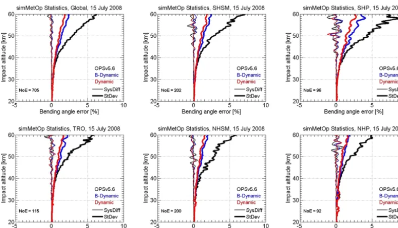
Figure 10. Systematic differences (SysDiff, light lines) and standard deviations (SD, heavy lines) of statistically optimized bending angles, relative to “perfect” simulated bending angles used as a reference, of simMetOp events on 15 July 2008. Statistics for the OPSv5.6 (black), b-dynamic (blue), and dynamic (red) statistical optimization algorithms are shown for six different regions: Global (90◦S to 90◦N), TRO (tropics, 20◦S to 20◦N), SHSM (Southern Hemisphere subtropics and midlatitudes, 20 to 60◦S), NHSM (Northern Hemisphere subtropics and midlatitudes, 20 to 60◦N), SHP (Southern Hemisphere polar region, 60 to 90◦S), and NHP (Northern Hemisphere polar region, 60 to 90◦N). The number of events (NoE) used in the ensemble of each region is also indicated in the panels.
For the CHAMP and COSMIC data, standard deviations are largest for thefbc=1 To 15 case, medium for thefbc=5 case, and smallest for the fbc=1 case. This is in line with the expectation of how therobwchanges under these different choices since the observational noise is more and more miti-gated the more relative weight the background receives. The effect on the systematic differences (for CHAMP and COS-MIC relative to the co-located ECMWF analysis profiles) is relatively small in these global-scale statistics; but also here the direction is that no bias penalty forces the results towards the background mean state at high altitudes.
Overall Fig. 9 demonstrates that the sensitivity to the de-tailed quantitative choice offbcis fairly weak, as can be seen from the moderate differences between these three cases with very differentfbcchoices. This is favorable since it implies that no detailed quantitative tuning offbcis needed in prac-tice; thefbcas the only free user-defined variable in the new dynamic algorithm is rather a clear and transparent option to predefine the influence of background information according to what users deem suitable for their application.
In order to evaluate the performance of different statisti-cal optimization algorithms in different latitude regions, the systematic differences and standard deviations of optimized bending angles were calculated for five latitudinal bands in addition to the global case (90◦S to 90◦N), including trop-ics (TRO, 20◦S to 20◦N), Southern Hemisphere/Northern Hemisphere subtropics and midlatitudes (SHSM/NHSM,
20◦S/N to 60◦S/N), and Southern Hemisphere/Northern Hemisphere polar regions (SHP/NHP, 60◦S/N to 90◦S/N). Figures 10, 11, and 12 show the statistical results for the global case (for context, same as in right column of Fig. 8) and for these five regions for simMetOp (Fig. 10), CHAMP (Fig. 11), and COSMIC (Fig. 12). The July 2008 results are shown, which are found to be well representative; the latitude-resolved data characteristics in January 2008 are similar.
Figure 10 shows that the performance of the dynamic, b-dynamic, and OPSv5.6 algorithms are rather similar glob-ally and in the Northern Hemisphere (NHSM, NHP). In the Southern Hemisphere, and in particular in the SHP region (Antarctic winter in July), the conditions are evidently more challenging, such that the OPSv5.6 algorithm accrues in-creased biases in the upper stratosphere above 50 km. The new dynamic algorithm underscores its good and reliable ba-sic performance in all regions, both in terms of biases and standard deviations.
Figure 11. Systematic differences (SysDiff, light lines) and standard deviations (SD, heavy lines) of statistically optimized bending angles, relative to co-located ECMWF analysis bending angles used as a reference, of CHAMP events from July 2008. Statistics for the OPSv5.6 (black), b-dynamic (blue), dynamic (red), CDAAC (version 2009.2650, green), and CDAACnew(version 2014.014, magenta) statistical optimization algorithms are shown for the same six regions as in Fig. 10. The figure layout is the same as for Fig. 10.
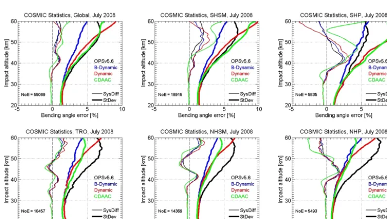
Figure 12. Systematic differences (SysDiff, light lines) and standard deviations (SD, heavy lines) of statistically optimized bending angles, relative to co-located ECMWF analysis bending angles used as a reference, of COSMIC events from July 2008. Statistics for the OPSv5.6 (black), b-dynamic (blue), dynamic (red), and CDAAC (version 2010.2640, green) statistical optimization algorithms are shown for the same six regions as in Fig. 10. The figure layout is the same as for Figs. 10 and 11.
at altitudes above 35 km (up to around 5 %) and also stan-dard deviations closely reaching or exceeding 10 % even at altitudes near 50 km. Error characteristics for January (not shown) in the NHP region (Arctic winter) generally mirror the SHP July (Antarctic winter) error characteristics.
Figure 13. Systematic differences (SysDiff, light lines) and stan-dard deviations (SD, heavy lines) of retrieved refractivity profiles, relative to “perfect” simulated refractivity or co-located ECMWF analysis refractivity used as a reference, for the global ensemble of simMetOp events on 15 January and 15 July 2008 (top panels) and of CHAMP events (middle panels) and COSMIC events (bot-tom panels) from the complete months of January and July 2008. Statistics of the OPSv5.6 (black), b-dynamic (blue), dynamic (red), CDAAC (version 2009.2650 for CHAMP and version 2010.2640 for COSMIC, green), and CDAACnew (version 2014.0140 for CHAMP, magenta) statistical optimization methods are shown. The figure layout is the same as for Fig. 8.
will also include stricter validation against independent co-located data of high quality over the stratosphere and meso-sphere from other sources such as the Envisat/MIPAS and TIMED/SABER satellite instruments (Remsberg et al., 2008; García-Comas et al., 2012).
Figures 13 and 14 show the global statistics results for re-fractivity (Fig. 13) and temperature (Fig. 14) for simMetOp (top), CHAMP (middle), and COSMIC (bottom). These re-fractivity and temperature results reflect the results for the bending angles in a filtered manner, after having passed through the Abelian integration (refractivity) and in addi-tion the hydrostatic integraaddi-tion (temperature), which lead to smoothing and downward propagation of biases and to re-duction of standard deviations (e.g., Gobiet and Kirchengast, 2004; Steiner and Kirchengast, 2005). Due to this downward
Figure 14. Systematic differences (SysDiff, light lines) and stan-dard deviations (SD, heavy lines) of retrieved temperature profiles, relative to “perfect” simulated temperature or co-located ECMWF analysis temperature used as a reference, for the global ensemble of simMetOp events on 15 January and 15 July 2008 (top panels) and of CHAMP events (middle panels) and COSMIC events (bottom panels) from the full months of January and July 2008. The figure layout is the same as for Figs. 8 and 13.
propagation, the differences from the various algorithms be-come smaller, and results are closely similar below about 40 km and in most cases even above. The most notable differ-ences from the consistent behavior of the different algorithms are those of the CDAAC processings above about 50 km, which exhibit the largest systematic differences and standard deviations, and the additional deviations of the new CDAAC version (shown for CHAMP) already from about 35 km up-wards.
Again we consider the performance of the new dynamic algorithm robust and encouraging for larger-scale applica-tions, which may also include further adjustments of param-eters likefbcand of averaging domains for constructing the dynamic uncertainty and correlation information.
Figure 15. Bending angle (left), refractivity (middle), and temperature (right) systematic differences (SysDiff, light lines) and standard deviations (SD, heavy lines), relative to their “perfect simulated” or co-located ECMWF analysis data used as a reference, of the global ensemble of simMetOp (top) and COSMIC (bottom) events from 15 July 2008, using either the realistic global-mean correlation matrix of the new dynamic method (“full correlation”) or simple exponential fall-off correlation as in the existing OPSv5.6 (“exp.falloff only”). The number of events (NoE) in each statistical ensemble is also indicated in the panels.
full dynamic algorithm or from using simplified correlation modeling with the exponential fall-off approximation. The simMetOp results show, in line with the results of Fig. 7, that the use of the realistically modeled full correlations is a superior choice, though the reduction of systematic differ-ence relative to the “true” referdiffer-ence is small (after the Abel or hydrostatic integrations) in refractivity and temperature. The COSMIC results indicate that the choice of correlation mod-eling strongly impacts the standard deviation and to a more limited degree also the systematic differences. While this be-havior does not itself imply a preference, it is very clear that the choice of the realistic full correlation modeling will be the physically more sound and more adequate approach also for real data.
4 Summary and conclusions
This study presented a new dynamic statistical optimization algorithm to initialize RO ionosphere-corrected bending an-gle profiles at high altitudes for optimal climate monitoring throughout the stratosphere. This dynamic algorithm uses multiple days of ECMWF analysis, ECMWF short-range (24 h) forecast, and RO observation data to realistically es-timate background and observation error covariance matri-ces. Both the background and observation error covariance matrices are constructed with geographically varying uncer-tainty estimation and with a global-mean correlation matrix estimated on a daily basis. The b-dynamic algorithm recently
introduced by Li et al. (2013) was used as a starting point and provided for the estimation of the background error covari-ance matrix and the bias correction of background bending angles.
The main advancements of the new dynamic algorithm compared to this previous algorithm are that it (1) adds a dy-namically estimated observation error covariance matrix with altitude-dependent observation uncertainty and a realistically calculated globmean correlation matrix; (2) updates the al-gorithm of the calculation of basic statistical mean variables by using ECMWF and RO data from a longer time window and larger geographical regions for more accurate and reli-able estimation; and (3) eliminates weaknesses that existed near the lower boundary of statistical optimization (30 km) by improving the uncertainty formulation and transition to purely observed data across this boundary.
ulated MetOp data on single days (15 January and 15 July 2008) and real observed CHAMP and COSMIC data from two full months (January and July 2008). The following was found for the new dynamic algorithm, in particular compared to OPSv5.6: (1) it can reduce systematic errors (biases) and standard deviations of optimized bending angles, as proven by simMetOp data including “true” reference profiles from end-to-end simulations, and subsequently also benefits the error characteristics of retrieved refractivity and temperature profiles; (2) it can reduce the random errors of optimized bending angles in the stratosphere for real data, as evaluated for CHAMP and COSMIC, still at the same time leaving less or about equal residual systematic error (bias) in the bending angles; (3) it can better account for the observational noise in the mesosphere, leading to larger standard deviations than OPSv5.6 there from greater weight of the observations in the optimized profiles, albeit without applying any artificial ob-servation uncertainty values in the case of high noise levels.
Beyond the evaluation of the new dynamic algorithm against OPSv5.6, atmospheric profiles from UCAR/CDAAC were also intercompared, including use of very recently re-leased CHAMP data from the newest (2014) CDAAC data version. It was found that CDAAC bending angles gener-ally exhibit markedly higher standard deviations above about 35 km and that in particular the new data version shows com-paratively large systematic differences and standard devia-tions. The reasons for this new-version behavior deserve fur-ther study.
Overall, compared to previous simplified approaches of statistical optimization, the dynamic algorithm presented here, which realistically estimates both background and ob-servation error covariance matrices, contains high capabili-ties for future large-scale implementation. The evaluation of the algorithm provided clear evidence that it can deliver re-liable and accurate atmospheric profiles for atmosphere and climate applications. The results therefore indicate high suit-ability for employing the new dynamic approach in the pro-cessing of long-term RO data into a climate record, leading to well-characterized and high-quality atmospheric profiles over the entire stratosphere.
project (AAS 4159) and the Australian Natural Disaster Resilience Grant Scheme (NDRG) of Victoria at the RMIT side; and the funding support by the European Space Agency (ESA) project OPSGRAS, the Austrian Research Promotion Agency (FFG) project OPSCLIMTRACE, and the Austrian National Science Fund (FWF) project DYNOCC (T620-N29) at the WEGC side.
Edited by: A. von Engeln
References
Anthes, R. A.: Exploring Earth’s atmosphere with radio occulta-tion: contributions to weather, climate and space weather, At-mos. Meas. Tech., 4, 1077–1103, doi:10.5194/amt-4-1077-2011, 2011.
Bassiri, S. and Hajj, G. A.: Higher-order ionospheric effects on the GPS observables and means of modeling them, Manuscr. Geod., 18, 280–289, 1993.
Bonavita, M., Raynaud, L, and Isaksen, L.: Estimating back-ground error variances with the ECMWF Ensemble of Data Assimilations system: Some effects of ensemble size and day-to-day variability, Q. J. Roy. Meteor. Soc., 137, 423–434, doi:10.1002/qj.756, 2011.
Carter, B. A., Zhang, K., Norman, R., Kumar, V. V., and Kumar, S.: On the occurrence of equatorial F-region irregularities during so-lar minimum using radio occultation measurements, J. Geophys. Res. Space Physics., 118, 892–904, doi:10.1002/jgra.50089, 2013.
Cucurull, L. and Derber, J. C.: Operational implementa-tion of COSMIC observaimplementa-tions into NCEP’s global data assimilation system, Wea. Forecasting., 23, 702–711, doi:10.1175/2008WAF2007070.1, 2008.
Danzer, J., Scherllin-Pirscher, B., and Foelsche, U.: Systematic residual ionospheric errors in radio occultation data and a poten-tial way to minimize them, Atmos. Meas. Tech., 6, 2169–2179, doi:10.5194/amt-6-2169-2013, 2013.
Fritzer, J., G. Kirchengast, G., and Pock, M.: End-to-End Generic Occultation Performance Simulation and Processing System version 5.6 (EGOPS 5.6) Software User Manual, Tech. Rep. ESA/ESTEC-1/2013, Wegener Center and Inst. for Geophys., Astrophys., and Meteorol., University of Graz, Graz, Austria, 505 pp., 2013.
López-González, M. J., and Schwartz, M. J.: On the quality of MIPAS kinetic temperature in the middle atmosphere, Atmos. Chem. Phys., 12, 6009–6039, doi:10.5194/acp-12-6009-2012, 2012.
Gaspari, G. and Cohn, S. E.: Construction of correlation functions in two and three dimensions, Q. J. Roy. Meteor. Soc., 125, 723– 757, doi:10.1002/qj.49712555417, 1999.
Gobiet, A. and Kirchengast, G.: Advancements of Global Navi-gation Satellite System radio occultation retrieval in the upper stratosphere for optimal climate monitoring utility, J. Geophys. Res., 109, D24110, doi:10.1029/2004JD005117, 2004.
Gobiet, A., Kirchengast, G., Manney, G. L., Borsche, M., Retscher, C., and Stiller, G.: Retrieval of temperature profiles from CHAMP for climate monitoring: intercomparison with Envisat MIPAS and GOMOS and different atmospheric analyses, At-mos. Chem. Phys., 7, 3519–3536, doi:10.5194/acp-7-3519-2007, 2007.
Gorbunov, M. E.: Ionospheric correction and statistical opti-mization of radio occultation data, Radio Sci., 37, 1084, doi:10.1029/2000RS002370, 2002.
Gorbunov, M. E., Gurvich, A. S., and Bengtsson, L.: Advanced al-gorithms of inversion of GPS/MET satellite data and their appli-cation to reconstruction of temperature and humidity, Report No. 211, Max-Planck-Institute for Meteorology, Hamburg, 46 pp., 1996.
Gorbunov, M. E., Lauritsen, K. B., Rhodin, A., Tomassini, M., and Kornblueh, L.: Analysis of the CHAMP experimental data on radio-occultation sounding of the Earth’s atmosphere, Izvestiya, Atmospheric and Oceanic Physics, 41, 726–740, 2005.
Gorbunov, M. E., Lauritsen, K. B., Rhodin, A., Tomassini, M., and Kornblueh, L.: Radio holographic filtering, error estimation, and quality control of radio occultation data, J. Geophys. Res.,111, D10105, doi:10.1029/2005JD006427, 2006.
Hajj, G. A., Kursinski, E. R., Romans, L. J., Bertiger, W. I., and Leroy, S. S.: A technical description of atmospheric sounding by GPS occultation, J. Atmos. Sol. Terr. Phys., 64, 451–469, doi:10.1016/S1364-6826(01)00114-6, 2002.
Healy, S. B.: Smoothing radio occultation bending angles above 40 km, Ann. Geophys., 19, 459–468, doi:10.5194/angeo-19-459-2001, 2001.
Healy, S. B. and Eyre, J. R.: Retrieving temperature, water vapour and surface pressure information from refractive-index profiles derived by radio occultation: A simulation study, Q. J. Roy. Me-teor. Soc., 126, 1661–1683, doi:10.1002/qj.49712656606, 2000. Hocke, K.: Inversion of GPS meteorology data, Ann. Geophys., 15,
443–450, doi:10.1007/s00585-997-0443-1, 1997.
Ho, S.-P., Hunt, D., Steiner, A. K., Mannucci, A. J., Kirchen-gast, G., Gleisner, H., Heise, S., von Engeln, A., Marquardt, C., Sokolovskiy, S., Schreiner, W., Scherllin-Pirscher, B., Ao, C., Wickert, J., Syndergaard, S., Lauritsen, K. B., Leroy, S., Kursin-ski, E. R., Kuo, Y-H., Foelsche, U., Schmidt, T., and Gorbunov, M.: Reproducibility of GPS radio occultation data for climate monitoring: Profile-to-profile inter-comparison of CHAMP cli-mate records 2002 to 2008 from six data centers, J. Geophys. Res., 117, D18111, doi:10.1029/2012JD017665, 2012.
Isaksen, L., Haseler, J., Buizza, R., and Leutbecher, M.: The new Ensemble of Data Assimilations, ECMWF Newsl, 123, 17–21, 2010.
Kirchengast, G.: Occultations for probing atmosphere and climate: Setting the scene, in: Occultations for Probing Atmosphere and Climate, edited by: Kirchengast, G., Foelsche, U., and Steiner, A. K., 1–8, Springer, Berlin-Heidelberg, 2004.
Kursinski, E. R., Hajj, G. A., Schofield, J. T., Linfield, R. P., and Hardy, K. R.: Observing Earth’s atmosphere with radio occulta-tion measurements using the Global Posiocculta-tioning System, J. Geo-phys. Res., 102, 23429–23465, doi:10.1029/97JD01569, 1997. Le Marshall, J., Xiao, Y., Norman, R., Zhang, K., Rea, A.,
Cucu-rull, L., Seecamp, R., Steinle, P., Puri, K., and Le, T.: The benefi-cial impact of radio occultation observations on Australian region forecasts, Aust. Meteorol. Oceanogr. J., 60, 121–125, 2010. Li, Y.: A new dynamic approach for the statistical optimization of
GNSS radio occultation bending angles (PhD thesis), RMIT Uni-versity, Melbourne, Australia, 141 pp., 2013.
Li, Y., Kirchengast, G., Scherllin-Pirscher, B., Wu, S., Schwaerz, M., Fritzer, J., Zhang, S., Carter, B. A., and Zhang, K.: A new dynamic approach for statistical optimization of GNSS radio oc-cultation bending angles for optimal climate monitoring utility, J. Geophys. Res., 118, 13022–13040, doi:10.1002/2013JD020763, 2013.
Liu, C. L., Kirchengast, G., Zhang, K. F., Norman, R., Li, Y., Zhang, S. C., Carter, B., Fritzer, J., Schwaerz, M., Choy, S. L., Wu, S. Q., and Tan, Z. X.: Characterisation of residual ionospheric errors in bending angles using GNSS RO end-to-end simulations, Adv. Space Res., 52, 821–836, doi:10.1016/j.asr.2013.05.021, 2013. Liu, C. L., Kirchengast, G., Zhang, K., Norman, R., Li, Y., Zhang, S.
C., Fritzer, J., Schwaerz, M., Wu, S. Q., and Tan, Z. X.: Quantify-ing residual ionospheric errors in GNSS radio occultation bend-ing angles based on ensembles of profiles from end-to-end simu-lations, Atmos. Meas. Tech., 8, 2999–3019, doi:10.5194/amt-8-2999-2015, 2015.
Lohmann, M. S.: Application of dynamical error estimation for sta-tistical optimization of radio occultation bending angles, Radio Sci., 40, RS3011, doi:10.1029/2004RS003117, 2005.
Manney, G. L., Daffer, W. H., Strawbridge, K. B., Walker, K. A., Boone, C. D., Bernath, P. F., Kerzenmacher, T., Schwartz, M. J., Strong, K., Sica, R. J., Krüger, K., Pumphrey, H. C., Lambert, A., Santee, M. L., Livesey, N. J., Remsberg, E. E., Mlynczak, M. G., and Russell III, J. R.: The high Arctic in extreme winters: vortex, temperature, and MLS and ACE-FTS trace gas evolution, Atmos. Chem. Phys., 8, 505–522, doi:10.5194/acp-8-505-2008, 2008. Pirscher, B.: Multi-satellite climatologies of fundamental
atmo-spheric variables from radio occultation and their validation (PhD thesis), Sci. Rep., 33–2010, Wegener Center Verlag Graz, Graz, Austria, 218 pp., 2010.
Remsberg, E. E., Marshall, B. T., Garcia-Comas, M., Krueger, D., Lingenfelser, G. S., Martin-Torres, J., Mlynczak, M. G., Russell III., J. M., Smith, A. K., Zhao, Y., Brown, C., Gordley, L. L., Lopez-Gonzalez, M. J., Lopez-Puertas, M., She, C.-Y., Taylor, M. J., and Thompson, R. E.: Assessment of the quality of the Ver-sion 1.07 temperature-versus-pressure profiles of the middle at-mosphere from TIMED/SABER, J. Geophys. Res. Atmos., 113, D17101, doi:10.1029/2008JD010013, 2008.
GPS/MET workshop, Union Radio Sci. Int., Tucson, Ariz., 1996. Steiner, A. K. and Kirchengast, G.: Error analysis for GNSS radio occultation data based on ensembles of profiles from end-to-end simulations, J. Geophys. Res., 110, D15307, doi:10.1029/2004JD005251, 2005.
tion of incorrectly posed problems, Izvestiya, Atmospheric and Oceanic Phys., Engl. Transl., 5, 14–18, 1969.