Nonlinear Processes in Geophysics (2002) 9: 367–371
Nonlinear Processes
in Geophysics
c
European Geophysical Society 2002
Numerical wind wave model with a dynamic boundary layer
V. G. Polnikov, Y. A. Volkov, and F. A. Pogarskii
A. M. Obukhov Institute for Atmospheric Physics of the Russian Academy of Sciences, Pyzhevskii lane, 3, 109017 Moscow, Russia
Received: 05 March 2001 – Revised: 23 July 2001 – Accepted: 22 January 2002
Abstract. A modern version of a numerical wind wave
model of the fourth generation is constructed for a case of deep water. The following specific terms of the model source function are used: (a) a new analytic parameterization of the nonlinear evolution term proposed recently in Zakharov and Pushkarev (1999); (b) a traditional input term added by the routine for an atmospheric boundary layer fitting to a wind wave state according to Makin and Kudryavtsev (1999); (c) a dissipative term of the second power in a wind wave spec-trum according to Polnikov (1991). The direct fetch testing results showed an adequate description of the main empiri-cal wave evolution effects. Besides, the model gives a cor-rect description of the boundary layer parameters’ evolution, depending on a wind wave stage of development. This per-mits one to give a physical treatment of the dependence men-tioned. These performances of the model allow one to use it both for application and for investigation aims in the task of the joint description of wind and wave fields.
1 Introduction
The problem of constructing an effective and physically well-grounded wind wave model is far from being solved. One reason for this circumstance dwells in the extreme complex-ity of the processes that take place at the air-sea interface and are responsible for the wind wave evolution. Therefore, de-spite progress in the scope gained over the last 10–15 years (see, for example, monographs Efimov and Polnikov, 1991; Komen et al., 1994; Lavrenov, 1998), some questions have been raised at present, which can be solved in order to con-struct a new generation model.
In realitiy, all known wind wave models incorporate, as a rule, empirical parameterization of the nonlinear evolution term with ambiguous fitting parameters (the SWAMP group, 1985; Komen et al., 1994). From the fundamental point of view, this fact is a weak link of any model. Additionally, all
Correspondence to: V. G. Polnikov ([email protected])
known models are constructed without a dynamic fitting of an air boundary layer to a state of wind waves (a dynamic boundary layer regime). At the same time, recent advances in the wind wave theory permit one to remove the principal drawbacks mentioned above in a wind wave model and to construct more elaborate models with a dynamic boundary layer. According to the project SWAMP (the SWAMP group, 1985) classification, such models could be attributed to the next fourth generation.
As a prototype of a new generation model, one may point to the spectral wind wave model presented in Zakharov et al. (1999). But due to the use in this model of the so-called “nar-row directional approximation”, the model is only applicable for narrow angular spread spectra. The use of this model for arbitrary, non-uniform wind fields needs a special basing.
The model proposed in this paper has significant differ-ences from the model of Zakharov et al. (1999). First, this model is based on the diffusive approximation for the exact nonlinear term, derived recently in Zakharov and Pushkarev (1999). This is the more universal approximation with re-spect to the one used in Zakharov et al. (1999). As shown in a special investigation (Polnikov, 2002), this approximation is applicable even in the case of mixed sea. Second, in our case, the more advanced model of a dynamic boundary layer proposed in Makin and Kudravtsev (1999) is used. Third, the square power in a wind wave spectra dissipation term is used in the model. Effectiveness of such a dissipation term is shown in Polnikov (1985, 1991), and the foundation of it is given in Polnikov (1994, 1995). Some experimental evi-dence of such a dissipation is given in Donelan (1998). All these elements of the new model warrant a priori a wider do-main of applicability with respect to all known models.
The most important new fields of applicability of the pro-posed numerical model are the following:
1. Investigation of the air-sea interaction physics;
3. Combination of the wind wave model with an atmo-sphere circulation model to provide changeable bound-ary conditions at the air-sea interface.
All other traditional fields of application described in mono-graphs mentioned above are available for the proposed wind wave model as well.
2 Main equations
The main evolution equation for the frequency-angle wind wave spectrum,S(σ, θ,x, t ), has the kind
∂S ∂t +Cgx
∂S ∂x +Cgy
∂S
∂y =F ≡N l+I n−Dis . (1)
Here,σ andθ represent the frequency and the angle of the wave component, respectively;xis the vector of the horizon-tal coordinates,tis the time variable,Cgx,Cgyare the group velocity components of the wave,Fis the source function in-cluding the following evolution mechanisms:N Lis the rate of conservative nonlinear energy transfer through the wave spectrum (“nonlinearity”);I nis the rate of energy transfer from the wind to the waves (“input”);Disis the rate of wave energy loss due to wave breaking and interaction with the upper layer turbulence (“dissipation”).
2.1 Nonlinear evolution mechanism
To describe the nonlinear evolution term of the model, we use the formula derived in Zakharov and Pushkarev (1999) in the diffusion approximation for the exact nonlinear kinetic integral. In the frequency-angle representation, this formula has the kind
N l(σ, θ )= ∂S(σ, θ ) ∂t
N L
=cg−4σ Lhσ12S3(σ, θ )i , (2) whereLis the differential operator of the second order
L= 1
2
∂2 ∂σ2+
1
σ2
∂2
∂θ2 . (3)
The difference from the original paper by Zakharov and Pushkarev (1999) is that the gravity acceleration constant,g, and the only fitting coefficient,c, are introduced here in the explicit form. As it was shown in a special study (Polnikov, 2002), the value ofcis of the order of 0.1.
2.2 Input mechanism
In the energy containing frequency domain ( 0.5σp ≤ σ ≤ 2.5σp, whereσp is the peak frequency), the input term has the traditional kind
I n=β(σ, θ,U)σ S(σ, θ ), (4)
and the growing increment,β, is given by the empirical for-mula ion (Snyder et al., 1981)
β(σ, θ,U)=max
0, aρa ρb
· 28U
∗σ
g cos(θ−θu)−b
(5)
Here, the following notions are used:ρaandρbrepresent the air and water density, respectively,U∗is the friction velocity,
andθu is the local wind direction. Parametersa andb are varying in the following intervals: a ∼=0.2−0.3 andb ∼=
0.9−1.
In the higher frequency domain σ > 2.5σp, the Plant’s parameterization forβis used (Plant, 1982)
β =(0.04±0.02)
U
∗σ
g 2
cos(θ−θu) . (6)
2.2.1 Dynamic boundary layer
A fitting of the air boundary layer to the sea state (a dynamic boundary layer regime) is realized by means of using a spe-cial procedure for calculating the friction velocity,U∗. For
this aim the new model of the boundary layer evolution over the sea surface is used (Makin and Kudryavtsev, 1999). The essence of this model is the following.
As usual, it is proposed that the total momentum flux to waves,τ, can be represented as a sum of the turbulent flux,
τt, and the wave-induced flux,τw:
τ ≡U∗2=τt+τw. (7)
Hereafter, the fluxτ is normalized to the air density for sim-plicity. Further, the turbulent flux is calculated by the use of the following equation for a turbulent shear layer
τt(z)=K∂U (z)
∂z . (8)
A use of the turbulent energy balance equation with some simplifications permitted Makin and Kudryavtsev to deter-mine an expression for the vertical eddy viscosity coefficient,
K. The latter allows one to solve Eq. (8) analytically and to write an explicit expression for the vertical wind velocity profile of the kind
U (z)=U∗2
z
Z
zv0
1−τ
w(z)
U2
∗
K−1dz
= U∗ κ
z
Z
zv0
1−τ
w(z)
U2
∗
34
d(lnz) . (9)
Here,z0vis the viscous sub-layer width the order of which is defined by the formulazv0 ∼=0.1 v
U∗t, wherevis the
kinemat-ical viscosity of the air, andU∗t is the turbulent part of the
friction velocity.
Thus, all boundary layer parameters, namely the friction velocity,U∗, the wind profile,U (z), and the drag coefficient,
V. G. Polnikov et al.: Numerical wind wave model with a dynamic boundary layer 369 latter, the following equation was derived
τw(z) U2
∗
=
σmax Z
σmin
dσ I
θ
dθ
1−τ
w(0)
U2
∗
·
exp(−10zk)cos(5π zk)R
c
U10
·k2S(σ, θ )cos(θ )|cos(θ )|
. (10)
Here,k = σ2
g is the wave number,R
c U10
is the empirical long-wave cutting factor for the Plant’s input term, a similar type to that given in Makin and Kudryavtsev (1999), c = g/σ is the phase velocity of the wave component, andU10is the known value of the wind velocity at the standard horizon,
z = 10 m. The limits of integration, σmin and σmax, are defined by the lower edge of the numerical frequency interval and by a specially chosen upper limit for the high frequency spectrum tail, respectively.
Thus, the problem of estimation of the friction velocity,
U∗, the drag coefficient,C10, and the effective value of the roughness parameter, z0ef, becomes closed for the given valueU10and the known sea state. Note that in order to find the effective roughness,z0ef, one should take a hypotheses of the profileU (z). In our estimations, we would use the standard logarithm wind profile
U (z)= U∗ κ ln
z
z0ef
, (11)
as it is usually done in practice (see, for example, Donelan, 1998).
It is important to mention that in this model all boundary layer magnitudes are functions of the sea state, for instance, of the wave age,A, defined by the ratioA=cp/U10(where
cp is the phase velocity of the wave component correspond-ing to the peak of spectrum).
A difference of this model from the one in Zakharov et al. (1999) consists in the more general approach to estimation of the turbulent momentum flux,τt. This approach is based on Eq. (8) and on the use of the turbulent energy balance equations for determination of the vertical eddy viscous co-efficient,K, (for details, see Makin and Kudryavtsev, 1999). Note that in this case (opposite to the model in Zakharov et al., 1999), the value ofτt becomes dependent on the sea state, as well as on the value ofτw.
2.3 Dissipation mechanism
The dissipation term is parameterized by the formula pro-posed in Polnikov (1991)
Dis=maxn0,
0.3 σ−aσp(σ−bσ˜u) σ6S2(σ, θ )T (θ )
g2σσ˜ u
o
, (12)
wherea=0.9, b=0.9;
˜ σu=
σ
min
σp,
g
U10
(13)
is the frequency normalized by an effective peak frequency, and
T (θ )=
1 npu|θ−θu| ≤π/2
1−cos(θ−θu) otherwise.
(14) Functions (13) and (14) were introduced into Eq. (12) in or-der to take into account a dissipation term dependence on the wind velocity,U10, its direction,θu, and the peak frequency,
σp. In the course of the model fitting, these functions may be changed, as well as the first three factors in Eq. (12). There-fore, some variations of the dissipation term are possible in a further elaboration of the model. But the general kind of term, which is of the second power in the spectrum, is as-sumed to be unchangeable, as it is theoretically grounded in Polnikov (1995). We should note here that the high power in the spectrum for the dissipation term was stated in Donelan (1998) on the basis of the experimental data analysis.
3 Results
We do not dwell here on the methodological and techni-cal details of techni-calculations, which are typitechni-cal for such types of problems (see, for instance, The SWAMP group, 1985). Thus, we address directly the results of the calculations for the direct fetch tests.
First, the key important results of the model testing are shown in Figs. 1–4. They give evidence of an adequate de-scription of both the main empirical effects of wave evolution and the boundary layer parameters’ variability. In particular, the following evolution effects are well reproduced: (a) the wave energy growing law (Fig. 1); (b) the spectrum evolution history and the “overshoot” effect (Fig. 2); (c) a decrease in the roughness parameter,z0ef, with an increase in the wave age,A, (Fig. 3); (d) a decrease in the drag coefficient,C10, with an increase in the wave age,A, (Fig. 4).
Note that the latter two effects may be reproduced only in models with a dynamic boundary layer. In our case, such ex-plicit reproduction of them is presented in literature for the first time. It gives evidence of the rather good quality of the model. A comparison of the numerical dependencez0ef(A) with the empirical one taken from Drennan et al. (1999) (Fig. 5) shows a good quantitative correspondence between the theory and the experiment.
370 V. G. Polnikov et al.: Numerical wind wave model with a dynamic boundary layer
0 400 800 1200 1600
0,0E+00 3,0E+06 6,0E+06 9,0E+06 1,2E+07 1,5E+07 1,8E+07
X* E*
Fig. 1. Dependence of the nondimensional energy,E∗ = Eg2 U4
∗
, on
the nondimensional fetch,X∗= Xg U2
∗
, for a developed sea.
0.00 0.05 0.10 0.15 0.20 0.25 0.30 0.35
0 0.1 0.2 0.3 0.4 0.5
f, Hz S(f), m*m*s
t*=0 t*=1,8E+05 t*=3,7E+05 t*=7,5E+05 t*=1,3E+06
Fig. 2. Time history forS(f )at some moments of the nondimen-sional time,t∗ = tg
U∗.
Zo/H = 0,34*(U*/Cp)2,44
2,0E -05 6,0E -05 1,0E -04 1,4E -04 1,8E -04 2,2E -04 2,6E -04 3,0E -04
0,02 0,03 0,04 0,05 0,06
U*/Cp Z0/H
Fig. 3. Dependence of the normalized roughness,Z0/ √
E, on the inverse wave age,U∗/Cp.
wave-induced momentum flux to waves, which, in turn, de-fines the proper behaviour of the boundary layer parameters,
z0ef(A)andU∗(A). The innermost reason for the spectrum
tail behaviour dwells in an increase in the relative part of dissipation in the source function at each fixed frequencyσ,
9,00E-04 9,50E-04 1,00E-03 1,05E-03 1,10E-03
0,02 0,03 0,04 0,05 0,06
U*/Cp Cd10
Fig. 4. Dependence of the drag, Cd10 on the inverse wave age,
U∗/Cp.
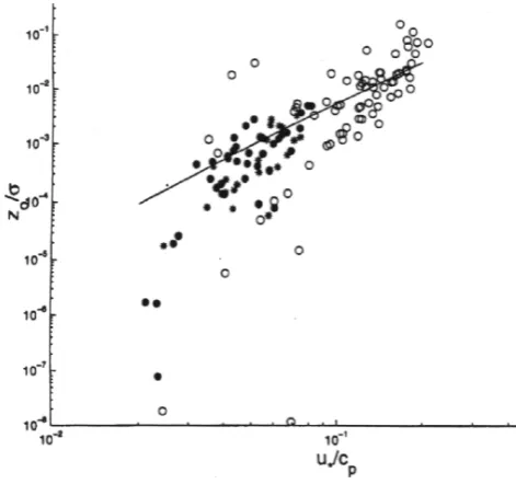
Fig. 5. Experimental dependence of normalized roughness,
Z0/ √
E, on the inverse wave age, U∗/Cp, following the paper
Drennan et al. (1999).
during the wave development. Such an increase is enclosed in the model due to the parameterization (12) of the dissipa-tion term. This is the essence of a physical treatment of the boundary layer parameters’ dependence on the sea state.
Further elaboration of the model is connected to a more detailed comparison of numerical and experimental depen-dencies, both for the effects named above and for the other, more fine effects, describing the boundary layer parameters’ dependence on the sea state. A total study of the model prop-erties will be done on the basis of test calculations for the most informative test problems presented, for example, in Efimov and Polnikov (1991) or The SWAMP group (1985).
V. G. Polnikov et al.: Numerical wind wave model with a dynamic boundary layer 371
References
Donelan, M. A.: Air-Water Exchange Processes (Physical Pro-cesses in Lakes and Oceans), Coastal and Estuarine Studies, 54, 19–36, 1998.
Drennan, W. M., Kahma, K. K., and Donelan, M. A.: On Momen-tum Flux and Velocity Spectra over Waves, Boundary-Layer Me-teorology, 92, 489–515, 1999.
Efimov, V. V. and Polnikov, V. G.: Numerical experiments on wind waves modeling, Oceanology, 25, 725–732, (English transla-tion), 1985.
Efimov, V. V. and Polnikov, V. G.: Numerical modeling of wind waves, Kyev. “Naukova dumka” Publishing House (in Russian), 1991.
Komen, G., Cavaleri, L., Janssen, P., et al.: Dynamics and Mod-elling of Ocean Waves, Cambridge University Press, 1994. Lavrenov, I. V.: Mathematical modeling of wind waves in a
spa-tially inhomogeneous ocean, St.- Petersburg. “Hydrometeoizdat” Publishing House, (in Russian), 1998.
Makin, V. K. and Kudryavtsev, V. N.: Coupled sea surface-atmosphere model, Pt.1 Wind over waves coupling, J. Geophys. Res., 104, 7613–7623, 1999.
Plant, W. J.: A relationship between wind stress and wave slope, J. Geophys. Res., 87, 1961–1967, 1982.
Polnikov V. G.: A third generation spectral model for wind waves, Izvestiya, Atm. and Ocean. Phys. 27, N8, (English transl.), 615– 623, 1991.
Polnikov V. G.: On a description of a wind-wave energy dissipa-tion funcdissipa-tion, Proc. Air-Sea Interface Symposium, ASI-94, Mar-seilles, France, 277–282, 1994.
Polnikov, V. G.: The study of nonlinear interactions in the wind wave spectrum, Dr. Sci. Thesis, Sebastopol, (in Russian), 1995. Polnikov, V. G.: A basing of the diffusion approximation derivation
for the four-wave kinetic integral and properties of the approxi-mation, Nonlin. Proc. Geophys., (this issue), 2002.
Snyder, R. L., Dobson, F. W., Elliott, J. A., and Long, R. B.: Array measurements of atmospheric pressure fluctuations above sur-face gravity waves, J. Fluid Mech., 102, 1–59, 1981.
The SWAMP group: Ocean wave modeling, New York and London, Plenum press, p. 256, 1985.
Zakharov, V. E and Pushkarev, A.: Diffusion Model of Interacting Gravity Waves on the Surface of Deep Fluid, Nonlin. Proc. Geo-phys., 6, 1–10, 1999.