www.clim-past.net/10/1453/2014/ doi:10.5194/cp-10-1453-2014
© Author(s) 2014. CC Attribution 3.0 License.
Evolution of the large-scale atmospheric circulation in response to
changing ice sheets over the last glacial cycle
M. Löfverström1,3, R. Caballero1,3, J. Nilsson1,3, and J. Kleman2,3 1Department of Meteorology, Stockholm University, Stockholm, Sweden
2Department of Physical Geography and Quaternary Geology, Stockholm University, Stockholm, Sweden 3Bolin Center for Climate Research, Stockholm University, Stockholm, Sweden
Correspondence to: M. Löfverström ([email protected])
Received: 10 March 2014 – Published in Clim. Past Discuss.: 4 April 2014 Revised: 22 June 2014 – Accepted: 24 June 2014 – Published: 31 July 2014
Abstract. We present modelling results of the atmospheric circulation at the cold periods of marine isotope stage 5b (MIS 5b), MIS 4 and the Last Glacial Maximum (LGM), as well as the interglacial. The palaeosimulations are forced by ice-sheet reconstructions consistent with geological evidence and by appropriate insolation and greenhouse gas concen-trations. The results suggest that the large-scale atmospheric winter circulation remained largely similar to the interglacial for a significant part of the glacial cycle. The proposed expla-nation is that the ice sheets were located in areas where their interaction with the mean flow is limited. However, the LGM Laurentide Ice Sheet induces a much larger planetary wave that leads to a zonalisation of the Atlantic jet. In summer, the ice-sheet topography dynamically induces warm temper-atures in Alaska and central Asia that inhibits the expansion of the ice sheets into these regions. The warm temperatures may also serve as an explanation for westward propagation of the Eurasian Ice Sheet from MIS 4 to the LGM.
1 Introduction
Over the last 2.6 million years (Gibbard and Kolfschoten, 2004) Earth’s climate has fluctuated between cold and warm periods – glacials and interglacials – characterised by the growth of major ice sheets over the Northern Hemi-sphere continents during cold periods and their retreat dur-ing warm periods. The most recent glacial cycle began some 115 000 years ago (115 kyr BP) following a relative mini-mum in the Northern Hemisphere summer insolation (Berger and Loutre, 2004). Reconstructions of ice-sheet development
through the subsequent 90 kyr (Peltier and Fairbanks, 2006; Stokes et al., 2012; Kleman et al., 2013) show global ice volume increasing in a step-wise fashion, with rapid growth bursts followed by longer periods of stagnation and cul-minating in the Last Glacial Maximum (LGM) spanning 19–23 kyr BP.
Initially, distinct ice sheets developed in the central Cana-dian Arctic, Quebec, Scandinavia and the Barents–Kara seas (Kleman et al., 2013), with possible smaller ice masses also in the Canadian Cordillera. An amalgamation process subsequently took place whereby these smaller and spa-tially separated ice sheets successively coalesced to finally form two massive and coherent ice sheets at the LGM, the Laurentide–Cordilleran ice sheet in North America and the Fennoscandian–Barents Sea ice sheet in Eurasia. At certain times, the mostly independent British–Irish Ice Sheet also formed part of the Eurasian Ice Sheet (Bradwell et al., 2008). The Laurentide was by far the larger of these LGM ice sheets, filling the northern part of North America from east to west and reaching southwards to approximately 42◦N.
(in conjunction with thermal forcing over the Gulf Stream re-gion, Kaspi and Schneider, 2011) induces northwesterly flow over central and eastern North America, yielding harsh win-ters there. The topographically driven wave is also largely responsible for the northeastward tilt of the Atlantic jet (Brayshaw et al., 2009), contributing to the milder winters of Europe compared with similar latitudes in North America (Seager et al., 2002).
Much effort has been devoted to understanding the cir-culation and climate of the LGM, including comprehen-sive proxy data syntheses (e.g. CLIMAP, 1981; MARGO, 2009, and QUEEN1), combined data–model reconstructions (Dail and Wunsch, 2014) and a large range of modelling studies, notably within the Paleoclimate Modelling Inter-comparison Projects2 (PMIP 1, 2, and 3) (Braconnot et al., 2007). Though there are appreciable model-to-model (Bra-connot et al., 2007; Li and Battisti, 2008; Otto-Bliesner et al., 2009; Kageyama et al., 2013a) and model–data discrepancies (Kageyama et al., 2006, 2013b; Otto-Bliesner et al., 2009), these studies generally depict an LGM climate substantially different from present. This is especially true in the Atlantic sector, which exhibits pronounced cooling of the northern North Atlantic Ocean, southward displacement of the sea-ice margin and southward-shifted, and, in some studies, a nearly zonally oriented atmospheric jet stream and storm track (e.g. Li and Battisti, 2008; Kageyama et al., 2013a; Ullman et al., 2014). A recent study by Ullman et al. (2014) attributed the massive mechanical forcing of the Laurentide Ice Sheet (in particular the ICE-5G reconstruction used in PMIP2; Peltier, 2004) as a key factor for the zonalisation of the jet. Simi-larly, in a model-based decomposition of various factors in-volved in creating the LGM climate, Pausata et al. (2011) ascribed the largest circulation change in the Atlantic region to the mechanical forcing of the Laurentide, rather than to increased albedo or reduced CO2.
The circulation during the long build-up phase to the LGM has received much less attention, despite the importance of this time-wise dominant period for understanding how the ocean, atmosphere and cryosphere reorganised as the world transitioned from an interglacial to a full-glacial state. To-day, it is well established that important terrestrial glaciation traces can only be understood in the context of glacial config-urations predating the LGM and of less than full-glacial size (Ljungner, 1949; Kleman, 1992; Fredin, 2002; Kleman et al., 2008). The significance of this long but less than full-glacial time period was recognised by Porter (1989), who coined the term “average glacial” conditions.
An important unanswered question about the pre-LGM climate is whether the atmospheric circulation characteris-tics were more similar to those in the LGM or in the inter-1Quaternary Environment of the Eurasian North, http://queen.
pangaea.de/
2http://pmip.lsce.ipsl.fr/, http://pmip2.lsce.ipsl.fr/, http://pmip3.
lsce.ipsl.fr/
glacial. Though smaller than they would eventually become at the LGM, the North American ice sheets nonetheless pre-sented a Rocky Mountains-sized topographic obstacle over eastern North America even in the early stages of the last glacial (Kleman et al., 2013). It is thus conceivable that they could have affected the circulation significantly, bringing it closer to the full LGM regime.
Another key issue is the extent to which atmospheric per-turbations induced by pre-LGM ice sheets helped shape the evolution of the ice sheets themselves (Beghin et al., 2014). Studies using idealised coupled atmosphere–ice-sheet mod-els focusing on the dynamics of a single continental-scale ice sheet on a flat continent (Roe and Lindzen, 2001; Li-akka et al., 2011; LiLi-akka, 2012) show that stationary wave– ice-sheet interaction can strongly influence both the spatial form and the temporal evolution of the ice sheet. Remote in-teractions between widely separated ice sheets mediated by stationary Rossby waves have received less attention (Lin-deman and Oerlemans, 1987; Kageyama and Valdes, 2000; Beghin et al., 2014). However there have been suggestions that the North American ice sheets excited a stationary wave train acting to warm northwestern Europe, suppressing ice growth there and potentially explaining why the Eurasian Ice Sheet was considerably smaller than the Laurentide in the latter stages of the glaciation (Roe and Lindzen, 2001). Sim-ilar questions arise regarding the documented absence of ma-jor ice sheets in places where they could be expected, such as Alaska and eastern central Siberia (Svendsen et al., 2004; Kleman et al., 2013), and the reasons for the general south-westward migration of the Eurasian Ice Sheet through the last glacial cycle (Sanberg and Oerlemans, 1983). Ice core analy-sis has revealed that the atmospheric dust concentration was considerably higher over the glacial cycle than in the present atmosphere (Mahowald et al., 1999). Theories have there-fore been put forth suggesting that dust deposition may have contributed to the absence of major ice sheets in Alaska and eastern central Siberia (Calov et al., 2005a, b; Krinner et al., 2006; Colleoni et al., 2009). Other studies show that changes in the the vegetation cover (Claussen et al., 2006; Colleoni et al., 2009) and SST (sea surface temperature) distributions (Colleoni et al., 2011) may also have contributed to hinder the development of ice sheets in these areas.
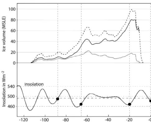
Figure 1. Evolution of the Northern Hemisphere ice volume and variations in daily average top of the atmosphere insolation during the northern summer solstice (60◦N) as a function of time. The solid and dotted lines in the top panel show the volume of the North American and Eurasian ice sheets, respectively and the dashed line is the total ice volume. The black dots in the lower panel mark the relative time of the simulations and the thick dashed line shows the mean insolation over the time period.
2 Model and experiments 2.1 Model
We employ the National Center for Atmospheric Research Community Atmospheric Model version 3 (CAM3) (Collins et al., 2004, 2006), using a spectral dynamical core with T85 (approximately 1.4◦) horizontal resolution and 26 hybrid
sigma-pressure levels in the vertical. Continental surfaces – including prescribed ice sheets – are represented by the Com-munity Land Model version 3 (CLM3) (Oleson et al., 2004). The ocean is represented by a motionless slab of fixed heat capacity, with ocean heat transport (OHT) represented by a prescribed climatological seasonally varying energy con-vergence field. The slab ocean also contains a thermody-namic sea-ice model. Further details on the prescription of the ice sheets and OHT are given below.
2.2 Ice sheets
Continental ice sheets over North America and Eurasia are prescribed from the recent reconstruction described by Kle-man et al. (2013), to which the reader is referred for full details. Briefly, the reconstruction spans the last glacial and employs a numerical ice-sheet model (specifically, the Uni-versity of Maine Ice Sheet Model (UMISM); Fastook and Chapman, 1989; Fastook, 1993) constrained by geological and geomorphological data. While reasonably reliable data
constraints for ice-sheet margins during pre-LGM times are available in some locations, other regions are less well con-strained, and there are no constraints at all on ice-sheet ele-vations and cross-sectional profiles. The strategy employed by Kleman et al. (2013) was to tune the ice-sheet model’s mass balance forcing using global model parameters to match well-constrained outline segments as closely as pos-sible where such constraints exist while relying on the model physics to capture ice-sheet elevations and outlines in un-constrained regions. This procedure bears some analogies to data assimilation, where a physically based model is used as an optimal extrapolator or predictor for regions or fields not directly constrained by data.
The resulting evolution of global ice volume is shown in Fig. 1, and is a good qualitative match to previous reconstruc-tions of global ice volume and inferences from sea-level data (Peltier and Fairbanks, 2006; Stokes et al., 2012). Snapshots of the spatial distribution of the ice sheets are shown in Fig. 2 and discussed further below.
UMISM outputs the net surface elevation, combining the topographic height with the ice thickness and isostatic de-pression of the bedrock due to ice loading, on a rectangu-lar grid with 100×100 points, covering from approximately 45◦N to the North Pole. This dataset is interpolated to T85 resolution and combined with the present day topography to create a palaeotopography with global coverage for use in the present simulations. We assume full glaciation of grid cells where the palaeodata is at least 250 m higher than the present day topography.
2.3 Ocean heat transport (OHT)
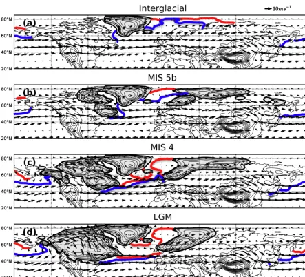
Figure 2. Evolution of the Northern Hemisphere topography over the glacial cycle (shading of ice sheets). The contour interval is 500 m and the outer contour line defines the edge of the ice sheets. The arrows show the wind vectors in winter along a model level (the nominal 800 hPa surface) and the blue (red) line the 50 % sea-ice margin in winter (summer).
between the two sets of simulations, but the overall qualita-tive conclusions of the study are robust to changes in OHT. 2.4 Experiments
As shown in Fig. 1, global ice volume during the last glacial grew in three main surges centred around∼110,∼70, and
∼25 kyr, while remaining roughly constant for extended pe-riods in between. To capture the main features of this evolu-tion, we focus on four time-slices representative of the main stages of the glacial cycle:
– Interglacial (Fig. 2a). This case represents conditions prior to inception of the last glacial and during mod-ern, pre-industrial conditions. It employs modern
topog-raphy and pre-industrial greenhouse gas concentrations and orbital parameters.
– MIS 4 (∼66 000 kyr BP; Fig. 2c). Approximately halfway into the glacial cycle, the ice volume in North America is now roughly twice as large as in Eurasia and consists of the two-domed proto-Laurentide Ice Sheet and a number of smaller freestanding ice sheets in the Cordilleran region. The Keewatin Dome covers most of the Canadian archipelago and northern central parts of the Canadian mainland. In the north, a small gap to the Rocky Mountains still exists, widening to approxi-mately 1000 km further south. On the northeastern and southeastern fringes, towards Baffin Bay and the North Atlantic, ice everywhere reaches the sea. The Quebec Dome is the larger of the two (the figure suggests the op-posite but that is due to the map projection) and extend almost as far south as 42◦N over the eastern continent. The Eurasian Ice Sheet is here at its maximum zonal ex-tent. Both the Eurasian and proto-Laurentide ice sheets are in this case about 2500 m high.
– LGM (MIS 2, ∼20 000 kyr BP; Fig. 2d). Under full glacial conditions, the Laurentide Ice Sheet is a single-domed continent-wide entity that dwarfs the Rockies. The centre of mass is in the middle of the continent, as in the ICE-5G reconstruction (Peltier, 2004) used in PMIP2. Our reconstruction of the Laurentide ice dome is lower, however, about 3500 m as compared to about 4500 m in ICE-5G. In Eurasia the ice margin has re-treated in the east and shifted the centre of mass to Scan-dinavia, but achieves its greatest meridional extent and even covers most of the British Isles. The total ice vol-ume in the Northern Hemisphere corresponds to about 100 m of sea-level equivalent, of which the Laurentide and Eurasian ice sheets make up roughly 80 and 20 %, respectively. These numbers agree well with the PMIP3 ice-sheet reconstructions.
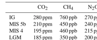
For each glacial simulation, we set the orbital clock to the nominal time of the ice-sheet reconstruction. We also adjust the concentrations of long-lived greenhouse gases to typical values estimated from the EPICA (European Project for Ice Coring in Antarctica) Dome C ice core (Petit et al., 1999; Spahni et al., 2005); see Table 1. These values are rounded off to the nearest 5 ppmv (parts per million by volume) for CO2 and 5 ppbv (parts per billion by volume) for CH4and N2O. The concentrations of chlorofluorocarbons (CFC11and CFC12) are identically zero in all simulations and we use the pre-industrial aerosol distribution. All simulations use mod-ern pre-industrial vegetation cover adjusted by the glacier mask.
To test the sensitivity of the results to orbital parameters and greenhouse gas concentrations, we conduct an additional set of simulations in which topography is held fixed at its interglacial distribution while orbital parameters and green-house gases take on glacial values. For the MIS 4 case we also run two additional simulations where the Eurasian and North American ice sheets are removed in turn to further
in-Table 1. Concentrations of long-lived greenhouse gases in the dif-ferent simulations. All instances are given per volume.
CO2 CH4 N2O
IG 280 ppm 760 ppb 270 ppb MIS 5b 210 ppm 450 ppb 240 ppb MIS 4 195 ppm 460 ppb 215 ppb LGM 185 ppm 350 ppb 200 ppb
vestigate their relative influence on the atmospheric flow pat-terns. A list of the various combinations of boundary condi-tions used in this study is shown in Table 2. Results presented below are based on seasonal averages over 30 years after the simulated climates have reached statistical equilibrium. The spin-up of the model takes about 20–30 model years and the climate is assumed to have equilibrated when the long-term trends in the global- and annual-mean surface temperature and sea-ice concentration become negligible.
3 Results
This section presents the main results from the simulations of the four time slices discussed above. For brevity we present only results from the interglacial and MIS 5b simulations with interglacial OHT and MIS 4 and LGM simulation with LGM OHT; as noted in Sect. 2.3, changing OHT does not affect our qualitative conclusions. The full set of simulation results, showing the sensitivity to OHT, is presented in the Supplement.
3.1 Surface temperature
As shown in Table 3, global-mean surface temperatures con-tinuously decrease across the simulations, dropping by about 5◦C from the interglacial to the LGM irrespective of sea-son. To put this number in perspective with the rest of the modelling community, Braconnot et al. (2007) and Otto-Bliesner et al. (2009) found that the annual global-mean sur-face temperature in the fully coupled PMIP2 models is be-tween 3.1 and 5.8◦C colder at the LGM compared to the interglacial, where the number for CCSM3 (Community Cli-mate System Model version 3), which uses the same atmo-spheric component as in this study, is 4.5◦C (Otto-Bliesner
et al., 2006, 2009). More recent generations of models with updated boundary conditions report values between 4.5 and 5.5◦C (see, e.g. Brady et al., 2013; Kageyama et al., 2013a; Ullman et al., 2014).
Table 2. Configuration of boundary conditions used in the study (marked by×). The oceanic heat fluxes for interglacial and LGM conditions are denoted byQIGandQLGMand the interglacial and reconstructed palaeotopography by8IGand8Palaeo, respectively. The sensitivity tests of the palaeotopography with only the North American or Eurasian ice sheets present are denoted by8NAand8EA.
QIG QLGM
8IG 8Palaeo 8NA 8EA 8IG 8Palaeo 8NA 8EA
IG × – – – × – – –
MIS 5b × × – – × × – –
MIS 4 × × × × × × × ×
LGM × × – – × × – –
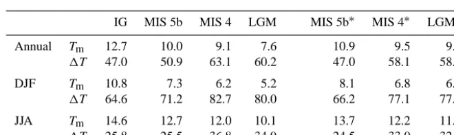
Table 3. Global-mean surface temperatureTm(◦C) and Northern Hemisphere Equator–pole (average from 0–10 to 80–90◦N) temperature difference1T (◦C) for the four time slices. Asterisks indicate sensitivity simulations employing interglacial topography.
IG MIS 5b MIS 4 LGM MIS 5b∗ MIS 4∗ LGM∗
Annual Tm 12.7 10.0 9.1 7.6 10.9 9.5 9.3
1T 47.0 50.9 63.1 60.2 47.0 58.1 58.2
DJF Tm 10.8 7.3 6.2 5.2 8.1 6.8 6.9
1T 64.6 71.2 82.7 80.0 66.2 77.1 77.8
JJA Tm 14.6 12.7 12.0 10.1 13.7 12.2 11.6
1T 25.8 25.5 36.8 34.9 24.5 33.0 32.9
heat flux convergence) is 7.9◦C. The corresponding number
for IPSL_CM5 with PMIP3 boundary conditions is 7.7◦C (Kageyama et al., 2013a). The values for the pre-industrial and LGM presented in Table 3 are thus well within the un-certainty range of the PMIP models.
In the sensitivity simulations in which the ice sheets are eliminated (indicated by asterisks in the table), the tempera-ture drop is only about 3.4◦C; this implies that the ice sheets themselves account for about one-third of the global temper-ature decrease from interglacial to LGM. This differs from the situation in Antarctica, where sensitivity studies with the same model used here show no appreciable temperature change when the Antarctic ice sheet is eliminated (Goldner et al., 2013).
The mean Northern Hemisphere Equator–pole tempera-ture gradient generally increases as temperatempera-tures cool, in line with expectations of polar-amplified cooling (Singarayer and Valdes, 2010), though interestingly the LGM has a slightly smaller gradient than MIS 4. The gradient grows by approx-imately 25 % from the interglacial to the LGM in winter and almost 40 % in summer; this leads to substantial strength-ening of the midlatitude westerlies with important conse-quences for the response to topography, as discussed below.
The somewhat larger meridional temperature gradient in MIS 4 compared to the LGM is related to the difference in Earth’s orbital parameters at the nominal time of the simu-lations. The Northern Hemisphere high latitudes in MIS 4 receive more insolation in spring compared to the LGM but
the summer and fall insolation is less (not shown), thus ren-dering the Arctic generally colder over a large part of the year. When introducing the ice sheets this effect is intensi-fied as their high albedo helps to cool regions with a seasonal snow cover in the sensitivity simulations. The annual insola-tion in the tropics is also slightly higher in MIS 4 compared to the LGM, which acts to further strengthen the meridional temperature gradient.
3.2 Evolution of the winter circulation
0° 20°N 40°N 60°N 80°N
(a)
0° 20°N 40°N 60°N 80°N
Reanalysis
−500 −400 −300 −200 −100 0 100 200 300 400 500
0° 20°N 40°N 60°N 80°N
(b)
0° 20°N 40°N 60°N 80°N
Interglacial
−500 −400 −300 −200 −100 0 100 200 300 400 500
0° 20°N 40°N 60°N 80°N
(c)
0° 20°N 40°N 60°N 80°N
MIS 5b
−500 −400 −300 −200 −100 0 100 200 300 400 500
0° 20°N 40°N 60°N 80°N
(d)
0° 20°N 40°N 60°N 80°N
MIS 4
−500 −400 −300 −200 −100 0 100 200 300 400 500
0° 20°N 40°N 60°N 80°N
(e)
0° 20°N 40°N 60°N 80°N
180° 135°W 90°W 45°W 0° 45°E 90°E 135°E 180°
180° 180°
LGM
−500 −400 −300 −200 −100 0 100 200 300 400 500
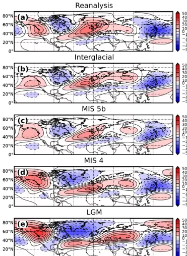
Figure 3. The 300 hPa eddy geopotential field averaged over the winter months (DJF). The contour interval is 50 m. Note the zonalisation of the geopotential height gradient over the Atlantic Ocean in the LGM simulation.
meridionally tilted precipitation field (see, e.g. Hoskins and Valdes, 1990; Lee, 2000; Chang et al., 2002; Held et al., 2002; Vallis and Gerber, 2008; Brayshaw et al., 2009, 2011, for discussions on the existence of stormtracks and how they are influenced by various forcing agents).
The results from the glacial simulations suggest that the interglacial disposition of the stationary waves and zonal jet was maintained for a significant portion of the glacial cycle,
0° 20°N 40°N 60°N 80°N
(a)
0° 20°N 40°N 60°N 80°N 0° 20°N 40°N 60°N 80°N 0° 20°N 40°N 60°N 80°NReanalysis
1 2 3 4 5 6 7 8 0° 20°N 40°N 60°N 80°N(b)
0° 20°N 40°N 60°N 80°N 0° 20°N 40°N 60°N 80°N 0° 20°N 40°N 60°N 80°NInterglacial
1 2 3 4 5 6 7 8 0° 20°N 40°N 60°N 80°N(c)
0° 20°N 40°N 60°N 80°N 0° 20°N 40°N 60°N 80°N 0° 20°N 40°N 60°N 80°NMIS 5b
1 2 3 4 5 6 7 8 0° 20°N 40°N 60°N 80°N(d)
0° 20°N 40°N 60°N 80°N 0° 20°N 40°N 60°N 80°N 0° 20°N 40°N 60°N 80°NMIS 4
1 2 3 4 5 6 7 8 0° 20°N 40°N 60°N 80°N(e)
0° 20°N 40°N 60°N 80°N 0° 20°N 40°N 60°N 80°N 0° 20°N 40°N 60°N 80°N180° 135°W 90°W 45°W 0° 45°E 90°E 135°E 180°
180° 180°
LGM
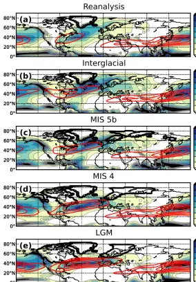
1 2 3 4 5 6 7 8Figure 4. Evolution of the winter (DJF) precipitation (mm day−1) over the glacial cycle. The ice sheets are indicated by the heavy black contours and the red contour lines show the 300 hPa zonal wind speed (10 m s−1contours starting at 30 m s−1).
downstream of the fully developed Laurentide Ice Sheet is deep and zonally extensive, yielding a strong and essentially zonal jet. A similar result was obtained by Li and Battisti (2008); Kageyama et al. (2013a); Ullman et al. (2014) using fully coupled models with LGM boundary conditions fol-lowing the PMIP2 protocol. However, simulations with the updated PMIP3 boundary conditions yield a slightly more tilted Atlantic jet (e.g. Kageyama et al., 2013a; Ullman et al., 2014).
The sea-ice margin (Fig. 2) moves equatorward in both ocean basins as the glacial progresses. However, the North Atlantic remains largely ice-free through MIS 5b, and even in MIS 4 the ice margin has a clear northeastward tilt parallel to the prevailing winds, presumably because warm advection by the winds prevents sea-ice formation off western Europe. It
is only at the LGM, when the winds become perfectly zonal, that the ice line reaches south to Iberia.
expand the zonalised region but it is primarily the high LGM ice-sheet topography that causes the shift of the jet axis.
The sea-ice cover obtained in our LGM simulation resem-bles the CLIMAP (1981) reconstruction which is more ex-tensive than in more recent proxy-data reconstructions, es-pecially in the eastern Atlantic where the perennial sea-ice line is found to not venture past 55◦N (Kucera et al., 2005; De Vernal et al., 2005, 2006; MARGO, 2009). Recent mod-elling studies also show a more moderate Atlantic sea-ice cover than obtained here; see, e.g. Braconnot et al. (2007); Li and Battisti (2008); Pausata et al. (2011). The reason for the very extensive Atlantic sea-ice cover obtained in this study is that our OHT is based on the second LGM equilib-rium state discussed by Brandefelt and Otto-Bliesner (2009), which is believed to be close to the model’s true steady state. In this state the Atlantic Meridional Overturning Circulation (AMOC) is strongly reduced and sea-ice is therefore able to form over a larger area of the ocean (cf. Fig. 2 in Brandefelt and Otto-Bliesner (2009)).
Consistent with the discussion above, the storm track un-dergoes a similar transition as the jet stream and retains much of its meridional tilt in MIS 5b and MIS 4 (Fig. 4). At the LGM, however, it becomes almost completely zonalised over the Atlantic Ocean.
The LGM storm track is also more meridionally confined and the precipitation does not reach as far inland over Eurasia as in the previous cases, likely because the simulated more extensive sea-ice cover in the North Atlantic limits evapora-tion and yields drier air masses moving into Europe. Neither case shows a significant amount of winter precipitation on the ice sheets themselves. There is some precipitation falling on the southwestern and western edges but almost nothing in the interior. In Eurasia this is due to the ice sheets’ northerly location, where the bulk of the precipitation falls south of the main ice sheet. The North American continent is shielded from the Pacific cyclones by the Rockies, making the air in the interior of the continent relatively dry and less prone to precipitate. We will see later that the picture is different in the summer season.
We can make use of the low-level winds in Fig. 2 to give a rationale for the evolution of the planetary waves. The to-pography of the Rockies yields an upstream ridge over the eastern Pacific as part of the Rossby wave response, adding anticyclonic curvature of the mean flow: as the air flows onto the topography the effective column depth decreases and the mean flow deflects southwards to conserve potential vortic-ity. On the eastern side of the mountain range the situation is the opposite and the mean flow follows a cyclonic path as a response to the increasing fluid depth (see Appendix A for a discussion on potential vorticity conservation). A con-sequence of the meridional deflection of the mean flow is that the strongest low-level winds are channelled between the Rockies and the incipient Laurentide Ice Sheet, with little flow normal to the ice-sheet topography. Consequently, the mechanical stationary wave forcing by the ice sheet is small,
and the outline of the planetary waves remains largely similar to the present day.
This explanation is applicable to MIS 5b and partly also to MIS 4, as the lowland corridor in the interior of the North American continent is present in both cases. However, in the latter case the westward expansion of the Keewatin Dome in northern Canada partially pinches off the channel, forcing flow over the ice sheet in the north. Further south, the flow crosses the Rockies in a similar fashion as in the interglacial, but overall there is a more substantial interaction between the ice sheets and the mean flow which is reflected in an am-plified planetary wave response and an eastward shift of the lee-side trough from the Hudson Bay to the Labrador Sea.
The topographic profile of the LGM Laurentide Ice Sheet is structurally very different from the earlier stages of the glacial cycle. The ice volume is nearly twice as large as at MIS 4 (Fig. 1), and the lowland region east of the Rockies is entirely filled up and instead constitutes the highest part of the continent. Consequently, the topographic influence is much more substantial than earlier, and the low-level wind field over the eastern Pacific (Fig. 2d) is subject to an even stronger meridional splitting. In fact, the entire flow normal to the ice sheet is obstructed and forced on a poleward track. A similar meridional splitting was also found by Manabe and Broccoli (1985) and Cook and Held (1988). Note that the anticyclone over the northeastern Pacific is strong enough to even force low-level easterlies over parts of Alaska and Siberia. This is also hinted in Fig. 3e where the upper tropo-spheric anticyclone is significantly stronger than earlier and protrudes far into eastern Siberia.
The Eurasian Ice Sheet topography is located too far to the north to be able to interact with the strong midlatitude zonal-mean flow and thereby influence the stationary wave field. In both MIS 5b and MIS 4 the strongest westerly winds are found over central Europe, whereas the southern ice mar-gin is located over Scandinavia. Even though the ice sheet expands equatorward when moving into the LGM, the zon-alisation of the Atlantic storm track shifts the westerly winds southwards and the flow-topography interaction therefore re-mains small.
3.3 Evolution of the summer circulation
0° 20°N 40°N 60°N 80°N (a)
0° 20°N 40°N 60°N 80°N
Reanalysis
−250 −200 −150 −100 −50 0 50 100 150 200 250
0° 20°N 40°N 60°N 80°N (b)
0° 20°N 40°N 60°N 80°N
Interglacial
−250 −200 −150 −100 −50 0 50 100 150 200 250
0° 20°N 40°N 60°N 80°N (c)
0° 20°N 40°N 60°N 80°N
MIS 5b
−250 −200 −150 −100 −50 0 50 100 150 200 250
0° 20°N 40°N 60°N 80°N (d)
0° 20°N 40°N 60°N 80°N
MIS 4
−250 −200 −150 −100 −50 0 50 100 150 200 250
0° 20°N 40°N 60°N 80°N (e)
0° 20°N 40°N 60°N 80°N
180° 135°W 90°W 45°W 0° 45°E 90°E 135°E 180°
180° 180°
LGM
−250 −200 −150 −100 −50 0 50 100 150 200 250
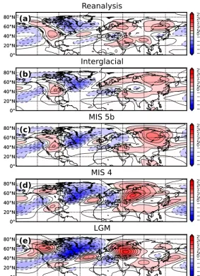
Figure 5. Evolution of the 300 hPa eddy geopotential in the summer (JJA) season. The contour interval is 25 m.
Ting (1994) for comprehensive discussions on the summer stationary waves.
Figure 5 shows the upper tropospheric eddy geopotential averaged over the summer months. One can readily see a pro-gressive development of the wave field over the course of the glacial cycle. Already at MIS 5b there is some amplifica-tion of the height anomalies over the northern parts of North America and one can also see an additional wave train prop-agating over the Atlantic Ocean into Europe. The response does resemble the linear topographic wave, or low mountain wave, discussed by, e.g. Valdes and Hoskins (1991), Cook and Held (1992), and Ringler and Cook (1997). The am-plitude of these waves is clearly linked to the size of the ice topography as they are reinforced but stay in approxi-mately the same location when the ice sheets grow larger. The anticyclone associated with the divergent flow in the up-per troposphere over the North American continent is grad-ually being weakened and shifted southward as the glacial
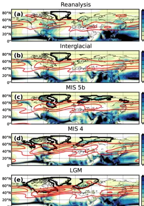
Figure 6. Evolution of the winter (JJA) precipitation (mm day−1) over the glacial cycle. The ice sheets are indicated by the heavy black contours and the red contour lines show the 300 hPa zonal wind speed (10 m s−1contours starting at 10 m s−1).
diabatic cooling (Ringler and Cook, 1999; Liakka, 2012). To better understand the influence of the ice sheets on the plane-tary waves the reader is referred to the supplemenplane-tary mate-rial where we show the development of the eddy geopotential field both for the fully forced cases as well as the sensitivity experiments with eliminated ice sheets.
Figure 6 shows the spatial distribution of the summer precipitation. The tropics dominate the picture but one can clearly see that the midlatitude storm tracks are weaker and less organised than in winter and the precipitation is there-fore dispersed over a larger area. The warm air transports water vapour far inland and precipitates over the ice sheets. One can also see a precipitation maximum on the windward side of the ice sheets that encourages their westward expan-sion in time. There is also an additional maximum along the southern edge of the Eurasian Ice Sheet that is a
re-sult of the anticyclonic circulation in Fig. 5. Likewise, the drier conditions east of the Eurasian Ice Sheet at the LGM comes from advection of cold air in the southward branch of the circulation cell.
0° 20°N 40°N 60°N 80°N (a) 0° 20°N 40°N 60°N 80°N MIS 5b −9 −6 −3 0 3 6 9 0° 20°N 40°N 60°N 80°N (c) 0° 20°N 40°N 60°N 80°N MIS 4 −9 −6 −3 0 3 6 9 0° 20°N 40°N 60°N 80°N (e) 0° 20°N 40°N 60°N 80°N
180° 135°W 90°W 45°W 0° 45°E 90°E 135°E 180°
180° 180° LGM −9 −6 −3 0 3 6 9 (b) MIS 5b −30 −20 −10 0 10 20 30 (d) MIS 4 −30 −20 −10 0 10 20 30 (f)
180° 135°W 90°W 45°W 0° 45°E 90°E 135°E 180°
180° 180° LGM −30 −20 −10 0 10 20 30
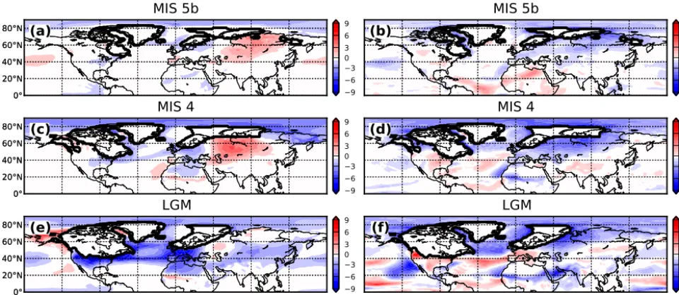
Figure 7. The panels on the left show the difference in average summer (JJA) surface temperature (K) between the full glacial simulations and the no-ice-sheet simulations; see details in the text. The panels on the right show the corresponding difference in the total cloudiness (%). Note that values over the ice sheets are masked out for display purposes.
surface albedo – change between the no-ice-sheet and glacial simulations. We make no attempt to decompose this further.
Results from the sensitivity experiments are shown in Fig. 7. It is apparent that the presence of the ice sheets has a large influence on both the regional temperature and cloud cover. The Atlantic sector features a progressively expand-ing area of coolexpand-ing while there are relatively warm anoma-lies in Alaska and central Asia (note that similar results are obtained regardless of the OHT; see supplementary mate-rial). A similar warm anomaly southeast of the Eurasian Ice Sheet has been found in previous studies of the LGM; see e.g. Manabe and Broccoli (1985), Rind (1987), Felzer et al. (1996), Feltzer et al. (1998), and Abe-Ouchi et al. (2007). Warmer temperatures in Alaska were also reported by e.g. Otto-Bliesner et al. (2006) and Abe-Ouchi et al. (2007), where the latter compared the LGM and interglacial temper-atures from several different models.
The increasingly dominant anticyclonic circulation over Alaska and Siberia implies subsiding motion there and there-fore generally reduced cloudiness as seen in Fig. 7. The land surface thus absorbs a larger amount of downwelling short-wave radiation, which leads to warmer temperatures. The an-ticyclonic circulation also implies warm air advection into the target areas that helps to increase the temperatures even further.
The strongly diminished temperature anomaly in Eurasia in the LGM simulation (Fig. 7e) is somewhat at odds with this picture, however, since the anticyclone is at its strongest. This weakening of the warm anomaly is likely the result of cold westerly temperature advection from the Atlantic (which remains ice-covered through the summer; Fig. 2d) and counteracts the radiative heating in Siberia. This does
not happen to the same extent in MIS 4 as the anticyclone is located farther to the east and the temperatures in Europe are not as low as at the LGM.
The colder surface temperature in the Atlantic region is a result of the extensive sea-ice cover. Figure 2 shows that in winter, the North American ice sheets force strong northerly winds that advect cold polar air over the eastern parts of the continent and also the western Atlantic. The cold air advec-tion thus helps to shift the sea-ice line farther equatorward than it would if the ice sheet was not present. In the warm season the extensive sea-ice limits the evaporation over the northern North Atlantic and results in a net reduction of the cloudiness as seen in the right column in Fig. 7. A reduced cloudiness implies more down-welling of shortwave radia-tion but the melting process of snow and sea-ice is slow and inefficient due to the high surface albedo. The colder air over the ocean is also advected by the westerly winds (Fig. 2) to Europe where it holds down the surface temperature and helps sustain and build the western part of the Eurasian Ice Sheet over the warm season (note that similar temperature anomalies are obtained regardless of the OHT, see supple-mentary figures). Note that the LGM simulation features an area of increased cloudiness south of the sea-ice margin that is not reflected in the precipitation pattern. A decomposition (not shown) reveals that this is related to a larger fraction of low-level clouds. We make no attempt to evaluate the pro-cesses involved in generating this signal.
0° 20°N 40°N 60°N 80°N (a)
0° 20°N 40°N 60°N 80°N
−9 −6 −3 0 3 6 9
0° 20°N 40°N 60°N 80°N (b)
0° 20°N 40°N 60°N 80°N
180° 135°W 90°W 45°W 0° 45°E 90°E 135°E 180°
180° 180° −9
−6 −3 0 3 6 9
Figure 8. Same as in Fig. 7c for the MIS 4 Laurentide Ice Sheet to-pography in the upper panel and the Eurasian Ice Sheet toto-pography in the lower panel.
in Fig. 8. It is obvious that most of the temperature response in the western hemisphere and Europe is linked to the pres-ence of the Laurentide Ice Sheet, whereas the relative tem-perature anomaly in Asia is a result of the circulation change induced by the Eurasian Ice Sheet.
4 Discussion
4.1 Winter stationary waves
The results presented in Figs. 3 and 4 show some very sub-stantial changes in the winter stationary waves, Atlantic jet stream and storm tracks between the interglacial and LGM. These changes do not come about as a smooth progression through time, however. Our MIS 5b simulation, which is rep-resentative of the first 30–40 kyr of the glacial (see Fig. 1), shows a circulation essentially unchanged from the inter-glacial, despite the considerable ice sheets developing in eastern North America and Eurasia. Stationary wave ampli-tudes increase during the subsequent 30–40 kyr, represented by our MIS 4 simulation, and the jet strengthens consider-ably, but the overall structure of the stationary waves remains very similar to that in the interglacial – retaining, in particu-lar, the characteristic southwesterly tilt of the Atlantic jet. It is arguably only in the LGM simulation, representing some 5–10 kyr around the peak of the last glacial, that qualitative changes can be seen, with a full zonalisation of the jet and a perceptible shift towards more zonally elongated stationary wave structures: note that throughout the interglacial, MIS 5b and MIS 4 simulations there are three peaks and troughs in the eddy height field along latitude lines in the midlatitudes (Fig. 3b–d), while there are clearly only two in the LGM sim-ulation.
The shift toward longer stationary waves is consistent with the predictions of simple linear barotropic theory (see Ap-pendix A). A key result of the theory is that the stationary wave number Ks=
√
β/[u], where [u] is the zonal-mean zonal wind and β is the meridional gradient of the
Corio-−400 −2000 200 400
(a)
Interglacial
0 90◦E 180◦ 90◦W 0
0 1 km 2 km 3 km
(c)
(b)
LGM
0 90◦E 180◦ 90◦W 0
(d)
5 10 15 20 25 30 [u]
0 200 400 600 800
σ
(e) (e)
1 2 3 4 5
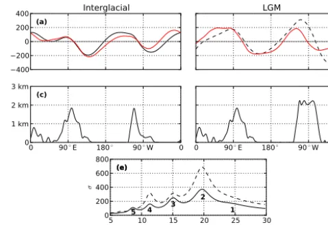
Figure 9. The top panels (a, b) show a comparison of the midtro-pospheric eddy geopotential (m) at 45◦N computed by the linear barotropic model (black) and the atmospheric circulation model (red) at 500 hPa. The panels on the left show the interglacial and the panels on the right the fields from the LGM simulations. The corresponding topographic profiles are shown in the middle pan-els (c, d). In the lower panel (e) we show the standard deviation
of the geopotential height response(σ=
q
[ψ02])as a function of the zonal mean wind[u]. Here we use a more generous damping timescale ofr−1=20 days for display purposes. One can clearly see how different wave numbers resonate at certain wind speeds. The solid line uses the present day topography (c) and the dashed line the LGM topography (d).
lis parameter. As discussed in Sect. 3.1, the Equator-to-pole temperature gradient increases as the LGM is approached resulting in stronger winds (the zonal-mean wind averaged between 800 and 150 hPa increases by about 30 % from 18 m s−1 in the interglacial to 24 m s−1 in the LGM simu-lation) and thus smallerKs, or longer stationary waves. In addition, the zonal width of the North American orography – which forces the stationary wave train over the Atlantic – in-creases very substantially from the interglacial to the LGM, so that the forcing of the stationary waves also shifts towards longer scales.
replicated also in other models as long as they faithfully re-produce the large-scale flow over the Rockies.
A similar effect occurs for the Eurasian Ice Sheet, which also fails to excite stationary waves in the early stages of the glacial. In this case, warm southwesterly advection by the Atlantic jet presumably limits the southward extension of the Fennoscandian Ice Sheet, automatically confining this ice sheet to a region of weak climatological westerlies which are unable to excite large stationary waves.
Although the simple linear model captures the main fea-tures of the LGM stationary waves with surprising quantita-tive accuracy, this is likely a fortuitous result from the choice of parameter values and in particular of the model’s chan-nel geometry (Held, 1983). GCM simulations by Cook and Held (1992) show that substantial deviations from linearity are possible as topographic height increases, and these devi-ations are complex and model-dependent (Held et al., 2002). In fact, model intercomparison exercises show a wide range of responses by different models all driven by the same LGM topography (Li and Battisti, 2008); among these, the model used here (CAM3) has a larger-than-average response, with most other models showing an LGM circulation that departs less dramatically from the interglacial (but note that Li and Battisti, 2008, found good agreement between their LGM re-sults using CAM3 and available proxy data). Overall, the conclusion that can be drawn from this discussion is that the atmospheric circulation’s response to the Northern Hemi-sphere ice sheets during winter may have been muted through large parts of the last glacial cycle, and possibly even at the LGM.
4.2 Self-induced temperature anomalies in summer A key factor controlling the evolution of the ice sheets is the summer surface temperature, as it is in the warm sea-son that significant ablation occurs. The temperature at the top of the ice sheets is generally below freezing and the sum-mer ablation is therefore restricted to the marginal ablation zones at lower elevation. Figure 7 shows that the presence of the ice sheets induces warm surface temperature anoma-lies in Alaska and Siberia. A similar temperature response has been obtained in previous modelling studies of the sen-sitivity to the LGM ice sheets; e.g. in Manabe and Broccoli (1985), Rind (1987), Felzer et al. (1996), Feltzer et al. (1998), Abe-Ouchi et al. (2007), and Otto-Bliesner et al. (2006). That the model simulates warmer temperatures in these particular regions is intriguing, as we know from geological evidence that Alaska was left largely ice-free over the entire glacial cy-cle (Clague, 1989). At the same time, the Eurasian ice com-plex was limited to the northernmost parts of the continent and its centre of mass shifted southwestwards as the glacial proceeded (Svendsen et al., 2004; Kleman et al., 2013). In the simulations the summer surface temperature in Alaska stays approximately the same as in the interglacial climate throughout the entire glacial cycle (the pollen-based
temper-ature reconstruction of the LGM by Bartlein et al., 2011, suggests that the surface conditions in Alaska were indeed comparable, if not even slightly warmer than in the present climate) and the region south of the Eurasian Ice Sheet at MIS 4 is even slightly warmer than in the interglacial simu-lation (not shown). It is thus conceivable that the self-induced warm anomaly in central Siberia may have contributed to limit the glaciation in this region, possibly in conjunction with albedo effects from dust deposition (Mahowald et al., 1999; Calov et al., 2005a, b; Krinner et al., 2006; Colleoni et al., 2009) and the vegetation cover (Claussen et al., 2006; Colleoni et al., 2009). This warm anomaly may also help to explain the westward shift of the ice sheet when moving from MIS 4 to the LGM together with the upslope precipitation in the west as discussed by Sanberg and Oerlemans (1983).
5 Conclusions
We summarise our conclusions as follows:
– During winter, the pexisting stationary wave re-sponse to the Rocky Mountains limits the flow’s inter-action with the ice sheets during MIS 5b and 4, and the influence of these ice sheets on the tropospheric circu-lation is therefore surprisingly small despite their very substantial size.
– During MIS 5b and 4, the general outline of the winter stationary waves is largely unchanged from the inter-glacial and the jet axis in the Atlantic sector retains the characteristic southwest–northeast tilt.
– Only when the Laurentide Ice Sheet is fully developed are the planetary waves strongly influenced and the At-lantic jet axis is zonalised as a result. A highly simpli-fied linear stationary wave model suggests that the in-creased mean wind speed during the LGM is the key parameter controlling the structural changes in the cir-culation.
– In the summer season, on the contrary, the ice sheets strongly influence the eddy geopotential field and an anticyclonic circulation develops in Alaska and cen-tral Asia as a result. Anticyclonic circulation implies less cloudiness and more shortwave radiation can there-fore reach the surface. It is thus plausible that Alaska and central Asia were left largely ice-free due to self-induced warm anomalies at the surface.
Eurasian Ice Sheet, but may have contributed slightly to the westward shift of the ice-sheet-mass centre. – Based on the results presented in this study we propose
Appendix A:
A1 Notes on linear stationary wave theory
We here present some background on linear stationary wave theory that is helpful for the interpretation of the simu-lated atmospheric flows. The potential vorticity is a con-served3property for all fluid elements that essentially mea-sures the ratio between the absolute vorticity and the effec-tive fluid depth. Rossby (1940) showed that for a non-viscous barotropic fluid this can be expressed as
D Dt
f+ζ
H
=0, (A1)
where D/Dt=(∂/∂t+v·∇)is the material derivative,v=
(u, v)is a vector containing the zonal and meridional compo-nents of the wind field and∇=(∂/∂x, ∂/∂y)is the horizon-tal gradient operator. The numerator is here the sum of the planetary (f) and relative vorticity (ζ ≡kˆ·∇×v, wherekˆ is the unit vector in the radial direction) and H is the fluid depth. Equation (A1) says that if the fluid depth change, e.g. by a topographic obstacle, the absolute vorticity has to change in the same direction to conserve their internal ratio.
Assuming a low amplitude topographic forcing (hTH) and linearising around a time-independent quasi-geostrophic zonal mean flow (u= [u] +u∗,v=v∗wherev∗∼u∗ [u], here [·] and (∗) denotes zonal mean and zonal perturba-tion quantities, respectively) at a midlatitude β plane (f =
f0+βy), we can define the perturbation velocity field from a geostrophic stream function as(u∗, v∗)=kˆ×∇ψ∗and thus ζ∗= ∇2ψ∗. The resulting equation has wave solutions of the form(ψ∗, hT)=Re(ψ0, h0)expi(kx+ly)and the complex amplitude of the height anomaly is
ψ0=f0
H
h0 K2−K2
s −iR
, (A2)
whereK= √
k2+l2is the total wave number and the sta-tionary wave number is defined as
Ks= s
β
[u]. (A3)
We have also added a linear damping (R=rK2/ k[u]) to en-sure bounded solutions as Eq. (A2) resonates for a total wave number equal to the stationary wave number. A stronger wind implies a smaller wave number and thus longer station-ary waves. The amplitude of the waves, however, is propor-tional to the magnitude of the topography. This highly sim-plified linear model thus suggests that the structural changes in the stationary wave field at the LGM is a result of the in-creased mean wind speed as it projects onto a smaller sta-tionary wave number. The massive changes in the surface to-pography merely give more weight to the resonant wave.
3Note that true conservation of potential vorticity is only
possi-ble for idealised frictionless and strictly adiabatic fluids.
To quantify this premise we compute the standard devia-tion of the wave soludevia-tion in Eq. (A2)(σ=
q
[ψ02])as a func-tion of the zonal mean wind speed when using the interglacial and LGM topographic profiles at midlatitudes (Fig. 9c, d). We apply the original model settings used by Charney and Eliassen (1949):f0=f (45◦N);H=8 km; and a meridional wave number with the half-wavelength of 35◦in latitude but a weaker damping, andr−1=20 days, to make the resonant peaks more distinct. These results are presented in Fig. 9e, clearly showing how the model resonates for lower station-ary wave numbers as the wind speed increases. It is apparent that the larger topography at the LGM primarily influence the amplitude of the stationary waves. For wind speeds of approximately 20 m s−1, the LGM topography yields ampli-tudes of almost a factor of two larger than the interglacial topography. Figure 6.1 in Held (1983) shows an example of how a similar curve changes for various strengths of the damping timescale.
The Supplement related to this article is available online at doi:10.5194/cp-10-1453-2014-supplement.
Acknowledgements. We thank David Battisti for useful discussion and Jenny Brandefelt for providing the LGM climatology used in the computation of the LGM ocean heat transport. This work was financially supported by the Swedish Research Council and the simulations were performed on resources provided by the Swedish National Infrastructure for Computing (SNIC) at National Supercomputing Centre (NSC), Linköping. We are also grateful to two anonymous reviewers for valuable comments and suggestions that helped improve this manuscript.
Edited by: V. Rath
References
Abe-Ouchi, A., Segawa, T., and Saito, F.: Climatic Conditions for modelling the Northern Hemisphere ice sheets throughout the ice age cycle, Clim. Past, 3, 423–438, doi:10.5194/cp-3-423-2007, 2007.
Bartlein, P., Harrison, S., Brewer, S., Connor, S., Davis, B., Gajew-ski, K., Guiot, J., Harrison-Prentice, T., Henderson, A., Peyron, O., Prentice, I. C., Scholze, M., Seppä, H., Shuman, B., Sugita, S., Thompson, R. S., Viau, A. E., and Williams, J. Wu, H.: Pollen-based continental climate reconstructions at 6 and 21 ka: a global synthesis, Clim. Dynam., 37, 775–802, 2011.
Beghin, P., Charbit, S., Dumas, C., Kageyama, M., Roche, D. M., and Ritz, C.: Interdependence of the growth of the Northern Hemisphere ice sheets during the last glaciation: the role of at-mospheric circulation, Clim. Past, 10, 345–358, doi:10.5194/cp-10-345-2014, 2014.
Berger, A. and Loutre, M.-F.: Astronomical theory of climate change, in: Journal de Physique IV, 121, 1–35, 2004.
Braconnot, P., Otto-Bliesner, B., Harrison, S., Joussaume, S., Pe-terchmitt, J.-Y., Abe-Ouchi, A., Crucifix, M., Driesschaert, E., Fichefet, Th., Hewitt, C. D., Kageyama, M., Kitoh, A., Laîné, A., Loutre, M.-F., Marti, O., Merkel, U., Ramstein, G., Valdes, P., Weber, S. L., Yu, Y., and Zhao, Y.: Results of PMIP2 coupled simulations of the Mid-Holocene and Last Glacial Maximum – Part 1: experiments and large-scale features, Clim. Past, 3, 261– 277, doi:10.5194/cp-3-261-2007, 2007.
Bradwell, T., Stoker, M. S., Golledge, N. R., Wilson, C. K., Merritt, J. W., Long, D., Everest, J. D., Hestvik, O. B., Stevenson, A. G., Hubbard, A. L., Finlayson, A., and Mathers, H.: The northern sector of the last British Ice Sheet: maximum extent and demise, Earth-Sci. Rev., 88, 207–226, 2008.
Brady, E. C., Otto-Bliesner, B. L., Kay, J. E., and Rosenbloom, N.: Sensitivity to Glacial Forcing in the CCSM4., J. Climate, 26, 1901–1925, 2013.
Brandefelt, J. and Otto-Bliesner, B. L.: Equilibration and variabil-ity in a Last Glacial Maximum climate simulation with CCSM3, Geophys. Res. Lett., 36, L19712, 2009.
Brayshaw, D. J., Hoskins, B., and Blackburn, M.: The Basic In-gredients of the North Atlantic Storm Track, Part 1: Land–Sea Contrast and Orography, J. Atmos. Sci., 66, 2539–2558, 2009.
Brayshaw, D. J., Hoskins, B., and Blackburn, M.: The Basic Ingre-dients of the North Atlantic Storm Track. Part II: Sea Surface Temperatures, J. Atmos. Sci., 68, 1784–1805, 2011.
Calov, R., Ganopolski, A., Claussen, M., Petoukhov, V., and Greve, R.: Transient simulation of the last glacial inception, Part I: glacial inception as a bifurcation in the climate system, Clim. Dynam., 24, 545–561, 2005a.
Calov, R., Ganopolski, A., Petoukhov, V., Claussen, M., Brovkin, V., and Kubatzki, C.: Transient simulation of the last glacial in-ception, Part II: sensitivity and feedback analysis, Clim. Dynam., 24, 563–576, 2005b.
Chang, E. K., Lee, S., and Swanson, K. L.: Storm track dynamics, J. Climate, 2163–2183, 2002.
Charney, J. G. and Eliassen, A.: A numerical method for predicting the perturbations of the middle latitude westerlies, Tellus, 38–54, 1949.
Clague, J. J.: Quaternary geology of the Canadian Cordillera, Geo-logical Society of America, Boulder, CO, 1989.
Claussen, M., Fohlmeister, J., Ganopolski, A., and Brovkin, V.: Veg-etation dynamics amplifies precessional forcing, Geophys. Res. Lett., 33, 2006.
CLIMAP: Seasonal reconstructions of the earth’s surface at the last glacial maximum, 36, Geological Society of America, 1981. Colleoni, F., Krinner, G., Jakobsson, M., Peyaud, V., and Ritz, C.:
Influence of regional parameters on the surface mass balance of the Eurasian ice sheet during the peak Saalian (140 kya), Glob. Planet. Change, 68, 132–148, 2009.
Colleoni, F., Liakka, J., Krinner, G., Jakobsson, M., Masina, S., and Peyaud, V.: The sensitivity of the Late Saalian (140 ka) and LGM (21 ka) Eurasian ice sheets to sea surface conditions, Clim. Dy-nam., 37, 531–553, 2011.
Collins, W. D., Rasch, P. J., Boville, B. A., Hack, J. J., McCaa, J. R., Williamson, D. L., Kiehl, J. T., Briegleb, B., Bitz, C., Lin, S.-J., Zhang, M., and Dai, Y.: Description of the NCAR Com-munity Atmosphere Model (CAM3), Tech. Rep. NCAR/TN464-STR, National Center for Atmospheric Research, Boulder, CO, p. 226, 2004.
Collins, W. D., Rasch, P. J., Boville, B. A., Hack, J. J., McCaa, J. R., Williamson, D. L., Briegleb, B., Bitz, C., Lin, S.-J., and Zhang, M.: The Formulation and Atmospheric Simulation of the Community Atmosphere Model Version 3 (CAM3), J. Climate, 19, 2144–2161, 2006.
Cook, K. H. and Held, I. M.: Stationary waves of the ice age climate, J. Climate, 1, 807–819, 1988.
Cook, K. H. and Held, I. M.: The stationary response to large-scale orography in a general circulation model and a linear model, J. Atmos. Sci., 49, 525–539, 1992.
Dail, H. and Wunsch, K.: Dynamical Reconstruction of Upper-Ocean Conditions in the Last Glacial Maximum Atlantic., J. Cli-mate, 27, 807—823, 2014.
De Vernal, A., Eynaud, F., Henry, M., Hillaire-Marcel, C., Londeix, L., Mangin, S., Matthiessen, J., Marret, F., Radi, T., Rochon, A., Solignac, S., and Turon, J.-L.: Reconstruction of sea-surface con-ditions at middle to high latitudes of the Northern Hemisphere during the Last Glacial Maximum (LGM) based on dinoflagel-late cyst assemblages, Quat. Sci. Rev., 24, 897–924, 2005. De Vernal, A., Rosell-Melé, A., Kucera, M., Hillaire-Marcel, C.,
condi-tions in the northern North Atlantic, Quat. Sci. Rev., 25, 2820– 2834, 2006.
Dee, D. P., Uppala, S. M., Simmons, A. J., Berrisford, P., Poli, P., Kobayashi, S., Andrae, U., Balmaseda, M. A., Balsamo, G., Bauer, P., Bechtold, P., Beljaars, A. C. M., van de Berg, L., Bid-lot, J., Bormann, N., Delsol, C., Dragani, R., Fuentes, M., Geer, A. J., Haimberger, L., Healy, S. B., Hersbach, H., Hólm, E. V., Isaksen, L., Kållberg, P., K öhler, M., Matricardi, M., McNally, A. P., Monge-Sanz, B. M., Morcrette, J.- J., Park, B.-K., Peubey, C., de Rosnay, P., Tavolato, C., Thépaut, J.-N., and Vitart, F.: The ERA-Interim reanalysis: configuration and performance of the data assimilation system, Quart. J. Roy. Meteor. Soc., 553–597, 137, 2011.
Fastook, J. L.: The finite-element method for solving conservation equations in glaciology, Comput. Sci. Eng., 1, 55–67, 1993. Fastook, J. L. and Chapman, J.: A map plane finite-element model:
Three modeling experiments, J. Galciol., 35, 48–52, 1989. Felzer, B., Oglesby, R. J., Webb, T., and Hyman, D. E.: Sensitivity
of a general circulation model to changes in northern hemisphere ice sheets, J. Geophys. Res., 101, 19077–19092, 1996.
Feltzer, B., Webb III, T., and Oglesby, R. J.: The impact of ice sheets, CO2, and orbital insolation on late quaternary climates: sensitivity experiments with a general circulation model, Q. Sci. Rev., 17, 507–534, 1998.
Fredin, O.: Conference: International Workshop on Inceptions – Mechanisms, Patterns and Timing of Ice Sheet Inception, Q. In-ternational, 95, 99–112, 2002.
Gibbard, P. and Kolfschoten, T.: A Geologic Time Scale: The pleis-tocene and holocene epochs, Cambridge University Press, 2004. Goldner, A., Huber, M., and Caballero, R.: Does Antarctic glacia-tion cool the world?, Clim. Past, 9, 173–189, doi:10.5194/cp-9-173-2013, 2013.
Held, I. M.: Stationary and quasi-stationary eddies in the extratrop-ical troposphere: Theory, Large-Scale Dynamextratrop-ical Processes in the Atmosphere, Academic Press, New York, chap. 6, 127–167, 1983.
Held, I. M. and Ting, M.: Orographic versus thermal forcing of sta-tionary waves: The importance of the mean low-level wind, J. Atmos. Sci., 47, 495–500, 1990.
Held, I. M., Ting, M., and Wang, H.: Northern winter stationary waves: Theory and modeling., J. Climate, 16, 2125–2144, 2002. Hoskins, B. J. and Karoly, D. J.: The steady linear response of a spherical atmosphere to thermal and orographic forcing, J. At-mos. Sci., 38, 1179–1196, 1981.
Hoskins, B. J. and Valdes, P. J.: On the existence of storm-tracks, Journal of the atmospheric sciences, 47, 1854–1864, 1990. Kageyama, M. and Valdes, P. J.: Impact of the North American
ice-sheet orography on the Last Glacial Maximum eddies and snow-fall, Geophys. Res. Lett., 27, 1515–1518, 2000.
Kageyama, M., Laine, A., Abe-Ouchi, A., Braconnot, P., Cortijo, E., Crucifix, M., De Vernal, A., Guiot, J., Hewitt, C., Kitoh, A., Kucera, M., Martia, O., Ohgaito, R., Otto-Bliesner, B., Peltier, W., Rosell-Mele, A., Vettoretti, G., Weber, S., and Yu, Y.: Last Glacial Maximum temperatures over the North Atlantic, Eu-rope and western Siberia: a comparison between PMIP models, MARGO sea–surface temperatures and pollen-based reconstruc-tions, Quat. Sci. Rev., 25, 2082–2102, 2006.
Kageyama, M., Braconnot, P., Bopp, L., Caubel, A., Foujols, M.-A., Guilyardi, E., Khodri, M., Lloyd, J., Lombard, F., Mariotti, V.,
Marti, O., Roy, T., and Woille, M.-N.: Mid-Holocene and Last Glacial Maximum climate simulations with the IPSL model–part I: comparing IPSL_CM5A to IPSL_CM4, Clim. Dynam., 40, 2447–2468, 2013a.
Kageyama, M., Braconnot, P., Bopp, L., Mariotti, V., Roy, T., Woillez, M.-N., Caubel, A., Foujols, M.-A., Guilyardi, E., Kho-dri, M., Lloyd, J., Lombard, F., and Marti, O.: Mid-Holocene and last glacial maximum climate simulations with the IPSL model: part II: model-data comparisons, Clim. Dynam., 40, 2469–2495, 2013b.
Kaspi, Y. and Schneider, T.: Winter cold of eastern continental boundaries induced by warm ocean waters, Nature, 471, 621– 624, 2011.
Kleman, J.: The palimpsest glacial landscape in northwestern Swe-den – Late Weichselian deglaciation landforms and traces of older west-centered ice sheets, Geografiska Annaler, 74A, 305– 325, 1992.
Kleman, J., Lundqvist, J., and Stroeven, A. P.: Patterns of Quater-nary Ice Sheet Erosion and Deposition in Fennoscandia, Geo-morphology, 97, 73–90, 2008.
Kleman, J., Fastook, J., Ebert, K., Nilsson, J., and Caballero, R.: Pre-LGM Northern Hemisphere ice sheet topography, Clim. Past, 9, 2365–2378, doi:10.5194/cp-9-2365-2013, 2013. Krinner, G., Boucher, O., and Balkanski, Y.: Ice-free glacial
north-ern Asia due to dust deposition on snow, Clim. Dynam., 27, 613– 625, 2006.
Kucera, M., Weinelt, M., Kiefer, T., Pflaumann, U., Hayes, A., Weinelt, M., Chen, M.-T., Mix, A. C., Barrows, T. T., Cortijo, E., Dupratj, J., Jugginsk, S., and Waelbroeck, C.: Reconstruc-tion of sea-surface temperatures from assemblages of planktonic foraminifera: multi-technique approach based on geographically constrained calibration data sets and its application to glacial At-lantic and Pacific Oceans, Quat. Sci. Rev., 24, 951–998, 2005. Lee, S.: Barotropic effects on atmospheric storm tracks, J. Atmos.
Sci., 57, 1420–1435, 2000.
Li, C. and Battisti, D.: Reduced Atlantic Storminess during Last Glacial Maximum: Evidence from a Coupled Climate Model, J. Climate, 21, 3561–3579, 2008.
Liakka, J.: Interactions between topographically and thermally forced stationary waves: implications for ice-sheet evolution, Tellus A, 2012.
Liakka, J., Nilsson, J., and Löfverström, M.: Interactions between stationary waves and ice sheets: linear versus nonlinear atmo-spheric response, Clim Dynam., 38, 1249–1262, 2011.
Lindeman, M. and Oerlemans, J.: Northern Hemisphere ice sheets and planetary waves: a strong feedback mechanism, J. Climatol., 7, 109–117, 1987.
Ljungner, E.: East-west balance of the Quaternary ice caps in Patag-onia and Scandinavia, Bulletin of the Geol. Inst. of Uppsala, 11—96, 1949.
Mahowald, N., Kohfeld, K., Hansson, M., Balkanski, Y., Harrison, S. P., Prentice, I. C., Schulz, M., and Rodhe, H.: Dust sources and deposition during the last glacial maximum and current climate: A comparison of model results with paleodata from ice cores and marine sediments, J. Geophys. Res. Atmos., 104, 15895–15916, 1999.
MARGO: Constraints on the magnitude and patterns of ocean cool-ing at the Last Glacial Maximum, Nat. Geosci., 2, 127–132, 2009.
Oleson, K. W., Dai, Y., Bonan, G., Bosilovich, M., Dickinson, R., Dirmeyer, P., Hoffman, F., Houser, P., Levis, S., Niu, G.-Y., Thornton, P., Vertenstein, M., Yang, Z.-L., and Zeng, X.: Tech-nical description of the Community Land Model (CLM), Tech. Rep. NCAR/TN-461STR, National Center for Atmospheric Re-search, Boulder, CO, p. 174, 2004.
Otto-Bliesner, B. L., Brady, E. C., Clauzet, G., Tomas, R., Levis, S., and Kothavala, Z.: Last glacial maximum and Holocene climate in CCSM3., J. Climate, 19, 2526–2544, 2006.
Otto-Bliesner, B. L., Schneider, R., Brady, E. C., Kucera, M., Abe-Ouchi, A., Bard, E., Braconnot, P., Crucifix, M., Hewitt, C. D., Kageyama, M., Marti, O., Paul, A., Rosell-Mele, A., Wael-broeck, C., Weber, S. L., Weinelt, M., and Yu, Y.: A compar-ison of PMIP2 model simulations and the MARGO proxy re-construction for tropical sea surface temperatures at last glacial maximum, Clim. Dynam., 32, 799–815, 2009.
Pausata, F. S. R., Li, C., Wettstein, J. J., Kageyama, M., and Ni-sancioglu, K. H.: The key role of topography in altering North Atlantic atmospheric circulation during the last glacial period, Clim. Past, 7, 1089–1101, doi:10.5194/cp-7-1089-2011, 2011. Peltier, W.: Global glacial isostasy and the surface of the ice-age
Earth: The ICE-5G (VM2) model and GRACE, Annu. Rev. Earth Planet. Sci., 32, 111–149, 2004.
Peltier, W. and Fairbanks, R. G.: Global glacial ice volume and Last Glacial Maximum duration from an extended Barbados sea level record, Quat. Sci. Rev., 25, 3322–3337, 2006.
Petit, J.-R., Jouzel, J., Raynaud, D., Barkov, N. I., Barnola, J.-M., Basile, I., Bender, M., Chappellaz, J., Davis, M., Delaygue, G., Delmotte, M., Kotlyakov, V. M., Legrand, M., Lipenkov, V. Y., Lorius, C., Pepin, L., Ritz, C., Saltzman, E., and Stievenard, M.: Climate and atmospheric history of the past 420,000 years from the Vostok ice core, Antarctica, Nature, 399, 429–436, 1999. Porter, S. C.: Some geological implications of average Quaternary
glacial conditions, Quat. Res., 32, 245–261, 1989.
Rind, D.: Components of the ice age circulation, J. Geophys. Res., 92, 4241–4281, 1987.
Ringler, T. D. and Cook, K. H.: Factors controlling nonlinearity in mechanically forced stationary waves over orography, J. Atmos. Sci., 54, 2612–2629, 1997.
Ringler, T. D. and Cook, K. H.: Understanding the seasonality of orographically forced stationary waves: Interaction between me-chanical and thermal forcing, J. Atmos. Sci., 56, 1154–1174, 1999.
Roe, G. H. and Lindzen, R. S.: The Mutual Interaction be-tween Continental-Scale Ice Sheets and Atmospheric Stationary Waves., J. Climate, 14, 1450–1465, 2001.
Rossby, C.-G.: Planetary flow patterns in the atmosphere, Quart. J. Roy. Meteor. Soc, 66, 68–87, 1940.
Sanberg, J. and Oerlemans, J.: Modelling of Pleistocene European ice sheets: the effect of upslope precipitation, Geologie en Mijn-bouw, 62, 267–273, 1983.
Seager, R., Battisti, D. S., Yin, J., Gordon, N., Naik, N., Clement, A. C., and Cane, M. A.: Is the Gulf Stream responsible for Eu-rope’s mild winters?, Quart. J. Roy. Meteor. Soc., 128, 2563– 2586, 2002.
Singarayer, J. S. and Valdes, P. J.: High-latitude climate sensitivity to ice-sheet forcing over the last 120kyr, Quat. Sci. Rev., 29, 43– 55, 2010.
Spahni, R., Chappellaz, J., Stocker, T. F., Loulergue, L., Hausam-mann, G., Kawamura, K., Flückiger, J., Schwander, J., Raynaud, D., Masson-Delmotte, V., and Jouzel, J.: Atmospheric methane and nitrous oxide of the late Pleistocene from Antarctic ice cores, Science, 310, 1317–1321, 2005.
Stokes, C. R., Tarasov, L., and Dyke, A. S.: Dynamics of the North American Ice Sheet Complex during its inception and build-up to the Last Glacial Maximum, Q. Sci. Rev., 50, 86–104, 2012. Svendsen, J. I., Alexanderson, H., Astakhov, V. I., Demidov, I.,
Dowdeswell, J. A., Funder, S., Gataullin, V., Henriksen, M., Hjort, C., Houmark-Nielsen, M., Hubberten, H., Ingolfsson, O., Jakobsson, M., Kjaer, K., Larsen, E., Lokrantz, H., Lunkka, J. P., Lyså, A., Mangerud, J., Matiouchkov, A., Murray, A., Möller, P., Niessen, F., Nikolskaya, O., Polyak, L., Saarnisto, A., Siegert, C., Siegert, M. J., Spielhagen, R. F., and Stein, R.: Late Quater-nary ice sheet history of northern Eurasia, Quat. Sci. Rev., 23, 1229–1271, 2004.
Ting, M.: Maintenance of northern summer stationary waves in a GCM, J. Atmos. Sci., 51, 3286–3308, 1994.
Ullman, D. J., LeGrande, A. N., Carlson, A. E., Anslow, F. S., and Licciardi, J. M.: Assessing the impact of Laurentide Ice Sheet topography on glacial climate, Clim. Past, 10, 487–507, doi:10.5194/cp-10-487-2014, 2014.
Valdes, P. J. and Hoskins, B. J.: Nonlinear orographically forced planetary waves, J. Atmos. Sci., 48, 2089–2106, 1991.
Vallis, G. K. and Gerber, E. P.: Local and hemispheric dynamics of the North Atlantic Oscillation, annular patterns and the zonal index, Dynam. Atmos. Oc., 44, 184–212, 2008.