www.nonlin-processes-geophys.net/22/613/2015/ doi:10.5194/npg-22-613-2015
© Author(s) 2015. CC Attribution 3.0 License.
Using sparse regularization for multi-resolution
tomography of the ionosphere
T. Panicciari, N. D. Smith, C. N. Mitchell, F. Da Dalt, and P. S. J. Spencer
Department of Electronic and Electrical Engineering, University of Bath, Bath, BA1 7AY, UK Correspondence to: T. Panicciari ([email protected])
Received: 4 March 2015 – Published in Nonlin. Processes Geophys. Discuss.: 25 March 2015 Revised: 14 August 2015 – Accepted: 29 August 2015 – Published: 19 October 2015
Abstract. Computerized ionospheric tomography (CIT) is a technique that allows reconstructing the state of the iono-sphere in terms of electron content from a set of slant total electron content (STEC) measurements. It is usually denoted as an inverse problem. In this experiment, the measurements are considered coming from the phase of the GPS signal and, therefore, affected by bias. For this reason the STEC cannot be considered in absolute terms but rather in relative terms. Measurements are collected from receivers not evenly dis-tributed in space and together with limitations such as angle and density of the observations, they are the cause of insta-bility in the operation of inversion. Furthermore, the iono-sphere is a dynamic medium whose processes are continu-ously changing in time and space. This can affect CIT by lim-iting the accuracy in resolving structures and the processes that describe the ionosphere. Some inversion techniques are based on`2minimization algorithms (i.e. Tikhonov regular-ization) and a standard approach is implemented here us-ing spherical harmonics as a reference to compare the new method. A new approach is proposed for CIT that aims to permit sparsity in the reconstruction coefficients by using wavelet basis functions. It is based on the `1minimization technique and wavelet basis functions due to their properties of compact representation. The`1 minimization is selected because it can optimize the result with an uneven distribu-tion of observadistribu-tions by exploiting the localizadistribu-tion property of wavelets. Also illustrated is how the inter-frequency bi-ases on the STEC are calibrated within the operation of in-version, and this is used as a way for evaluating the accuracy of the method. The technique is demonstrated using a simu-lation, showing the advantage of`1minimization to estimate the coefficients over the`2minimization. This is in particular
true for an uneven observation geometry and especially for multi-resolution CIT.
1 Introduction
Tomographic imaging is an important tool for understand-ing the ionosphere, its behaviour and its effects on radio propagation. Ionospheric disturbances can persist for days in particular conditions. The electron density is the main mea-sure that can tell us about the state of the ionosphere. En-hancements or depletions in the electron density produce ir-regularities or structures that are present in the ionosphere with different scales and vary with geographical location, time and sun activity. The correct localization of the irreg-ularities can therefore play an important role. The spatial and temporal variability of ionospheric structures justifies the wavelet approach that we will describe in this paper.
for the Global Navigation Satellite System (GNSS) satellites to cross the sky.
In this type of mathematical problem a functional cost is minimized (Geophysical Inverse Theory and Regularization Problems). A conventional approach is based on Tikhonov regularization (Tikhonov and Arsenin, 1977) and aims to bal-ance the solution for good data agreement and to compen-sate (regularize) where no data are available. In general a proper regularization is needed to ensure stability, and to re-duce artefacts and therefore noise in the reconstruction due to lack of data.
Another recent approach uses the `1 norm as the met-ric to regularize the solution. An implementation of this is given by the Fast Iterative Shrinkage-Thresholding Al-gorithm (FISTA) (Beck and Teboulle, 2009; Daubechies et al., 2004). This algorithm is tailored with wavelets and, un-der certain conditions, aims to minimize the number of basis functions that can be used to represent the structures in the ionosphere. The efficacy of the algorithm depends on the as-sumption that the horizontal variation in the ionosphere can be compactly represented with wavelets. It can be a difficult task to prove as we cannot have a real global picture of the ionosphere, but through simulation of the process with a re-alistic ionospheric model, we can demonstrate that the algo-rithm works efficiently.
The advantage of having a compact representation is not only in terms of data. It also allows the removal of noise terms (Tsaig and Donoho, 2006), and in the case of iono-spheric tomography it can also potentially better handle the uneven data distribution (Schmidt, 2007).
Sparse regularization techniques which minimize the `1 norm have not been used before in ionospheric tomogra-phy and this is what we believe is the first implementation in CIT. The sparse minimization should allow us to exploit more effectively the potential of wavelets to produce a com-pact reconstruction of the ionosphere. Results from other fields make this technique particularly interesting (see for example, Simons et al., 2011; Loris et al., 2010). Wavelet basis functions have been used in CIT like Haar (Amerian et al., 2010) and B-spline (Durmaz and Karslio˘glu, 2011; Schmidt et al., 2008; Zeilhofer et al., 2009) basis functions but they were not used in stabilizing the inversion by means of sparse regularization.
This paper describes an alternative method based on the `1norm, using wavelet basis functions, in relation to the`2 norm, using spherical harmonics, for CIT. The paper will fo-cus on comparing the accuracy of the reconstructions from a simulated ionosphere both quantitatively and qualitatively. The`1norm is expected to deal better with the uneven distri-bution of the observations that we usually encounter in CIT. The properties of wavelets allow the optimizer to select the best combination at different scales and positions according to the data coverage. Small-scale wavelets will be used only where there is good data coverage; this will allow small-scale structures in the ionosphere to be revealed. We used a
modi-fied version of the MIDAS (Multi-Instrument Data Analysis System) (Mitchell and Spencer, 2003).
Section 2 gives the definition and the mathematical nota-tions of the problem including biases and basis funcnota-tions. It also gives an overview of the`1and`2regularizations that will be used in the paper. Results and conclusions are given in Sects. 4 and 5.
2 Ionospheric observations
As in most geophysical applications of tomography, CIT is an undetermined problem. The receiver-satellite geometry and the uneven distribution of the receivers make the inver-sion a difficult operation. While the vertical sensitivity can be partially improved by means of Empirical Orthonormal Functions (EOFs) (Fremouw et al., 1992; Sutton and Na, 1994), the estimation of horizontal structures can be lim-ited by the presence of artefacts especially when the num-ber of coefficients to estimate increases considerably (e.g. for global or high-resolution maps).
In this section we will firstly define the observations and biases that are involved in the forward problem notation. Then we will describe the inverse problem in terms of ba-sis functions and the regularization techniques.
2.1 Forward problem
In CIT observations are collected from ground-based re-ceivers. The measurement z is in the form of Slant Total Electron Content (STEC) defined as the integrated electron contentnalong the receiver-satellite path
z=STEC=
stx
Z
srx
n (s)ds. (1)
Observations of differential phase can be generally con-sidered noise free from the point of view of the instruments which inherently smooth over noise, but the measurement arc between a single receiver and satellite is uncalibrated or bi-ased. In this section we will discuss the nature of the biases and the mathematical notation we will use to include them in the inversion algorithm.
Equation (1) relates the observation (STEC) with the elec-tron densityn, which is what is estimated using CIT. In prac-tice, the STEC is obtained by means of dual frequency differ-ences from either the carrier phase of the signal or the pseu-doranges of the C/A code (or if available P-code).
Following the Mannucci (Mannucci et al., 1999) notation the recorded pseudorangePi at the frequency fi (i=1, 2) can be written as
Pi=ρ+I /fi2+τ r i +τ
s
i, (2)
delays in the hardware signal path. The other dispersive lays are frequency-dependent and include the ionospheric de-lay I /fi2and the dispersive components of the satelliteτis and receiverτirhardware delays. The ionospheric delay can be separated by differencing Eq. (2) at the two frequencies L1 and L2
PI=(P2−P1)=I
1/f12+1/f22+br+bs, (3) wherebrandbsrepresent the residual frequency-differenced dispersive biases for the receiver and the satellite. Equa-tion (3) has a dependency with the frequencyfiof the signal. The relationship between PI and STECz can be retrieved by substituting a simplified approximation of the Appleton– Hartree equation (Davies, 1990) and therefore
I =40.3z. (4)
Hence, the STEC can be extracted from Eq. (3) and this can be considered to be in absolute terms where no calibration is required. Unfortunately the multipath–residual biases still contribute as a significant noise component (Jakowski, 1996) which makes the STEC estimations less accurate.
It is possible to use a more accurate estimation of the STEC from the carrier phase but unfortunately with the dis-advantage that calibration is required. To explain, and con-trasting with the pseudorange in Eq. (2), the carrier phase of the signalLi can be written as
Li=ρ−I /fi2+λiNi+εri+εis. (5) The termNiis the integer ambiguity in the phase cycle mea-surement, and introduces a delay proportional to the wave-length λi of the signal. The ionospheric term I contributes with a negative sign. For this reason it is referred to as phase-advance. Also in this case,εirandεsi are the dispersive com-ponents of the satellite and receiver hardware delays. As for the code, it is possible to remove the dispersive componentρ by differencing Eq. (5) at the two frequencies L1 and L2 LI=(L1−L2)=I
1/f12+1/f22+(λ1N1−λ2N2)
+b0r+bs0, (6)
wherebr0andbs0represent the residual frequency-differenced dispersive biases for the receiver and the satellite, and N1 andN2 are the integer ambiguities in the phase cycle mea-surements for the frequencies L1 and L2 respectively. The term(λ1N1−λ2N2)is generally unknown and introduces a bias that makes the estimated STEC from Eq. (5) a relative measurement. A possible solution to calibrate the GPS-based ionospheric measurements is discussed in different publica-tions (e.g. Mannucci et al., 1999 and Jakowski, 1996) based on a combination of bothPI andLI. Note that within a short time interval and until the signal loses its lock, the integer ambiguity and the residual terms can be considered constant. This can be used to help calibrate STEC as described before.
However, it is also possible to calibrate the observations di-rectly in the inversion process and this has been shown to have advantages (Dear and Mitchell, 2006), particularly in cases where the hardware biases vary over time. This cali-bration method will be discussed in the next section.
Measurements for each receiver-satellite pair are con-tained in thezvector, which is related with the electron con-tentnby the following relationship
z=An+Bb. (7)
The problem of Eq. (7) is defined on a 3-D grid spacing in altitude, latitude and longitude and it is known as a forward-problem where A is the projection matrix that maps the elec-tron content into measurementsz, and depends on the geom-etry of the problem. We also included the offsetbthat takes into account the biases of Eq. (6). The projection matrix B, instead, maps the offset of each ray (observation) into a sin-gle offset for each receiver-satellite pair and is defined as
Bij=
(
1 if bj is the offset of zi
0 otherwise (8)
2.2 Inverse problem
The quantity we want to estimate is represented in Eq. (7) in terms of electron contentnand is obtained through the operation of the inversion. This defines an inverse problem that is generally solved by minimizing the functionalF (n,b)
ˆ
n,bˆ=minnˆ,bˆF (n,b) (9)
F (n,b)= kz−An−Bbk2+αP(n) . (10) The function P(n) defines the regularization (or penalty) term that we need to add to make the inversion a well-posed problem. Equation (10) would not necessarily give a unique solution withoutP(n)because of the limited-angle geometry and the uneven distribution of the receivers, making the prob-lem ill-conditioned. We are supposing thatP(n)operates on the modelnonly and not on the offsetsb, which will not be constrained by any assumption coming from the regulariza-tion. The parameterαsets a trade-off between the best fitting and the most reasonable stabilization (Zhdanov, 2002). This justifies the different notation ofnˆ in order to distinguish the approximation from the truen.
The functionalF (n,b)is more computationally expensive and, therefore, is not practically useful. By expanding Eq. (9) with Eq. (10) and after some algebra, Eq. (10) can be rewrit-ten as
F (n)= kz−Ank2
C+αP(n) , (11)
where C is formed from Laplacian matrices and is defined as
Spencer and Mitchell (2011) described an approach similar to ours; the differences are that in our case an explicit rela-tionship between the estimated biasesbˆ and the reconstruc-tionnˆ is also provided and is given in Eq. (14).
The solutionnˆ is obtained by minimizing Eq. (14) overn, supposing thatP(n)is differentiable
ˆ
n=ATCA+α1
2 ∂P(n)
∂n
−1
ATCz. (13)
The solution of Eq. (13) is coincident with the solution we would obtain from Eq. (10). The offsetsbˆcan then be recov-ered as
ˆ
b= BTB−1
BT z−Anˆ
. (14)
The observations zhave generally a negligible noise term, but in presence of ionospheric structures and because the ionosphere is not a static medium, there could be small vari-ations in STEC even between nearby ray paths. Therefore, the discretization of the ionosphere into a grid is important, which causes the measure kz−Ank2 to never reach zero. Therefore a representativity error due to the complexity of the medium is acceptable. What we actually aim for is the minimization of Eq. (11) in order to have the reconstruc-tion matching the observareconstruc-tions where data are available up to a residual noisy variation. Therefore the regularization term
P(n)becomes the main important term and will be described in Sect. 2.4.
2.3 Basis functions
In this section the mathematical notation used to decompose the ionosphere through basis functions is provided. Basis functions are used to extract the information and to empha-size some properties in the reconstructed ionosphere, in this case wave number for spherical harmonics and spatial local-ization and scale for wavelets. In particular, the vertical pro-file of electron density is described in terms of basis functions (EOFs) while the horizontal distribution with spherical har-monics and wavelet basis functions. EOFs are obtained from Chapman profiles (Chapman, 1931) and are used to constrain the vertical profile (Hargreaves, 1995). These are taken di-rectly from the standard MIDAS approach as published in 2003.
The inverse problem of Eq. (11) is now expressed, in terms of associated functional, as
F (x)= kz−AKxk2C+αP(x) (15) and solves for the coefficientsxof the basis functions, which are contained in the columns of the matrix K. The regular-ization termP(x)reminds us that thexcoefficients are con-sidered regularised instead of the electron density valuesn. The solution becomes the following
ˆ
x=
ATKTCAK+α1 2
∂P(x) ∂x
−1
KTATCz (16)
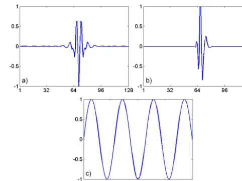
Figure 1. (a) Discretized Meyer basis function for a particular scale and translation; (b) Daubechies (4 tap) basis function with the same scale and translation as (a); (c) a Fourier sinusoid component of the spherical harmonic basis functions. Basis functions are shown normalized to one and are interpolated for ease of viewing.
and the offsetsbˆcan then be recovered as
ˆ
b= BTB−1
BT z−AKxˆ
. (17)
The choice of K has been limited to orthogonal basis func-tions for this paper.
Figure 1 shows a one-dimensional example of the basis functions (normalized to one) that will be used in the ex-periment. Figure 1a and b illustrate two wavelets at the same scale and position for discrete Meyer (DM) and Daubechies 4 (DB4). They have a spatial compact support that makes them particularly useful to resolve localized structures. Figure 1c shows a single harmonic (normalized to one) that has to be multiplied with the Lagrange polynomial (along latitude) to produce a spherical harmonic (SH). They have a longer spa-tial support and work well to describe periodicities in the ionosphere.
2.4 Regularization
Different regularizations exist to stabilize Eq. (15) and make the solution unique and physically meaningful. In this sec-tion the two regularizasec-tions based on the `1 and `2 norm, which are both used for the reconstructions in Sec. 3.1, will be described.
The main goal of regularization is finding the best repre-sentation of the ionosphere that matches the observations and at the same time obviates the lack of data we usually face (e.g. in the oceans between continents).
representation we can have, and its properties will strongly depend on the chosen regularization term.
The`1and`2 regularizations used in this work both aim to create a sufficiently detailed solution by maintaining as much information as possible from the observations. The dif-ference lies in the information that can be extracted from the observations through basis functions and, therefore, on the efficiency on resolving different scale structures. For exam-ple, wavelets are good to localize structures, while spherical harmonics works well with periodicities. Therefore, we are expecting wavelets to resolve better localized structures than spherical harmonics.
The regularization term of Eq. (15) can be expressed in different ways. The classical approach is by using an`2norm (or Tikhonov regularization)
P(x)= kPKxk2
2, (18)
where the matrix P is used to select only a subspace of the possible solutions and stabilize the problem of Eq. (15) to-ward a physically acceptable solution, and the `2 norm is defined as kak2= 2
r P
i
|ai|2. In the implementation of this paper P is set to the identity matrix and the minimization of Eq. (15) with Eq. (18) is solved with the LU decomposition similarly to the framework in Mitchell and Spencer (2003). Another suitable choice of P can be the Laplacian matrix.
A different measure comes from the sparsity which in-volves the number of nonzero coefficients inx (Bruckstein et al., 2009) and is obtained with
P(x)= kKxk0, (19)
wherekak0stands for the number of coefficientsai that are not zero. This approach is particularly suitable for wavelets as it exploits their ability for compact representation. By min-imizing Eq. (15) with Eq. (19) we are looking for the solu-tion which produces the best agreement with the observasolu-tions but that at the same time is also the sparsest one. The min-imization with Eq. (19) is unfortunately not convex, which means that it may have local minima. The complexity of this problem was also proven to be in general not practical as the solution requires to exhaustively search for all the possible combinations of basis functions (the columns in K) that min-imize the functional of Eq. (15) (Natarajan, 1995).
A more feasible solution is obtained with the `1 norm, which in some sense is half way between Eq. (18) and Eq. (19)
P(x)= kPKxk1, (20)
where kak1=P
i
|ai|. The regularization term of Eq. (20) makes the functional Eq. (15) convex and therefore makes it possible to have a unique solution. The solution may differ from the one obtained by Eq. (19), but there are mathematical conditions that ensure Eq. (20) to be equivalent to Eq. (19)
producing an identical solution up to an error term that is proportional to the input noise level (Donoho et al., 2006; Donoho, 2006). The whole theory requires thatx is suffi-ciently sparse, i.e. that the ionosphere can be represented with few basis functions. According to this, sparsity becomes the main goal, allowing better noise removal (i.e. false arte-facts in the reconstruction) but also better compression (e.g. for storing data) in respect to the non-sparse solution (Tsaig and Donoho, 2006; Schmidt, 2007).
The minimization of Eq. (15) with Eq. (20) is implemented with the Fast Iterative Shrinkage-Thresholding Algorithm (FISTA, see Beck and Teboulle, 2009). It applies a non-linear thresholding (or soft-thresholding) (Donoho and Johnstone, 1994) to the estimated coefficientsxˆi at theith iteration η xˆi=
(
0 if xˆi
≤αξ
sgn xˆi
xˆi
−αξ
if xˆi
> αξ
, (21)
whereξ is set to the reciprocal of the maximum eigenvalue of KTATAK and together withαsets the threshold. Then the estimation at the next iteration isxˆi+1=η xˆi
.
A similar stabilization can be introduced by selecting a subset of K by means of a similar thresholding or a greedy subset selection directly applied to Eqs. (15) and (18). This was shown to be not optimal in a general case (Donoho, 2006).
3 Simulation
We selected a grid that spans from North America to Europe. This is a good example to show the limitation imposed, in this case by the ocean, on the density of the receivers. We selected a grid of dimension 64×64 voxels in longitude and latitude, and 22 voxels in altitude. It produces a voxel of di-mension around 1×2◦in latitude and longitude and 50 km in altitude.
Figure 2. Simulated ionosphere with structures added to IRI2012. Values are in TECU (1016electronsperm−2).
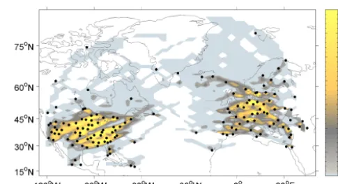
Figure 2 shows the Vertical Total Electron Content (VTEC) map that was used as truth while Fig. 3 illustrates the number of rays that was used in the reconstruction (black dots are the ground stations). The number of rays is obtained by summing the intersections along the altitude within voxels of the grid. The VTEC is calculated by integrating the elec-tron content in a certain latitude and longitude location along the altitude. The ray coverage strictly depends on the density of ground stations, data (STEC) sampling rate and, in our case, the time window within which we run the reconstruc-tion. The selection of the grid is also important as a finer grid will increase the number of voxels that are not intercepted by a ray and the number of coefficients to estimate.
Some structures were located where data coverage is par-ticularly low. In those locations the reconstruction will strug-gle to recover the actual value independently from the reg-ularization that has been used. The behaviour of the algo-rithm in those zones will strongly depend on the regulariza-tion term.
We used EOFs obtained from Chapman profiles (Harg-reaves, 1995), and wavelets (DB4 and DM) and Spherical Harmonics (SH) to represent the horizontal distribution of structures in the ionosphere. By selecting a subset of larger horizontal basis functions we also limited the resolution in the reconstruction, i.e. the smallest scale structures that can be resolved.
For the aim of this paper it will be considered a standard implementation of Eqs. (18) and (20), i.e. the matrix P will be set to the identity matrix.
3.1 Inversion
The reconstructions are shown in Fig. 4 for low resolution and Fig. 5 for high resolution. Each figure shows the be-haviour of the algorithm using different basis functions: SH (top), DM (middle) and DB4 (bottom). In order to high-light the regularization effects where only data coverage was present, we applied a mask (left) to the reconstruction (right). In fact, each regularization technique will handle the absence
Figure 3. Number of rays with ground stations (black dots).
of data in different ways but we want to compare their ability to resolve structures where data are available.
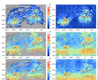
At low resolution the reconstruction looks reasonable for both methods. The structures appear smoothed and with little detail (Fig. 4a, b, c). SH seems to produce some oscillations outside the data coverage (Fig. 4d), mainly in the Atlantic Ocean. This is due to the sinusoidal nature of SH that makes it problematic to represent localized structures. Wavelets do not produce oscillations and the reconstruction looks reason-ably smoothed for this resolution, but there are some edge effects, especially for DM, between Canada and Greenland. Furthermore, DB4 unlike DM tends to fill the data gap in the ocean (Fig. 4f).
Figure 4. Reconstructions obtained at low resolution with masked out VTEC values where there is no ray coverage for (a) spherical harmon-ics; (b) discrete Meyer; (c) Daubechies 4; and without the mask for (d) spherical harmonharmon-ics; (e) discrete Meyer; (f) Daubechies 4. Values are in TECU (1016electronsperm−2).
Figure 5. Reconstructions obtained at high resolution with masked out VTEC values where there is no ray coverage for (a) spherical harmonics; (b) discrete Meyer; (c) Daubechies 4; and without the mask for (d) spherical harmonics; (e) discrete Meyer; (f) Daubechies 4. Values are in TECU (1016electronsperm−2).
Table 1. RMS error (values are in TECU) of the VTEC map obtained with spherical harmonics and wavelets at two different resolutions. Only the VTEC coefficients where there is ray coverage were considered. The percentage of basis functions with non-zero coefficients is also shown and, within brackets, the number in absolute value.
Low resolution High resolution
RMS error Number of basis RMS error Number of basis (TECU) functions (TECU) functions
Spherical harmonics 10.87 100 % (1089) 19.32 100 % (16 641)
Discrete Meyer 6.66 36 % (92) 8.5 8 % (317)
Daubechies 4 7.48 41 % (106) 8.59 11 % (467)
For each reconstruction the root mean square (RMS) error of the VTEC between the true and the reconstructed iono-sphere was calculated. The RMS error is taking into account only the VTEC values where there is ray coverage. Values where there is no ray are, in fact, less meaningful for this statistic.
Table 1 shows the RMS error and the number of basis functions for each reconstruction at the two different resolu-tions. The number of basis functions is shown in percentage and in absolute values within the brackets. The increasing of RMS error with resolution is caused by the attempt of the basis functions to describe the small variations in STEC due to non-uniform data coverage (especially in north Norway). Wavelets need less than 50 % of basis functions at low reso-lution and even less at high resoreso-lution. The small number of basis functions help to stabilize the inversion as only fewer coefficients have to be estimated.
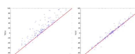
The offsets, obtained from Eq. (14) and averaged for each receiver, are also very well recovered at low resolution by SH (Fig. 6a) and DM (Fig. 6b). Figure 7a and b show the scat-ter plot of the original offsets (xaxis) and the estimated ones (y axis) for each receiver, obtained from the high resolution reconstruction using SH and DM basis functions. At high resolution the offsets are still well estimated from wavelets (Fig. 7b) while they seem to be biased with SH (Fig. 7a). There is in general an overestimation of the offsets that in-creases as the regularization coefficient αincreases. This is due to the fact that whenαincreases, the difference between the observations and the estimation in Eq. (14) increases as well as making the offsets bigger.
3.2 Multi-resolution map
As introduced earlier, another concept that can be exploited with wavelets is multi-resolution analysis. A similar concept was already used in (Schmidt, 2007). Wavelets allow the de-tection of structures according to their scale and position. Small-scale basis functions are therefore selected to repre-sent small variations, otherwise only the basis functions with bigger scales are used. The ability of the algorithm to rec-ognize small variations depends on the data availability and, therefore, the resolution (here intended as the smallest scale
Figure 6. Scatter plot of the estimated offsets (yaxis) versus the true offsets (xaxis) with (a) spherical harmonics and (b) discrete Meyer at low resolution.
Figure 7. Scatter plot of the estimated offsets (yaxis) versus the true offsets (xaxis) with (a) spherical harmonics and (b) discrete Meyer at high resolution.
we can resolve in a certain position in the map) will depend on data.
Figure 8. Multi-Resolution (MR) Map for the high-resolution case with discrete Meyer basis functions. Each box represents the scale of the basis function and its position.
if there is not a comparable (to the scale of the wavelet) en-hancement from the data. This is the case in east and south Europe where, even if good data coverage is provided, only large-scale wavelets are used.
3.3 Noise sensitivity
We stated at the beginning that wavelets allow the better re-moval of noisy terms in the reconstruction. Actually ground stations produce observations that can be considered gener-ally noiseless. The noise term that we intended comes from the fact that the ionosphere is a dynamic medium, where dif-ferent scale structures evolve with time according to compli-cated physics laws in a complex environment.
In order to test the effect of variability in the observations, we decided to add a zero mean Gaussian noise to each ob-servation with a standard deviation of 1 TEC unit. A similar approach was used by Chartier et al. (2012, 2014).
Figure 9a and b show the reconstruction obtained with SH and DM. SH reconstruction (Fig. 9a) is quite sensitive to the noise, which causes additional oscillations and artefacts. DM reconstruction (Fig. 9b) shows a better robustness to noise, and the reconstruction is similar to the ones in Fig. 5e–f. This is mainly due to the sparse regularization which aims to minimize the number of nonzero coefficients. When the soft-thresholding of Eq. (20) is applied with FISTA, a subset of the most significant coefficients is selected. Those coef-ficients will contain the most important part of the energy (or information) (Donoho and Johnstone, 1994). In general, it would not be possible to make the same considerations if the energy was evenly distributed among all the coefficients, like in the case of SH.
The RMS error obtained from Fig. 9a and b is shown also in this case in Table 2 together with the percentage of number of basis functions with non-zero coefficients. The number of basis functions used with DM is slightly decreased compared to the case without noise. This is due to the higher threshold αξ (see Eq. 21) that we used to remove the noise. In the case
Table 2. RMS error (values are in TECU) of the VTEC map ob-tained with spherical harmonics and discrete Meyer with a noise term added to the observations. Only the VTEC coefficients where there is ray coverage were considered. The percentage of basis func-tions with non-zero coefficients is also shown and, within brackets, the number in absolute value.
RMS Number
error of basis (TECU) functions
Spherical harmonics 24.45 100 % (16 641) Discrete Meyer 9.35 7 % (282)
of SH all the basis functions are still used although a higher regularization parameterαwas used too.
3.4 Model-aided inversion
We implemented a model-aided inversion by imaging the residual after removing from the observations a background model of the ionosphere. This is called three-dimensional variational (3DVar) data assimilation and assumes the knowl-edge of a priori information about the state of the iono-sphere. This is generally obtained with an empirical model (like IRI2012) or a first principle physics model. For the sake of this paper we wanted to test the algorithms with Eqs. (18) and (20) under these conditions. Therefore, we considered there was almost perfect knowledge of the ionosphere, i.e. we set the background modeln0to IRI2012 (without the added structures) and considered the residualδn
δn=n−n0. (22)
This residual is associated with a residualδzin the measure-mentszcalculated as
δz=z−An0. (23)
Therefore, the problem in Eq. (15) becomes
F (δx)= kδz−AKδxk2C+αP(δx) , (24) whereδx= KTK−1KTδn. Hence, the inverse problem is applied to Eq. (24), which will calculate the residual informa-tion that the a priori model could not reproduce (in this case the structures added to IRI2012). The final reconstruction is obtained by summing the estimated δnˆ to the background modeln0. To make the problem more difficult we also added the noise term into the datazas in the previous section. The reconstruction (plus background model) is shown in Fig. 10a and b for SH and DM.
Figure 9. Reconstruction with (a) spherical harmonics and (b) discrete Meyer at high resolution with Gaussian noise added to the observa-tions. The Gaussian noise has zero mean and a standard deviation of 1 TEC unit.
Figure 10. Model-aided reconstruction obtained with (a) spherical harmonics and (b) discrete Meyer at high resolution. A noise term (zero-mean Gaussian with 1 TEC unit of standard deviation) was added to the observations.
Table 3. RMS error (values are in TECU) of the VTEC map ob-tained with a 3DVar scheme using spherical harmonics and discrete Meyer with a noise term added to the observations. Only the VTEC coefficients where there is ray coverage were considered. The per-centage of basis functions with non-zero coefficients is also shown and within brackets the number in absolute value.
RMS Number
error of basis (TECU) functions
Spherical harmonics 9.26 100 % (16 641) Discrete Meyer 8.66 7.3 % (300)
By perfectly removing the background the algorithm needs to resolve only few relatively smooth structures at a different scale. This scenario can be considered as the best case, where we had background knowledge of the iono-sphere, in comparison with the worst case of the previous subsection where such knowledge was lacking. Actually, we will never have a perfect knowledge of the ionosphere and, therefore, a background model cannot aid the reconstruction as in the above example. This mismatching with the truth means that the algorithm with an approximated background model will have performances between the worst and best case.
4 Conclusions
Sparse regularization has been shown to be a valid alternative to standard method based on Tikhonov regularization and is particularly suitable with wavelets.
increases considerably. We have shown tomographic recon-structions obtained with Spherical Harmonics (SH) and two different wavelets, Daubechies 4 (DB4) and Discrete Meyer (DM) in a worst and best case. The best case was obtained by selecting a background model which exactly represented the smoothed ionosphere, whilst the worst case was without any background model. In both cases wavelets were shown to produce the best reconstruction in terms of the root mean square (RMS) error and oscillations (artefacts). An important characteristic in this new approach is the ability of wavelets to handle the uneven distribution of the observations. We have explained this ability through the multi-resolution map showing how the resolution is adapted to the data cover-age and the ionospheric structures observed by the measure-ments.
It is noted that CIT is actually a time-dependent inversion problem and in this paper it has been simplified in the simula-tion to a case where the ionosphere does not change in time. The work in this paper has shown the potential of the method when the ionosphere does not considerably change within a short time window, e.g. under quiet geomagnetic conditions. For more active conditions a full 4-D imaging would be re-quired. This factor will be studied in further research.
In conclusion sparse regularization techniques can pro-duce significant improvements to CIT and to inverse prob-lems in general. They demonstrate properties of noise ro-bustness and adaptability to data coverage. The choice of wavelet basis functions is not critical, but we believe that other wavelet constructions could lead to further improve-ments.
Acknowledgements. We thank the International Reference
Iono-sphere (IRI) project (http://iri.gsfc.nasa.gov/) and the UNAVCO and IGS repositories for offering free access to GPS data. This research activity was funded by the European Union’s Seventh Framework Programme for research, technological development and demonstration under grant agreement no. 264476.
Edited by: G. Lapenta
Reviewed by: two anonymous referees
References
Amerian, Y., Hossainali, M. H., Voosoghi, B., and Ghaffari, M. R.: Tomographic Reconstruction of the Ionospheric Electron Den-sity in term of Wavelets, Journal of Aerospace Science and Tech-nology, 7, 19–29, 2010.
Beck, A. and Teboulle, M.: A fast iterative shrinkage-thresholding algorithm for linear inverse problems, SIAM Journal on Imaging Sciences, 2, 183–202, 2009.
Bruckstein, A. M., Donoho, D. L., and Elad, M.: From Sparse So-lutions of Systems of Equations to Sparse Modeling of Signals and Images, SIAM Review, 51, 34–81, doi:10.1137/060657704, 2009.
Chapman, S.: The absorption and dissociative or ionizing effect of monochromatic radiation in an atmosphere on a rotating earth, P. Phys. Soc., 43, 26–45, 1931.
Chartier, A. T., Mitchell, C. N., and Jackson, D. R.: A 12 year comparison of MIDAS and IRI 2007 ionospheric Total Electron Content, Adv. Space Res., 49, 1348–1355, doi:10.1016/j.asr.2012.02.014, 2012.
Chartier, A. T., Kinrade, J., Mitchell, C. N., Rose, J. A. R., Jack-son, D. R., Cilliers, P., Habarulema, J.-B., Katamzi, Z., McKin-nell, L.-A., Matamba, T., Opperman, B., Ssessanga, N., Giday, N. M., Tyalimpi, V., Franceschi, G. D., Romano, V., Scotto, C., Notarpietro, R., Dovis, F., Avenant, E., Wonnacott, R., Oyeyemi, E., Mahrous, A., Tsidu, G. M., Lekamisy, H., Olwendo, J. O., Sibanda, P., Gogie, T. K., Rabiu, B., Jong, K. D., and Ade-wale, A.: Ionospheric imaging in Africa, Radio Sci., 49, 19–27, doi:10.1002/2013RS005238, 2014.
Daubechies, I., Defrise, M., and De Mol, C.: An iterative thresh-olding algorithm for linear inverse problems with a spar-sity constraint, Commun. Pur. Appl. Math., 57, 1413–1457, doi:10.1002/cpa.20042, 2004.
Davies, K.: Ionospheric Radio, in: Ieee Electromagnetic Waves Se-ries (Book 31), The Institution of Engineering and Technology, London, 1990.
Dear, R. M. and Mitchell, C. N.: GPS interfrequency biases and total electron content errors in ionospheric imaging over Europe, Radio Sci., 41, RS6007, doi:10.1029/2005RS003269, 2006. Donoho, D. L.: For most large underdetermined systems of
linear equations the minimal `1-norm solution is also the sparsest solution, Commun. Pur. Appl. Math., 59, 797–829, doi:10.1002/cpa.20132, 2006.
Donoho, D. L. and Johnstone, I. M.: Threshold selection for wavelet shrinkage of noisy data, in: Engineering in Medicine and Biol-ogy Society, 1994. Engineering Advances: New Opportunities for Biomedical Engineers. Proceedings of the 16th Annual In-ternational Conference of the IEEE, 3–6 November 1994, Balti-more, MD, A24–A25, 1994.
Donoho, D. L., Elad, M., and Temlyakov, V. N.: Sta-ble recovery of sparse overcomplete representations in the presence of noise, IEEE T. Inform. Theory, 52, 6–18, doi:10.1109/TIT.2005.860430, 2006.
Durmaz, M. and Karslio˘glu, M. O.: Non-parametric regional VTEC modeling with Multivariate Adaptive Regression B-Splines, Adv. Space Res., 48, 1523–1530, doi:10.1016/j.asr.2011.06.031, 2011.
Fremouw, E. J., Secan, J. A., and Howe, B. M.: Application of stochastic inverse theory to ionospheric tomography, Radio Sci., 27, 721–732, doi:10.1029/92RS00515, 1992.
Hargreaves, J. K.: The Solar-Terrestrial Environment: An Introduc-tion to Geospace – The Science of the Terrestrial Upper sphere, Ionosphere, and Magnetosphere, in: Cambridge Atmo-spheric and Space Science Series, Cambridge University Press, New York, 1995.
Jakowski, N.: TEC monitoring by using satellite positioning sys-tems, in: Modern Ionospheric Science – 50 Years of Ionospheric Research in Lindau, edited by: Kohl, H., Rüster, R., and Schlegel, K., Produserv GmbH Verlagsservice, Germany, 371–389, 1996. Loris, I., Douma, H., Nolet, G., Daubechies, I., and Regone, C.:
J. Comput. Phys., 229, 890–905, doi:10.1016/j.jcp.2009.10.020, 2010.
Mannucci, A. J., Iijima, B. A., Lindqwister, U. J., Pi, X., Sparks, L., and Wilson, B. D.: GPS and ionosphere, in: Review of Radio Science (1996–1999), edited by: Ross Stone, W., Wiley-IEEE Press, New York, 625–665, 1999.
Mitchell, C. N. and Spencer, P. S. J.: A three-dimensional time-dependent algorithm for ionospheric imaging using GPS, Annals of Geophysics, 46, 10 pp. doi:10.4401/ag-4373, 2003.
Na, H. and Lee, H.: Analysis of fundamental resolution limit of ionospheric tomography, in: Acoustics, Speech, and Signal Pro-cessing, 1992. ICASSP-92., 1992 IEEE International Conference on, 23–26 March 1992, San Francisco, CA, 97–100, 1992. Natarajan, B. K.: Sparse Approximate Solutions to
Linear Systems, SIAM J. Comput., 24, 227–234, doi:10.1137/S0097539792240406, 1995.
Schmidt, M.: Wavelet modelling in support of IRI, Adv. Space Res., 39, 932–940, doi:10.1016/j.asr.2006.09.030, 2007.
Schmidt, M., Bilitza, D., Shum, C., and Zeilhofer, C.: Regional 4-D modeling of the ionospheric electron density, Adv. Space Res., 42, 782–790, doi:10.1016/j.asr.2007.02.050, 2008.
Simons, F. J., Loris, I., Nolet, G., Daubechies, I. C., Voronin, S., Judd, J. S., Vetter, P. A., Charléty, J., and Vonesch, C.: Solving or resolving global tomographic models with spherical wavelets, and the scale and sparsity of seismic heterogeneity, Geophys. J. Int., 187, 969–988, doi:10.1111/j.1365-246X.2011.05190.x, 2011.
Spencer, P. S. J. and Mitchell, C. N.: Imaging of 3-D plasmaspheric electron density using GPS to LEO satel-lite differential phase observations, Radio Sci., 46, RS0D04, doi:10.1029/2010RS004565, 2011.
Sutton, E. and Na, H.: High resolution ionospheric tomography through orthogonal decomposition, in: Image Processing, 1994. Proceedings. ICIP-94, IEEE International Conference, 13–16 November 1994, Austin, TX, 148–152, 1994.
Tikhonov, A. N. and Arsenin, V. Y.: Solution of ill-posed prob-lems, Scripta series in mathematics, Winston & Sons, Washing-ton, D.C., 258 pp., 1977.
Tsaig, Y. and Donoho, D. L.: Breakdown of equivalence between the minimal`1-norm solution and the sparsest solution, Signal Process., 86, 533–548, doi:10.1016/j.sigpro.2005.05.028, 2006. Yeh, K. C. and Raymund, T. D.: Limitations of
iono-spheric imaging by tomography, Radio Sci., 26, 1361–1380, doi:10.1029/91RS01873, 1991.
Zeilhofer, C., Schmidt, M., Bilitza, D., and Shum, C.: Re-gional 4-D modeling of the ionospheric electron density from satellite data and IRI, Adv. Space Res., 43, 1669–1675, doi:10.1016/j.asr.2008.09.033, 2009.