www.nonlin-processes-geophys.net/22/275/2015/ doi:10.5194/npg-22-275-2015
© Author(s) 2015. CC Attribution 3.0 License.
Oscillations in a simple climate–vegetation model
J. Rombouts1and M. Ghil2,3
1Centre for Complexity Science, University of Warwick, Coventry, UK
2Geosciences Department and Environmental Research & Teaching Institute, Ecole Normale Supérieure, Paris, France 3Atmospheric & Oceanic Sciences Department and Institute of Geophysics & Planetary Physics, University of California, Los Angeles, CA, USA
Correspondence to: J. Rombouts ([email protected])
Received: 21 November 2014 – Published in Nonlin. Processes Geophys. Discuss.: 2 February 2015 Revised: 12 April 2015 – Accepted: 17 April 2015 – Published: 7 May 2015
Abstract. We formulate and analyze a simple dynamical sys-tems model for climate–vegetation interaction. The planet we consider consists of a large ocean and a land surface on which vegetation can grow. The temperature affects vegeta-tion growth on land and the amount of sea ice on the ocean. Conversely, vegetation and sea ice change the albedo of the planet, which in turn changes its energy balance and hence the temperature evolution. Our highly idealized, conceptual model is governed by two nonlinear, coupled ordinary dif-ferential equations, one for global temperature, the other for vegetation cover. The model exhibits either bistability be-tween a vegetated and a desert state or oscillatory behavior. The oscillations arise through a Hopf bifurcation off the veg-etated state, when the death rate of vegetation is low enough. These oscillations are anharmonic and exhibit a sawtooth shape that is characteristic of relaxation oscillations, as well as suggestive of the sharp deglaciations of the Quaternary.
Our model’s behavior can be compared, on the one hand, with the bistability of even simpler, Daisyworld-style climate–vegetation models. On the other hand, it can be in-tegrated into the hierarchy of models trying to simulate and explain oscillatory behavior in the climate system. Rigorous mathematical results are obtained that link the nature of the feedbacks with the nature and the stability of the solutions. The relevance of model results to climate variability on vari-ous timescales is discussed.
1 Introduction 1.1 Background
Climate has an important effect on vegetation. Plant growth is affected by temperature, carbon dioxide (CO2) levels and nutrient availability. The space available for growth matters as well: ice-covered parts of land are not suitable for it. The interaction also works the other way around, though: vege-tation plays an important role in climate regulation. Many different effects are at play, with the albedo being one of the most important ones: vegetation is darker than bare ground or ice and therefore absorbs more solar radiation and warms the planet.
This vegetation–albedo feedback appears to be important in semi-arid regions (Otterman, 1974), where it interacts with the hydrological cycle. J. G. Charney and colleagues (Char-ney, 1975; Charney et al., 1975) were the first to include in a model this biogeophysical feedback, as he called it; many others have followed since (Claussen et al., 1999; Zeng et al., 1999; Zeng and Neelin, 2000). The vegetation–albedo feed-back also matters in certain high-latitude regions (Otterman et al., 1984), where boreal forests mask snow in winter, caus-ing an effective warmcaus-ing of the surface (Brovkin et al., 2003; Bonan, 2008).
initials of the original authors (Charlson et al., 1987; Ayers and Cainey, 2007) – evapotranspiration or more exotic feed-backs, such as the so-called lightning–biota feedback (She-pon and Gildor, 2008). Meir et al. (2006) review several im-portant mechanisms by which terrestrial ecosystems affect climate, while Claussen (2009) provides an introduction to vegetation–climate interactions on paleoclimate timescales.
Although vegetation plays an essential role in the climate system, it has only been rather recently included as an active player in climate models. The hierarchy of climate models (Schneider and Dickinson, 1974; Ghil and Robertson, 2000; Ghil, 2001) ranges from simple, conceptual ordinary differ-ential equation (ODE) models – through intermediate models of varying complexity – all the way up to full-scale general circulation models or global climate models (GCMs). Across this whole range, vegetation can be included to better ex-plain various climatic phenomena and trends. In some cases, the predictions of models that couple atmosphere, ocean and vegetation dynamics – often referred to as Earth system mod-els (ESMs) – differ radically from modmod-els that exclude the vegetation (Meir et al., 2006). It follows that it is of the essence to include vegetation in our models to obtain a better understanding of climate evolution and variability.
The simplest climate models are conceptual models, which are usually governed by a small number of ODEs. These models do not claim to be realistic in the sense of mak-ing precise quantitative predictions, but allow one to study basic underlying mechanisms. They are also useful for ex-ploring qualitative changes in the climate system’s behavior, commonly known in dynamical systems theory as bifurca-tions (Ghil and Childress, 1987; Dijkstra and Ghil, 2005), and related more recently to the broader and fuzzier concept of “tipping points” (Lenton et al., 2008). Bifurcations or tip-ping points correspond to situations in which a small param-eter change can have a large effect on the behavior of the whole system.
Studying conceptual models can also provide guidance in interpreting results from larger, more detailed models (Brovkin et al., 1998, 2003; Ghil and Robertson, 2000). Early applications of dynamical systems theory and of numerical bifurcation studies to the climate system included H. Stom-mel’s bistability study of the thermohaline circulation (Stom-mel, 1961) and E. N. Lorenz’s study of chaos in a simple con-vection model (Lorenz, 1963). Another such application was to explain Quaternary glaciation cycles as climatic-oscillator solutions (Källèn et al., 1979; Le Treut and Ghil, 1983; Saltz-man, 1983; Ghil and Childress, 1987; Ghil, 1994; Crucifix, 2012).
In the latter idealized climate-oscillator models, vegeta-tion is not usually included. There are, however, some simple models that explore the interaction between climate and veg-etation, and we will briefly review some noteworthy ones in the next section.
1.2 Simple ODE models for climate–vegetation feedbacks
A pioneering model dealing with vegetation and climate was Daisyworld (Watson and Lovelock, 1983). This model illus-trates how vegetation may act to regulate planetary tempera-ture through the albedo feedback, for a wide range of param-eter values. The varying paramparam-eter is in this case the incom-ing solar radiation. The model has been thoroughly studied and extended; see the review of Wood et al. (2008).
Svirezhev and von Bloh (1996, 1997) introduced an-other set of simple, spatially zero-dimensional (0-D) mod-els for vegetation–climate interactions. These highly simpli-fied models include an ODE for temperature evolution, ab-sent from Daisyworld, but look at only one type of vegeta-tion, whereas Daisyworld has two. In their two-ODE model, Svirezhev and von Bloh (1996) find multiple steady states. Such bistability seems to occur across a hierarchy of climate– vegetation models, from the simplest (Dekker et al., 2007; Janssen et al., 2008; Aleina et al., 2013) to more complex (Brovkin et al., 1998; Claussen, 1998; Irizarry-Ortiz et al., 2003; Renssen et al., 2003) ones, although it is, of course, harder to ascertain in the latter. In models across the hi-erarchy, vegetation and temperature are often coupled with precipitation, which provides an additional feedback mecha-nism.
Beyond the possibility of multiple steady states, it is of in-terest to examine in the simplest conceptual models the pos-sibility of internal, self-sustained oscillations. Oscillatory be-havior has been observed in Daisyworld-like models, for ex-ample when an explicit temperature equation is added (Nevi-son et al., 1999; Fernando Salazar and Poveda, 2009), or when delays are introduced (De Gregorio et al., 1992).
So far, though, simple, 0-D climate–vegetation models seem not to have included an ocean component. Earth’s oceans constitute about 70 % of the area of the planet, and are a very important factor in determining its climate (Stom-mel, 1961; Saltzman, 1983; Ghil, 1994; Dijkstra and Ghil, 2005). The global ocean is often included in 0-D paleocli-mate models for glacial cycles (Källèn et al., 1979; Le Treut and Ghil, 1983; Ghil and Childress, 1987; Gildor and Tziper-man, 2001; Crucifix, 2012). Our model will include an ocean and the associated sea ice, and will combine certain features of Daisyworld-like models and climatic-oscillator models.
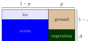
ocean
vegetation ground ice
1−p p
A 1−A
Figure 1. Schematic representation of the model planet’s surface, including a fractionpof land and 1−pof ocean. The fraction of the ocean that is covered by sea ice depends on the global tempera-tureT, while the land is covered by a fractionAof vegetation.
2 Model description
The climate system contains several subsystems, all work-ing together to produce highly nonlinear behavior through its many feedback mechanisms. Some of the simplest and most important feedback effects act via the planetary albedo: darker areas – like the vegetated ones – absorb more so-lar energy and thus warm the planet, while lighter areas – such as those covered by snow and ice – tend to cool it. The ice–albedo feedback was included in energy balance models (EBMs) of climate long ago (Budyko, 1969; Sellers, 1969), and a vegetation–albedo feedback regulates Daisyworld’s be-havior. The latter will constitute the main mechanism in our present model.
The model’s two governing equations are given below:
CT dT
dt =(1−α(T , A)) Q0−Ro(T ), (1a)
dA
dt =β(T )A(1−A)−γ A. (1b)
The variableT denotes global average temperature, whileA
denotes the fraction of land that is covered by vegetation. TemperatureT changes in Eq. (1a) as a result of the bal-ance between incoming and outgoing energy. The parame-terQ0is the incoming solar energy, which is equal here to 342.5 Wm−2. The functionα=α(T,A) denotes the depen-dence of the albedo onT andA, and it is given by
α=(1−p)αo(T )+p αvA+αg(1−A), (2) where p is the fraction of the planet that is land, taken to be 0.3 like on Earth.
The valuesαo,αvandαgdenote the albedo of the ocean, of the vegetation and of bare ground, respectively. The latter two are constant, and an essential ingredient of our model is thatαv< αg, i.e., that forests and savannas are darker and absorb more energy than bare ground.
The albedo of the ocean will be taken as a function of global temperatureT, to account for the possible presence of sea ice. We will use a ramp function, as in Sellers (1969) and Ghil (1976). This function is given by the following equa-tion:
0 0.5
1
Tα,` Temperature
Fraction
of
sea
ice
0 0.2
0.4
0.6
0.8 1
Tα,u αmax
αmin
Ocean
alb
edo
Figure 2. Fraction of sea ice cover (blue) and ocean albedo (red) as a function of temperatureT. The ocean albedo is a weighted average of the albedo of open water and of ice, and is therefore directly dependent on the fraction of sea ice.
αo(T )=
αmax if T≤Tα,`,
αmax+αTminα,u−−αTmaxα,` T−Tα,`
if Tα,`< T≤Tα,u,
αmin if Tα,u< T .
(3)
Hereαmax=0.85 for the ice-covered ocean,αmin=0.25 for the ice-free ocean,Tα,`=263 K andTα,u=300 K. The value ofTα,uis rather high – almost 27◦C – which means that a tiny bit of sea ice will be present even for very high global temperature. Figure 1 shows a schematic representation of our planet’s surface features and a plot of the ocean albedo versus temperature is shown in Fig. 2.
The function Ro(T ) denotes the energy outgoing from the planet. Several EBMs have used a modified version of the quartic Stefan–Boltzmann law (Sellers, 1969; Ghil, 1976), while other such models have used a linearization thereof (Budyko, 1969). We will also use here a linear de-pendence of outgoing radiation on temperature, but radia-tion increases in it more slowly with temperature than in the Stefan–Boltzmann case. This slower increase takes into ac-count the fact that increasing temperature entrains increasing CO2 levels and thus an increased greenhouse effect, which tends to decrease the outgoing radiation.
The form ofRo(T )we choose is
Ro(T )=B0+B1 T −Topt, (4) whereB0 and B1 are constants, while Topt is the optimal growth temperature for the vegetation. There is a huge uncer-tainty in the values of these parameters, especially inB1, the linearized effect of temperature on radiative forcing (IPCC, 2013), since it all depends on which effects are taken into account and which are not (Zaliapin and Ghil, 2010).
Table 1. Definition and values of the model parameters.
Symbol Meaning Value
CT Heat capacity 500 W yr K−1m−2
Q0 Incoming solar energy 342.5 W m−2
p Fraction of land 0.3
αv Albedo of vegetation 0.1
αg Albedo of ground 0.4
αmax Albedo of ice-covered ocean 0.85
αmin Albedo of ice-free ocean 0.25
Tα,` Temperature below which ocean is ice-covered 263 K
Tα,u Temperature above which ocean is ice-free 300 K
B0 Constant in outgoing radiation 200 W m−2
B1 Constant in outgoing radiation 2.5 W K−1m−2
Topt Optimal growth temperature 283 K
k Parameter for width of growth curve 0.004 yr−1K−2
γ Death rate of vegetation 0.1 yr−1
we are interested in – they correspond rather well to a lin-earization of an outgoing energy term of the formgσ T4with
g=0.55, wheregis a constant denoting the grayness of the atmosphere (see Fig. 3). Such a parametrization of outgo-ing energy – the Stefan–Boltzmann law with a multiplicative factor – is often used, but usually g is allowed to depend on another variable, such as temperature (Sellers, 1969) or CO2level (Svirezhev and von Bloh, 1997), rather than being merely a constant, as in Fig. 3 here.
Vegetation cover Ain Eq. (1b) grows logistically, with a temperature-dependent growth rate β(T ). The shape of the functionβfollows Daisyworld and related models, to wit,
β(T )=maxn0,1−k T−Topt2
o
. (5)
This means that the growth rate is zero, except for a certain interval, in which the dependence is parabolic with a maxi-mum atTopt, which is 283 K in our model.
The parameterγ is the mean death rate of the global vege-tationA, and its value is, at first, set to 0.1 yr−1. Table 1 lists the definition of the model parameters and their nominal val-ues. In Sect. 3.2,γ will serve as a control parameter in our exploration of model behavior.
3 Analytical and numerical results 3.1 Multiple equilibria and their stability
We start, as usual, by looking at the fixed points of the sys-tem (Eq. 1), and will use, again as usual, interchangeably the terms steady states, stationary solutions and equilibria. One obvious fixed point is given byA=A0=0, with temperature
T0given by the solution ofQ0(1−α(T0, 0))=Ro(T0). For our parameter values, a solutionT0only exists whenT < Tα,` and it equalsT0'243 K.
260 270 280 290 300 310 320 150
200 250 300
Temperature (K)
Outgoing
energy
(W/m
2)
Our model
Ro(T) =gσT4
Figure 3. Outgoing energy as a function of temperature for different parametrizations.
This result implies that a planet without vegetation will necessarily drop into a very cold “snowball-Earth” state. Note that this result differs from that of EBMs with no veg-etation, in which two stable fixed points co-exist for suf-ficiently high Q0 (North et al., 1981; Ghil and Childress, 1987).
260 270 280 290 300 310 320 0
0.2
0.4 0.6 0.8
1
Temperature (K)
V
egetation
co
ver
Figure 4. The (T,A) phase plane of the model, with the two null isoclines given by Eq. (6) (red straight line) and Eq. (7) (blue curve), respectively. The fixed points for the vegetated states of our planet are the intersections of these two curves. The non-vegetated fixed point forA6=0 does not appear in this plot.
In the presence of vegetation, A6=0, a fixed point (T+,
A+) must satisfy
A+=1−
γ β (T+)
, (6)
according to the vegetation equation (Eq. 1b). From the tem-perature equation (Eq. 1a), we see furthermore that, at a fixed point, one also has
A+= 1 αv−αg
1
p
1−Ro(T+) Q0
−(1−p)αo(T+)
−αg
. (7)
The two curves in the phase plane (T,A) of the model that are given by Eqs. (6) and (7) are called the null isoclines – or nullclines, for short – of the system, and they are plotted in Fig. 4. They intersect at two points, aside from the previously discussed bare-land solution; hence, we have two additional equilibria for a vegetated planet.
To study the stability of these fixed points, we consider the Jacobian matrix J=J(T,A) for the system Eq. (1),
J= a
−1
CTQ0
∂α ∂A ∂β
∂TA(1−A) β(T )(1−2A)−γ
!
, (8)
where
a=−1
CT
Q0
∂α ∂T +
∂Ro
∂T
. (9)
For the no-vegetation fixed pointA=0, the eigenvalues of J(T, 0) areaandβ(T )−γ. These eigenvalues are both neg-ative, sinceT is so low at this fixed point that∂α/∂T=0 and
β(T )=0. Hence, this non-vegetated state is always linearly stable.
240 260 280 300 320
0 0.5
1 1.5
Temperature (K)
V
egetation
co
ver
Figure 5. The model’s phase plane with the two nullclines (dashed lines) and the three fixed points (open and filled dots); the two filled dots are stable, while the open one is unstable. The stable manifold of the saddle (open dot) is shown in black and the unstable one in magenta. The coordinates of the fixed points are (242.04, 0) for the unvegetated state, and (280.8, 0.898) and (297.9, 0.129) for the unstable and stable vegetated states, respectively.
Let us now look at the other two fixed points, shown in Fig. 4, where A >0. Note that since A=1−γ /β(T ), the temperature must be in the range whereβ(T ) >0. With our choice of parameters, this range also lies in the interesting range betweenTα,`andTα,u, within which we have sea ice feedback; it corresponds to the decreasing part of the temper-ature nullcline, given by Eq. (7), and shown as the dashed red line in Fig. 5.
The leftmost of these two fixed points, whereA >0, is a saddle. This can be seen from numerical computations, but we can also deduce it analytically. In the following, we will useβ0 instead of ∂β/∂T, since the function β depends on temperature alone, and no confusion can arise. We have the following proposition.
Proposition 1. A climate–vegetation fixed point (T+,A+),
whereA+>0, is a saddle, and hence unstable, if the
vege-tation growth rateβ(T )is an increasing function of global temperatureT,β0(T+) >0.
The proof is given in Appendix A, and it does not de-pend on any particular parameter values, only on their rel-ative signs; nor is the exact parametrization of the growth rateβused.
For the stability of the latter, rightmost fixed point, Propo-sition 1 above says nothing, sinceβ0(T ) <0 there. Numeri-cal computation shows that the eigenvalues of the Jacobian J(T, A) at this point are complex conjugate and equal to
λ±= −0.006±0.028i. Hence, the fixed point is a focus and
the real partλr=tr(J)/2, where tr(J) is the trace of the Jaco-bian matrix, is negative; thus the focus is stable.
We can compute the trace of J analytically:
tr(J)=a+β(T )(1−2A)−γ=a−β(T )+γ=a+x. (10) The term a on the right-hand side is larger than 0, but the termx=γ−β(T )compensates and, for the standard param-eter values in Table 1, tr(J) is negative, implying the stability of the focus. One suspects, however, that, as some of these parameter values change, the focus may lose its stability.
We investigate next this loss of stability and the more com-plex model behavior to which it leads.
3.2 Hopf bifurcation and oscillatory behavior 3.2.1 Analytical results
We study now in greater detail the stability of the fixed point with non-zero vegetation (T+,A+). The result is stated in
the following proposition and the proof thereof is given in Appendix A, after the one for Proposition 1.
Proposition 2. A model fixed point (T+,A+) that lies in
the region with active sea ice feedback (Tα,`< T+< Tα,u) is a focus if and only if the following inequality holds:
(1−y)2<4η(y)y, (11) wherey=(γ−β(T+))/a,η(y)is (up to a sign change) the
ratio of the derivatives of the two nullclines and a is given by Eq. (9).
Given the inequality (Eq. 11), the focus is stable ify <−1. The proof in the Appendix relies simply on rewriting the classic conditions on the Jacobian.
We know thaty <0, sincex <0 andais positive, and also thatη(y)is always negative. Since for all negativeywe have
(1−y)2>4|y|,
a necessary condition to have a focus is that|η|>1, i.e., that the ratio of the derivatives of the nullclines should be large enough in absolute value.
The proof of Proposition 1 in the Appendix implies, how-ever, that this condition is already necessary for a fixed point to not be a saddle. Since the temperature nullcline is a piece-wise linear curve, its derivative is a constant and a focus can only occur when the vegetation nullcline is steep enough. This condition, in turn, corresponds to the vegetation cover
A+ being small enough, as can be seen in the phase plane
plotted in Fig. 5. It follows that a Hopf bifurcation and, there-fore, oscillations, can only occur around a model state with
0 0.1 0.2 0.3 0.4 0.5
0 0.2
0.4
0.6
0.8
1
Saddle-node bifurcation
Hopf bifurcation
γ
V
egetation
co
ver
stable unstable
Figure 6. Bifurcation diagram, with the vegetationAplotted ver-sus the death rate γ. The branches were computed using the XPPAUT software package (Ermentrout, 2002).
low vegetation. Since we did not use the actual value of any of the parameters, this result is quite general.
As shown in the caption of Fig. 5, the temperature value for the vegetated fixed point isT+=297.9. The
correspond-ing value ofyis−1.96. The ratioη(y)of the nullcline slopes equals−9.6; hence|η(y)|>1, and thus the point could be a focus. Substituting in Eq. (11) yields 8.75<75.17, which shows that the inequality is satisfied and that this point is a focus. Sincey= −1.96<−1, the focus is stable.
3.2.2 Numerical results
As announced at the end of Sect. 2, we now vary the death rateγ of the vegetation and follow the change in model solu-tions. For decreasingγ, i.e., for longer-lived vegetation, the focus loses its stability and the associated Hopf bifurcation gives rise to a limit cycle, as shown in the bifurcation diagram of Fig. 6. This bifurcation occurs forγ=0.02572, i.e., when the overturning time 1/γ of the vegetation is about 40 years, which corresponds definitely to trees rather than grasses.
We can also see in Fig. 6 that, whenγis higher than 0.41, non-zero vegetation can no longer be a steady-state solution. At γ'0.41, a saddle-node bifurcation gives rise to a sta-ble (blue curve) and an unstasta-ble (red curve) branch of steady states, in addition to the stable branchA≡0 studied in the previous subsection and not shown in the figure.
We mentioned in Sect. 3.1 above that the parameter change needs to make tr(J) positive in order to change the stabil-ity. This also works if, instead of decreasingγ, we decrease the thermal heat capacityCT. It is the productγ CTthat de-termines the behavior of the system, not the two parameters separately.
0 500 1,000 1,500 2,000 2,500 3,000 3,500 4,000 4,500 5,000 0
0.5
Time (years)
V
egetation
co
ver
296 298 300 T
emp
eratur
e
(K)
0 500 1,000 1,500 2,000 2,500 3,000 3,500 4,000 4,500 5,000 0
0.05 0.1
Time (years)
Fraction
sea
ice
(a)
(b)
Figure 7. Typical oscillatory model solution, shown here forγ=0.02; i.e.,γ /CT=1/10. (a) Temperature and vegetation cover; and (b)
frac-tion of the ocean that is covered by sea ice. The period of these regular oscillafrac-tions is a little under 1000 years.
instance, in the temperature–ice sheet oscillator of Källèn et al. (1979), the characteristic time of ice sheet evolution
CLshould be large enough in comparison with the timescale
CTassociated with the thermal inertia of the oceans; see Ghil and Tavantzis (1983).
Nevison et al. (1999) also obtained certain results that are somewhat similar to ours. Their paper explores a Daisyworld with an equation for temperature evolution. The system ex-hibits self-sustained oscillations for a certain range ofCTand
γ, just like in our model. The albedo feedback in this model is due to two types of daisies, black (absorbing) and white (reflecting) ones. The bimodality of the albedos in both mod-els leads us to suspect that the role of sea ice in our model corresponds roughly to that of the white daisies in the model by Nevison and colleagues.
This analogy should not be pushed too far, however. White daisy growth is favored by warmer temperatures, whereas sea ice appears at low temperatures. A comparison between our Fig. 7 and Fig. 2 in Nevison et al. (1999) shows that the be-havior of black daisies and temperature is analogous to our vegetation and temperature, while increases in sea ice and white daisies have a different phase. The former occurs with decreasing temperature, while the latter happens as tempera-ture increases.
Another interesting difference between the two models lies in the value ofγfor which oscillations are obtained. We have 1/γ'40 yr, while Nevison and colleagues obtain the oscil-lations when 1/γ is of the order of a few months, with a similar value of CT. The difference probably resides in the nature of the feedback: in our model, the ocean and sea ice play a role, with both operating on seasonal and interannual timescales. In the Nevison et al. (1999) model, it is two kinds
of daisies on an all-land planet that interact, both with much shorter timescales.
Oscillatory behavior is also observed in the Daisyworld variant studied by De Gregorio et al. (1992). In their paper, an explicit delay is introduced into the Daisyworld system. When the delay is long enough, oscillations are observed. This again shows the importance of timescales in these oscil-lations. The mechanism by which the oscillations arise in the delayed system of De Gregorio and colleagues is also shown to be a Hopf bifurcation, like in delayed, spatially dependent EBMs (Bhattacharya et al., 1982; Roques et al., 2014) and in certain simple and intermediate models of the El Niño– Southern Oscillation (ENSO) (Jin et al., 1994; Tziperman et al., 1994; Ghil et al., 2008, and references therein).
This again shows the importance of timescales: only when the effect of temperature on the growth rate of the vegetation is substantially delayed does the system exhibit internal os-cillations. The discussion on timescales in Daisyworld is the subject of a recent paper by Weaver and Dyke (2012), where the persistency of regulatory behavior under a separation of timescales is examined.
Figure 7 (upper panel) shows plots of temperature (red curve) and vegetation cover (blue curve) versus time. The oscillations have an amplitude of a few degrees for the tem-perature, but are very large for the vegetation, going from almost no vegetation to 70 % of the land being covered by plants. In addition, the vegetation plot shows a sawtooth-like shape, with the vegetation cover almost vanishing for long times, after which it shoots back up.
This behavior has been modeled using relaxation oscilla-tions; cf. Le Treut and Ghil (1983), Ghil (1994) and Crucifix (2012), among others. In these studies, the sawtooth shape is due to a quick melting and slow build-up of the ice sheets, whereas in Gildor and Tziperman (2001), the sea ice plays a key role. In the intermediate-complexity model of Ganopol-ski and Calov (2011), like in the early conceptual model of Imbrie and Imbrie (1980), it is the strongly nonlinear re-sponse of the climate–cryosphere system to orbital forcing. In the present model, it is the surge in vegetation growth ac-companying a temperature rise that provides the characteris-tically asymmetric nature of the oscillation.
Given the importance of sea ice feedback in our model, sea ice extent is plotted in Fig. 7b. In the temperature inter-val in which the sea ice feedback is active, the sea ice extent depends linearly onT, so the shape of the curve in this panel is similar to that of temperature in the upper panel, with the directions of waxing and waning reversed. There is a slow ex-pansion of sea ice and rapid melting, which resembles the be-havior of land ice volume during glacial–interglacial cycles. This highly nonlinear oscillation in our model indicates that it might be of interest to include vegetation in “ice age oscil-lators”, possibly combining it with a simple carbon cycle. As far as we know, this has not been done for ODE models. Cer-tain results of more detailed models, however, do show that vegetation plays an important role in glacial cycles (Meissner et al., 2003; Horton et al., 2010).
4 Conclusions 4.1 Summary
We described a simple dynamical systems model for climate–vegetation interaction. The model planet has a large ocean, which can be covered by sea ice, and a land area, which can be covered by vegetation. The system variables are temperature and vegetation cover, and the coupling be-tween those is given by the growth rate of the latter and by the albedo, both of which are temperature-dependent.
The model is similar to Daisyworld and related models, the main difference being the inclusion of an ocean. Our model is also related to EBMs and, in this respect, the novelty lies in the inclusion of vegetation as a main variable.
The model exhibits two stable states, one with and one without vegetation. The vegetated state can lose its stability through a Hopf bifurcation and give rise to a limit cycle. This happens when the typical timescale for vegetation overturn becomes high enough. The influence of the model’s sea ice in reinforcing the albedo feedback is essential to the presence of oscillatory behavior. The oscillations observed are anhar-monic and have a sawtooth shape, reminiscent of deglacia-tions during the Quaternary. We have obtained analytical re-sults on the role of the feedbacks in determining the system’s
behavior and compared the resulting oscillations with other models.
Although some parameter values in our highly idealized model are not entirely realistic, the results add to the evi-dence that vegetation, in combination with other feedback effects, can play an important role in affecting climate. The model studied herein is also interesting because it is one of the simplest ODE models for climate–vegetation interactions that exhibits oscillatory behavior. This intrinsic variability is a basic manifestation of how vegetation affects climate, and constitutes an example of how complex behavior arises in the Earth system even at the lowermost levels of the mod-eling hierarchy. Once demonstrated and understood at such a level, one can ask next whether similar behavior does per-sist in more detailed models, and whether it does reflect the actual behavior of the natural climate–vegetation system. 4.2 Discussion of the results
While the sea ice albedo feedback plays a crucial role in our model’s oscillatory behavior, the amplitude of the os-cillations in sea ice extent is quite small, from 0 to a mere 6 %. Gildor and Tziperman (2001) first proposed sea ice as a determining factor in the inception of glacial cycles, but our model’s oscillations have a much shorter period than the dominant 100 000 year cycle of the latter. Note that our climate–vegetation model differs from that of Gildor and Tziperman (2001) by the absence of the much slower and more massive continental ice sheets, and it differs from the model of Svirezhev and von Bloh (1996) by including the ocean and the sea ice, as well as by the less crucial parametrization of the outgoing radiation. The latter authors actually prove the absence of limit cycles in their climate– vegetation model by using the Bendixson–Dulac criterion (e.g., Andronov et al., 1966). This proof reinforces our ar-gument that sea ice plays an import role in intrinsic climate variability on long timescales.
Because of Proposition 1 and the shape of the growth curve, it is essential that the fixed point for which the Hopf bifurcation occurs have a temperature higher thanTopt, since
β0(T )needs to be negative, and lower thanTα,u, so that the sea ice feedback be on. The former condition implies that the optimal growth temperature for plants needs to be relatively low, while the latter condition requires that sea ice be present in polar regions for relatively high global temperatures.
Spatially dependent versions of Daisyworld have al-ready been studied and yielded interesting results. Adams et al. (2003) observed pattern formation in a spatially one-dimensional Daisyworld. In their model, vegetation in dif-ferent latitude belts interacts with global temperature. Pat-terns are also seen by Biton and Gildor (2012), whose one-dimensional Daisyworld is forced by seasonal variations in solar radiation. Both of these studies suggest that pursuing our model analysis in higher dimension, while still including ocean and sea ice, would be of interest.
Earth system models of intermediate complexity provide some evidence that vegetation plays a role in Quaternary cli-mate variations. In particular, the albedo changes that ac-company shifts in vegetation act to amplify orbital forcing (Claussen, 2009). In addition, more detailed models, such as those by Zeng et al. (1999) and Zeng and Neelin (2000) con-clude that vegetation in the Sahel region interacts strongly with global temperatures on shorter timescales.
The concept of a hierarchy of models – already fairly well accepted in climate modeling (Schneider and Dickin-son, 1974; Ghil and RobertDickin-son, 2000; Ghil, 2001) – suggests precisely this kind of further exploration of more detailed models. The present paper clearly shows that intrinsic vari-ability is possible in a climate–vegetation system, at least in its simplest possible form – either as bistability or as self-sustained periodic oscillations – and that the combined effect of vegetation–albedo and ice–albedo feedbacks can give rise to an oscillation-producing mechanism.
The conditions β0(T ) <0 and ∂α/∂T <0 on these two feedbacks are necessary in our simple model for the veg-etated fixed point to become unstable and lead to intrinsic variability. We note that limit cycles are also observed when changing for example the parametrization of outgoing radia-tion into a modified Stefan–Boltzmann law, or if we change the parametersTα,uandTopt. The important thing is that the conditions above on the derivatives be satisfied.
In our model, the feedback that produces oscillations is negative: increasing temperature lowers vegetation cover, which in turn lowers energy absorption and decreases tem-perature. Due to the large number of interacting processes in nature, the effective sign of the feedback is not known di-rectly from observations, and it might be different in different areas (Claussen, 2009; Meir et al., 2006). One can think of different models, too, in which another component or physi-cal process than sea ice and the associated feedback provide the requisite oscillatory mechanism.
One such process is the hydrological cycle. Aleina et al. (2013) and Brovkin et al. (1998), for instance, have included it already in conceptual climate–vegetation models but ob-served no oscillations. A study by Fernando Salazar and Poveda (2009) did observe oscillations in a model where Daisyworld is extended with clouds and a basic hydrolog-ical cycle. The authors concluded that interaction between clouds and vegetation can improve the circumstances for life on the planet. Clouds are known to play an important role in
changing the radiation balance of the planet, but their exact influence is poorly known (IPCC, 2013).
In addition to the influence of vegetation on the hydrolog-ical cycle, there is a whole range of other feedback effects between vegetation and several components of the climate system. Of particular importance here is the biogeochemical feedback, as opposed to the biogeophysical effects, such as albedo change, that we have explored. Biogeochemical ef-fects include the influence of vegetation on the carbon cycle, and therefore on the greenhouse effect and the radiation bal-ance of the Earth.
A more detailed model than the one studied here could include a simplified version of these effects. Lovelock and Kump (1994), for instance, have examined the regulatory ef-fect of vegetation, both on land and in the ocean, under differ-ent conditions. They conclude that vegetation is involved in regulation for low temperatures, but that the regulatory sys-tem collapses at high sys-temperatures.
Another interesting model extension that comes to mind is the inclusion of oceanic vegetation, i.e., phytoplankton. Plankton interacts with climate in different ways, through its possible effect on cloud formation (Ayers and Cainey, 2007), but also through its albedo.
4.3 Broader context
The results of this paper have to be viewed in the broader perspective of the hierarchy of climate models already men-tioned repeatedly in its preceding sections (Schneider and Dickinson, 1974; Ghil, 1994, 2001, 2015; Dijkstra and Ghil, 2005; Ghil and Robertson, 2000). Recall that this hierarchy ranges from simple, conceptual ODE models (e.g., Stommel, 1961; Lorenz, 1963; Källèn et al., 1979), like the one formu-lated and analyzed herein – through intermediate models of varying complexity (e.g., Claussen et al., 2002; Ganopolski and Calov, 2011) – all the way up to full-scale GCMs (e.g., IPCC, 2013, and references therein).
Within this hierarchy, the role of the simple models, some-times referred to as “toy” models, is to provide insight and help understand the behavior of the more complex models, as well as of the climate system itself. The role of the inter-mediate models is to refine these insights and bridge the gap between the toy models and the GCMs (Ghil, 2001; Claussen et al., 2002): on the one hand, they are still simple enough to allow a fairly thorough analysis of their behavior; on the other, they may be detailed enough for a direct comparison with the GCMs and with increasingly more plentiful and ac-curate observational data sets.
decides which results are closer to the elusive truth; see the discussion in Dijkstra (2007) and Ghil (2015).
The results of our toy model suggest that vegetation might play a larger role in climatic variability – whether in apparent jumps between two or more types of near-stationary states or in oscillatory behavior – than heretofore suspected. In par-ticular, it might contribute to more-or-less regular, but not necessarily simply periodic variability.
It is clear, for instance, that the clouds’ contribution to planetary albedo is larger than that of vegetation (IPCC, 2013). It is also clear that our model’s change in land albedo between its bare and vegetated state is unrealistically large; cf. Crucifix and Hewitt (2005). But, the role of clouds has been explored over the last few decades across the entire hi-erarchy of climate models. While much remains to be done to gain a complete understanding of cloud–radiation interac-tions, greater attention to the role of vegetation in the evo-lution of planetary albedo seems to be well worth the effort. In particular, since the timescale of changes in vegetation is considerable slower than that for changes in cloud cover, the former might play a greater role in low-frequency climate oscillations.
Recall also that, in the early days of energy balance mod-els (EBMs; see Ghil, 2001, 2015, and references therein), even larger and more unrealistic albedo differences between low- and high-temperature surfaces were used in simple, al-beit infinite-dimensional models. Still, the EBMs’ suggestion of multiple equilibria being possible in the climate system on long timescales has led to a rich literature on bifurcations – more recently and excitingly called “tipping points” (Lenton et al., 2008) – and their potential role in both past and future climate evolution.
While some Earth models of intermediate complexity do indeed show multiple equilibria, these appear to be mostly of local relevance, for instance in the Sahel. Brovkin et al. (2003), though, found no support for the co-existence of mul-tiple equilibria at northern high latitudes. Moreover, when global oscillations do appear in such models, they tend to be attributed to cyclicity in the ocean circulation.
Our paper is only trying to make a case for the possibil-ity of vegetation playing a more important role than con-templated heretofore and does not claim in the least to have definitively proven that this is so. A similar argument about local versus global effects has been made with respect to the oceans’ thermohaline circulation. Recall that the Stom-mel (1961) paper – much quoted recently in the context of multiple equilibria and symmetry breaking in the meridional overturning of the Atlantic or even global ocean – was orig-inally written to explain seasonal changes in the overturn-ing of “large semi-enclosed seas (e.g. Mediterranean and Red Seas)”; see, for instance, Dijkstra and Ghil (2005).
Appendix A: Proof of Propositions 1 and 2
In this appendix, we prove the propositions from the main text. Recall the definition
a= −CT−1(Q0∂α/∂T +∂Ro/∂T ) , (A1) and letb= −CT−1Q0∂α/∂A. From now on, we focus on the temperature interval where β(T )is positive and, therefore, where the sea ice feedback is active. For these values ofT, bothaandbare positive constants, because of the linear de-pendence of the albedo onT andAand of the outgoing en-ergyRoonT.
For a fixed point (T+,A+), the Jacobian in Eq. (8) can be
rewritten as
J= a b
−β
0
(T ) β2(T )γ x x
!
, (A2)
wherex=γ−β(T ). The determinant of the Jacobian is then
det(J)=ax+bβ
0(T )
β2(T )γ x=x
a+bβ
0(T )
β2(T )γ
.
Since the fixed point (T+,A+) lies on the A-nullcline, we
know that A+=1−γ /β(T+). Because 0< A <1, we
de-duce thatx <0, and we have det(J) <0⇔ −a
b < β0(T )γ
β2(T ) . (A3) This proves Proposition 1, since, when β0(T ) >0, the above inequality is always satisfied. Therefore, det(J)<0, which implies that the fixed point is a saddle and thus un-stable.
We will now use the same notation to prove Proposition 2, which we repeat here for the reader’s convenience.
Proposition 2. A model fixed point (T+,A+) that lies in
the region with active sea ice feedback (Tα,`< T+< Tα,u) is a focus if and only if the following inequality holds:
(1−y)2<4η(y)y, (A4) wherey=(γ−β(T+))/a,η(y)is (up to a sign change) the
ratio of the derivatives of the two nullclines and a is given by Eq. (A1).
Given the inequality (Eq. A4), The focus is stable if
y <−1.
Proof. In order to have a focus, the Jacobian matrix J has to have eigenvalues with a non-zero imaginary part. This trans-lates into the condition
tr(J)2−4det(J) <0. (A5) We substitute the values into J above, while using our new constantsaandband the variablex, and get the inequalities
(a+x)2−4
ax+bβ
0
β2γ x
<0
⇔ (a−x)2<4β
0
β2γ bx ⇔ (1−y)
2<4η(y)y, (A6)
where y=x/a and η(y)=β0bγ /(β2a). To show that the functionη actually is, up to a change of sign, the ratio of the slopes of the nullclines, is a matter of computation: a quick calculation shows that the slope of theT-isocline is equal to −a/b, cf. Eq. (7), and that of the A-isocline is
γ β0(T )/β2(T ), cf. Eq. (6).
Acknowledgements. It is a pleasure to thank K. Pakdaman for useful discussions on the presentation of this work. M. Crucifix and an anonymous referee have helped improve the paper by judicious and helpful comments and suggestions. J. Rombouts was supported through an Erasmus Mundus scholarship of the European Union, while M. Ghil benefited from partial support of the European Union’s ENSEMBLES project, as well as from the US Department of Energy grant DE-SC0006694 and the National Science Foundation grant OCE-1243175. The paper is the result of research carried out during J. Rombouts’s stay at the Ecole Normale Supérieure and the Ecole Polytechnique in Paris, as part of an Erasmus Mundus programme.
Edited by: S. Vannitsem
Reviewed by: M. Crucifix and another anonymous referee
References
Adams, B., Carr, J., Lenton, T. M., and White, A.: One-dimensional daisyworld: spatial interactions and pattern for-mation, J. Theor. Biol., 223, 505–513, doi:10.1016/S0022-5193(03)00139-5, 2003.
Aleina, F. C., Baudena, M., D’Andrea, F., and Proven-zale, A.: Multiple equilibria on planet Dune: climate– vegetation dynamics on a sandy planet, Tellus B, 65, 17662, doi:10.3402/tellusb.v65i0.17662, 2013.
Andronov, A., Vitt, A., and Khaikin, A.: Theory of Oscillators, Pergamon, Oxford, 1966.
Ayers, G. P. and Cainey, J. M.: The CLAW hypothesis: a review of the major developments, Environ. Chem., 4, 366–374, 2007. Bhattacharya, K., Ghil, M., and Vulis, I. L.: Internal variability of
an energy-balance model with delayed albedo effects, J. Atmos. Sci., 39, 1747–1773, 1982.
Biton, E. and Gildor, H.: The seasonal effect in
one-dimensional Daisyworld, J. Theor. Biol., 314, 145–156, doi:10.1016/j.jtbi.2012.08.043, 2012.
Bonan, G. B.: Forests and climate change: forcings, feedbacks, and the climate benefits of forests, Science, 320, 1444–1449, doi:10.1126/science.1155121, 2008.
Brovkin, V., Claussen, M., Petoukhov, V., and Ganopolski, A.: On the stability of the atmosphere–vegetation system in the Sa-hara/Sahel region, J. Geophys. Res.-Atmos., 103, 31613–31624, doi:10.1029/1998JD200006, 1998.
Brovkin, V., Levis, S., Loutre, M.-F., Crucifix, M., Claussen, M., Ganopolski, A., Kubatzki, C., and Petoukhov, V.: Sta-bility analysis of the climate–vegetation system in the northern high latitudes, Climatic Change, 57, 119–138, doi:10.1023/A:1022168609525, 2003.
Budyko, M. I.: The effect of solar radiation variations on the climate of the Earth, Tellus, 21, 611–619, 1969.
Charlson, R., Lovelock, J., Andreae, M., and Warren, S.: Oceanic phytoplankton, atmospheric sulphur, cloud albedo and climate, Nature, 326, 655–661, doi:10.1038/326655A0, 1987.
Charney, J. G.: Dynamics of deserts and drought in
the Sahel, Q. J. Roy. Meteorol. Soc., 101, 193–202,
doi:10.1002/qj.49710142802, 1975.
Charney, J. G., Stone, P. H., and Quirk, W. J.: Drought in the Sahara: a biogeophysical feedback mechanism, Science, 187, 434–435, doi:10.1126/science.187.4175.434, 1975.
Claussen, M.: On multiple solutions of the atmosphere–vegetation system in present-day climate, Global Change Biol., 4, 549–559, doi:10.1046/j.1365-2486.1998.t01-1-00122.x, 1998.
Claussen, M.: Late Quaternary vegetation-climate feedbacks, Clim. Past, 5, 203–216, doi:10.5194/cp-5-203-2009, 2009.
Claussen, M., Kubatzki, C., Brovkin, V., Ganopolski, A., Hoelz-mann, P., and Pachur, H.-J.: Simulation of an abrupt change in Saharan vegetation in the Mid-Holocene, Geophys. Res. Lett., 26, 2037–2040, doi:10.1029/1999GL900494, 1999.
Claussen, M., Mysak, L. A., Weaver, A. J., Crucifix, M., Fichefet, T., Loutre, M. F., Weber, S. L., Alcamo, J., Alexeev, V. A., Berger, A., Calov, R., Ganopolski, A., Goosse, H., Lohman, G., Lunkeit, F., Mokhov, I. I., Petoukhov, V., Stone, P., and Wang, Z.: Earth system models of intermediate complexity: closing the gap in the spectrum of climate system models, Clim. Dynam., 18, 579–586, doi:10.1007/s00382-001-0200-1, 2002.
Crucifix, M.: Oscillators and relaxation phenomena in Pleis-tocene climate theory, Philos. T. Roy. Soc. A, 370, 1140–1165, doi:10.1098/rsta.2011.0315, 2012.
Crucifix, M. and Hewitt, C. D.: Impact of vegetation changes on the dynamics of the atmosphere at the Last Glacial Maximum, Clim. Dynam., 25, 447–459, doi:10.1007/s00382-005-0013-8, 2005. De Gregorio, S., Pielke, R. A., and Dalu, G. A.: A delayed
biophys-ical system for the Earth’s climate, J. Nonlin. Sci., 2, 293–318, doi:10.1007/BF01208927, 1992.
Dekker, S. C., Rietkerk, M., and Bierkens, M. F. P.: Coupling microscale soil water and macroscale vegetation-precipitation feedbacks in semiarid ecosystems, Global Change Biol., 13, 671–678, doi:10.1111/j.1365-2486.2007.01327.x, 2007.
Dijkstra, H. A.: Characterization of the multiple equilibria regime in a global ocean model, Tellus A, 59, 695–705, doi:10.1111/j.1600-0870.2007.00267.x, 2007.
Dijkstra, H. A. and Ghil, M.: Low-frequency variability of the large-scale ocean circulation: a dynamical systems approach, Rev. Geophys., 43, RG3002, doi:10.1029/2002RG000122, 2005. Ermentrout, B.: Simulating, Analyzing, and Animating
Dynami-cal Systems: a Guide to XPPAUT for Researchers and Students, SIAM, Philadelphia, USA, available at: http://www.math.pitt. edu/~bard/xpp/xpp.html (last access: 20 August 2014), 2002. Fernando Salazar, J. and Poveda, G.: Role of a simplified
hy-drological cycle and clouds in regulating the climate-biota sys-tem of Daisyworld, Tellus B, 61, 483–497, doi:10.1111/j.1600-0889.2008.00411.x, 2009.
Ganopolski, A. and Calov, R.: The role of orbital forcing, carbon dioxide and regolith in 100 kyr glacial cycles, Clim. Past, 7, 1415–1425, doi:10.5194/cp-7-1415-2011, 2011.
Ghil, M.: Climate stability for a Sellers-type model, J. Atmos. Sci., 33, 3–20, 1976.
Ghil, M.: Cryothermodynamics: the chaotic dynamics of
pa-leoclimate, Physica D, 77, 130–159,
doi:10.1016/0167-2789(94)90131-7, 1994.
Ghil, M.: A mathematical theory of climate sensitivity or, How to deal with both anthropogenic forcing and natural variability?, in: Ch. 2 in Climate Change: Multidecadal and Beyond, edited by: Chang, C. P., Ghil, M., Latif, M., and Wallace, J. M., World Sci-entific Publ. Co./Imperial College Press, Singapore and London, UK, 21 pp., in press, 2015.
Ghil, M. and Childress, S.: Topics in Geophysical Fluid Dynamics: Atmospheric Dynamics, Dynamo Theory, and Climate Dynam-ics, Applied Mathematical Sciences, vol. 60, Springer-Verlag, New York, 1987.
Ghil, M. and Robertson, A. W.: Solving problems with GCMs: general circulation models and their role in the climate model-ing hierarchy, in: General Circulation Model Development: Past, Present and Future, edited by: Randall, D., Academic Press, San Diego, 285–325, 2000.
Ghil, M. and Tavantzis, J.: Global Hopf bifurcation in a sim-ple climate model, SIAM J. Appl. Math., 43, 1019–1041, doi:10.1137/0143067, 1983.
Ghil, M., Zaliapin, I., and Thompson, S.: A delay differential model of ENSO variability: parametric instability and the dis-tribution of extremes, Nonlin. Processes Geophys., 15, 417–433, doi:10.5194/npg-15-417-2008, 2008.
Gildor, H. and Tziperman, E.: A sea ice climate switch mechanism for the 100-kyr glacial cycles, J. Geophys. Res.-Oceans, 106, 9117–9133, doi:10.1029/1999JC000120, 2001.
Horton, D. E., Poulsen, C. J., and Pollard, D.: Influence of high-latitude vegetation feedbacks on late Palaeozoic glacial cycles, Nat. Geosci., 3, 572–577, doi:10.1038/ngeo922, 2010.
Imbrie, J. and Imbrie, J. Z.: Modeling the climatic
re-sponse to orbital variations, Science, 207, 943–954,
doi:10.1126/science.207.4434.943, 1980.
IPCC – Intergovernmental Panel on Climate Change: Climate Change 2013: The Physical Science Basis. Contribution of Working Group I to the Fifth Assessment Report of the IPCC, edited by: Stocker, T. F., Qin, D., Plattner, G. K., Tignor, M., Allen, S. K., Boschung, J., Nauels, A., Xia, Y., Bex, V., and Midgley, P. M., Cambridge University Press, Cambridge, UK, and New York, USA, 1535 pp., 2013.
Irizarry-Ortiz, M. M., Wang, G., and Eltahir, E. A. B.: Role of the biosphere in the mid-Holocene climate of West Africa, J. Geophys. Res.-Atmos., 108, 4042, doi:10.1029/2001JD000989, 2003.
Janssen, R. H. H., Meinders, M. B. J., Van Nes, E. H., and Schef-fer, M.: Microscale vegetation-soil feedback boosts hysteresis in a regional vegetation-climate system, Global Change Biol., 14, 1104–1112, doi:10.1111/j.1365-2486.2008.01540.x, 2008. Jin, F.-F., Neelin, J. D., and Ghil, M.: El Niño on the Devil’s
Stair-case: annual subharmonic steps to chaos, Science, 264, 70–72, 1994.
Källèn, E., Crafoord, C., and Ghil, M.: Free Oscillations in a Cli-mate Model with Ice-Sheet Dynamics, J. Atmos. Sci., 36, 2292– 2303, 1979.
Lenton, T. M., Held, H., Kriegler, E., Hall, J. W., Lucht, W., Rahmstorf, S., and Schellnhuber, H. J.: Tipping elements in the Earth’s climate system, P. Natl. Acad. Sci. USA, 105, 1786– 1793, doi:10.1073/pnas.0705414105, 2008.
Le Treut, H. and Ghil, M.: Orbital forcing, climatic interactions, and glaciation cycles, J. Geophys. Res.-Oceans, 88, 5167–5190, doi:10.1029/JC088iC09p05167, 1983.
Lorenz, E. N.: Deterministic nonperiodic flow, J. Atmos. Sci., 20, 130–141, 1963.
Lovelock, J. E. and Kump, L. R.: Failure of climate regu-lation in a geophysiological model, Nature, 369, 732–734, doi:10.1038/369732a0, 1994.
Meir, P., Cox, P., and Grace, J.: The influence of terrestrial ecosystems on climate, Trends Ecol. Evol., 21, 254–260, doi:10.1016/j.tree.2006.03.005, 2006.
Meissner, K. J., Weaver, A. J., Matthews, H. D., and Cox, P. M.: The role of land surface dynamics in glacial inception: a study with the UVic Earth System Model, Clim. Dynam., 21, 515–537, doi:10.1007/s00382-003-0352-2, 2003.
Nevison, C., Gupta, V., and Klinger, L.: Self-sustained tem-perature oscillations on Daisyworld, Tellus B, 51, 806–814, doi:10.1034/j.1600-0889.1999.t01-3-00005.x, 1999.
North, G. R., Cahalan, R. F., and Coakley, J.: Energy balance cli-mate models, Rev. Geophys. Space GE, 19, 91–121, 1981. Otterman, J.: Baring high-albedo soils by overgrazing: A
hy-pothesized desertification mechanism, Science, 186, 531–533, doi:10.1126/science.186.4163.531, 1974.
Otterman, J., Chou, M. D., and Arking, A.: Effects of nontropical forest cover on climate, J. Clim. Appl. Meteorol., 23, 762–767, 1984.
Popper, K.: The Open Universe: An Argument for Indeterminism, Reprinted 1991 by Routledge, Abingdon, New York, 1982. Popper, K.: The Logic of Scientific Discovery, 1959; reprinted by
Routledge Classics, London, New York, 2002.
Renssen, H., Brovkin, V., Fichefet, T., and Goosse, H.: Holocene climate instability during the termination of the African Humid Period, Geophys. Res. Lett., 30, 1184, doi:10.1029/2002GL016636, 2003.
Roques, L., Chekroun, M. D., Cristofol, M., Soubeyrand, S., and Ghil, M.: Parameter estimation for energy bal-ance models with memory, P. Roy. Soc. A, 470, 20140349, doi:10.1098/rspa.2014.0349, 2014.
Saltzman, B.: Climatic systems analysis, Adv. Geophys., 25, 173– 233, 1983.
Schneider, S. H. and Dickinson, R. E.: Climate modeling, Rev. Geo-phys. Space GE, 12, 447–493, 1974.
Sellers, W. D.: A global climatic model based on the energy balance of the earth–atmosphere system, J. Appl. Meteorol., 8, 392–400, doi:10.1175/1520-0450(1969)008<0392:AGCMBO>2.0.CO;2, 1969.
Shepon, A. and Gildor, H.: The lightning-biota climatic feed-back, Global Change Biol., 14, 440–450, doi:10.1111/j.1365-2486.2007.01501.x, 2008.
Stommel, H.: Thermohaline convection with two stable regimes of flow, Tellus, 13, 224–230, 1961.
Svirezhev, Y. M. and von Bloh, W.: A minimal model of interac-tion between climate and vegetainterac-tion: qualitative approach, Ecol. Model., 92, 89–99, doi:10.1016/0304-3800(95)00198-0, 1996. Svirezhev, Y. M. and von Bloh, W.: Climate, vegetation, and
global carbon cycle: the simplest zero-dimensional model, Ecol. Model., 101, 79–95, doi:10.1016/S0304-3800(97)01973-X, 1997.
Watson, A. J. and Lovelock, J. E.: Biological homeostasis of the global environment: the parable of Daisyworld, Tellus B, 35, 284–289, doi:10.1111/j.1600-0889.1983.tb00031.x, 1983. Weaver, I. S. and Dyke, J. G.: The importance of timescales for the
emergence of environmental self-regulation, J. Theor. Biol., 313, 172–180, doi:10.1016/j.jtbi.2012.07.034, 2012.
Wood, A. J., Ackland, G. J., Dyke, J. G., Williams, H. T. P., and Lenton, T. M.: Daisyworld: a review, Rev. Geophys., 46, RG1001, doi:10.1029/2006RG000217, 2008.
Zaliapin, I. and Ghil, M.: Another look at climate sensitivity, Non-lin. Processes Geophys., 17, 113–122, doi:10.5194/npg-17-113-2010, 2010.
Zeng, N. and Neelin, J. D.: The role of vegetation–climate interac-tion and interannual variability in shaping the African savanna, J. Climate, 13, 2665–2670, 2000.