https://doi.org/10.5194/npg-24-367-2017 © Author(s) 2017. This work is distributed under the Creative Commons Attribution 3.0 License.
Regularization destriping of remote sensing imagery
Ranil Basnayake1,2, Erik Bollt1,2, Nicholas Tufillaro3, Jie Sun1,2, and Michelle Gierach4 1Department of Mathematics, Clarkson University, Potsdam, NY 13699, USA
2Clarkson Center for Complex Systems Science (C3S2), Potsdam, NY 13699, USA
3College of Earth, Ocean, and Atmospheric Sciences, Oregon State University, Corvallis, OR 97331, USA 4Jet Propulsion Laboratory, California Institute of Technology, Pasadena, CA, 91109, USA
Correspondence to:Ranil Basnayake (rbasnaya@clarkson.edu) Received: 1 December 2016 – Discussion started: 19 December 2016 Revised: 29 April 2017 – Accepted: 29 May 2017 – Published: 20 July 2017
Abstract. We illustrate the utility of variational destriping for ocean color images from both multispectral and hyper-spectral sensors. In particular, we examine data from a filter spectrometer, the Visible Infrared Imaging Radiometer Suite (VIIRS) on the Suomi National Polar Partnership (NPP) orbiter, and an airborne grating spectrometer, the Jet Pop-ulation Laboratory’s (JPL) hyperspectral Portable Remote Imaging Spectrometer (PRISM) sensor. We solve the destrip-ing problem usdestrip-ing a variational regularization method by giv-ing weights spatially to preserve the other features of the im-age during the destriping process. The target functional pe-nalizes “the neighborhood of stripes” (strictly, directionally uniform features) while promoting data fidelity, and the func-tional is minimized by solving the Euler–Lagrange equations with an explicit finite-difference scheme. We show the accu-racy of our method from a benchmark data set which rep-resents the sea surface temperature off the coast of Oregon, USA. Technical details, such as how to impose continuity across data gaps using inpainting, are also described.
1 Introduction
Striping is a persistent artifact in remote sensing images and is particularly pronounced in visible–near infrared (VNIR) water-leaving radiance products such as those produced by operational sensors including NPP VIIRS, Landsat 8 Oper-ational Land Imager (OLI), and Geostationary Ocean Color Imager (GOCI), as well airborne instruments such as NASA’s JPL PRISM sensor. These sensors cover a temporal sampling range from daily (VIIRS) to hourly (GOCI) and spectral sam-pling from multi-spectral (VIIRS, GOCI) to hyperspectral
(PRISM). Striping is pronounced in products from all these sensors because atmospheric correction for ocean color prod-ucts typically removes at least 90 % of the signal recorded at the top of the atmosphere (TOA). Put another way, any arti-facts in the TOA signal are amplified by at least a factor of 10 in any derived water products such as normalized water-leaving radiance of a specific spectral band (nLw(λ)), or in product fields such as total suspended sediment (TSS) con-centration maps.
Striping is ubiquitous and difficult to remove because it has many possible origins. The detectors themselves are sub-jected to small amplitude variations in both sensitivity and calibration. The view angles (azimuthal and zenith) also vary from detector to detector and from pixel to pixel. Other dif-ferences in the instrument’s optical path, components (e.g., mirrors), asynchronous readout, and so on also cause strip-ing. Not unexpectedly, the magnitude of the striping varies from image to image. Striping is particularly problematic when comparing a sequence of images, since any difference in computations between images produces spurious results in the neighborhood of stripes.
was more recently augmented with filtering using a hierar-chical image decomposition (Bouali and Ignatov, 2013), and that algorithm has also been implemented by scientists at NOAA for operations with images from VIIRS (Mikelsons et al., 2015, 2014). Scene-based processing methods are ad-vantageous for sensors which do not have dedicated calibra-tion subsystems such as a solar diffuser or where the data sets are limited in scope (such as in the case of airborne sensors) and do not include uniform scenes for vicarious calibration.
2 Regularization destriping: the functional and its minimization
The method described here is closely related to the destriping functional described in Bouali (2010). Our work differs in its exact functional form and its principle of solution. In par-ticular, we formulate a solution for destriping in an inverse-problem framework, and keep only the part of the functional in Bouali (2010) that smooths the stripes. This new formu-lation allows us to provide an explicit numerical solution in-stead of an iterative one, the former being more efficient and thus better suited for operational codes. We explicitly intro-duce a regularization parameter that controls the relative bal-ance between the data term (“fitting the original image”) and the regularity term (“smoothing out the stripes”). Such regu-larization is a common practice in inverse problems (Vogel, 2002), and fall under the rubric of Tikhonov regularization theory. As a further refinement of the destriping functional, we specifically define weights for the regularization term so that the algorithm applies only to the stripes while preserving the other features.
Assuming that the stripes are parallel to one another in the image plane, we take the direction of the stripes as the
x (horizontal) direction. Thus the data term representing the horizontal gradient difference between the original and the destriped images is given as
ED(u)= Z
∂
∂x(u−f ) 2
d, (1)
where is the image domain onxy plane, f (x, y) is the original image with stripes, andu(x, y)is the destriped im-age.
The regularization term emphasizes the smoothness in the vertical direction, which is assumed to be free of stripes. This regularization term is given by
ER(u)= Z ∂u ∂y 2
d. (2)
The regularization parameter α >0 balances the data term and the regularization term. The resulting destriping
func-tional is
EC(u)= Z
∂
∂x(u−f ) 2
d+α Z ∂u ∂y 2
d. (3)
This is thex-directional destriping functional proposed by Bouali (2010), and it is equivalent to the basic form of our destriping functional when α=1. The choice of α, as we show later, is key to achieving the balance between match-ing the original image and removmatch-ing stripes. However, our approach differs from Bouali (2010) and our goal is to de-velop a destriping method that is easy to implement while preserving the other features of the image.
A drawback of scene-based destriping is unintended changes in the values of all the pixels and not just the stripes. If we apply the regularization term for the whole image as it is in Eq. (3), the entire image is effected. This could mod-ify the original features of the image, in addition to recover-ing stripes. Therefore, we further develop our functional in Eq. (3) to regularize only the stripes. We introduce a mask
(L)to the regularization term, to limit the smoothing effects on the stripes. To obtainL from the image, we first com-pute the slope of the image transverse to the stripes using first-order finite differences. Then we sum the absolute dif-ferences parallel to the stripes. This yields the total value(S)
corresponding to each row. From the peaks of graphSversus
r, wherer is the row index, we can identify the stripes and select a “threshold” to separate the stripes from the other fea-tures. To compute theScurve, we do not need to consider the complete image and instead we can consider a vertical image segment that contains some part of all the biased data. In this case, we can preserve the actual features such as roads or any other real signals that are exactly aligned with stripes.
The mathematical expression for the computation ofSfor an imagef, of sizem×n, with a suitable boundary condition, can be written as
S(r)= n X
c=1
|f (r, c)−f (r+1, c)|, (4) where r=1,2, . . ., m and f (m+1, c) is the introduced boundary row. Now defining the “threshold” value from the
Scurve, we obtain the sparse matrixLby assigning “ones” for the locations of the stripes. We will explain the procedure of selecting an appropriate “threshold” value using examples in Sect. 3. Any rowr, wherer=1,2, . . ., mof matrixLwith sizem×ncan be defined as
L(r, c)= (
1, ifS(r)≥threshold
0, otherwise, (5)
wherec=1,2, . . ., n.
Then the new destriping functional, with the spatially weighted regularization term, is written as
E(u)= Z
∂
∂x(u−f ) 2
d+α Z L ∂u ∂y 2
The destriped image is obtained by minimizing the func-tional after choosing an appropriate regularization parame-ter. Note that the functionalE(u)is invariant under constant shift. That is, E(u+a)=E(u)for any constant a, imply-ing that minimization of E(u) leads to an infinite number of solutions. In this work, we impose appropriate boundary conditions (as discussed below) that ensure uniqueness of the solution.
We create a destriped image by minimizing the energy functional in Eq. (6) using the Euler–Lagrange equation. For a functional of the form
J (u)= Z
F x, y, u, ux, uyd
on the bounded domain, the Euler–Lagrange equation is given as ∂F ∂u − ∂ ∂x ∂F ∂ux − ∂ ∂y ∂F ∂uy
=0. (7)
As explained in Vogel (2002) and Basnayake and Bollt (2014), the Euler–Lagrange equation,
uxx+αLuyy=fxx (8)
is obtained by applying Eq. (7) to Eq. (6), where subscripts represent the argument variable(s) of the partial derivatives. We can rewrite Eq. (8) as
Dxx+αLDyy
u=Dxxf, (9)
where the operatorsD•• are two-dimensional arrays of size
k×kused to compute the partial derivatives of a given vector of sizek×1 with respect to the indices••.
We use finite-difference approximations with suitable boundary conditions for each derivative to directly represent these differential operators. In this work, we apply “reflex-ive” boundary conditions parallel to the stripes and “zero” boundary conditions transverse to the stripes when we the generate derivative operators. These boundary conditions lead Dxx+αLDyy
to a full rank operator and hence we reach a unique solution. In Eq. (9) we stack the given im-age of sizep×q intok×1 vector, where k=pq. We can now use the differential operators to write the linear Euler– Lagrange equation in the form of Au=b, and solve for u
using an appropriate numerical method rather than solving the Euler–Lagrange equation forufrom an iterative scheme such as the gradient descent method.
2.1 Construction of the differential operator
We construct the operator Dxx using finite-difference ap-proximations. The operatorDyyis built by taking the trans-pose of the finite-difference stencil. Suptrans-pose we have a func-tionM(x, y)∈Rp×q. We need to compute the second-order
partial derivative ofM with respect tox. We use a fourth-order finite-difference approximation and compute the point-wise second partial derivative of the arrayMwith respect to
x.
As an example, take an arrayM (x, y)of size 3×5 where we want to computeMxx(x, y). We index the elements in the array in the form of a column vector as shown in Table 1, with two added boundary columns for each side.
The boundary points are highlighted in bold. If we com-pute the partial derivative ofm1with respect tox, the result-ing approximation is
∂2m1
∂x2 = 1
12h2[−m4+16m1−30m1+16m4−m7]
= 1
12h2[−14m1+15m4−m7].
Computing the finite-difference approximations for each element in the array, we can obtain the differential operator
Dxxcorresponding to the 3×5 array in Table 1. The result-ing operator is a sparse matrix with only five non-zero diag-onals, and it is shown in Table 2 with a multiplication factor of 12h2.
2.2 Solution to the Euler–Lagrange equation
Now we can determine the solution to Eq. (9). We rewrite the Eq. (9) as
Au=b, (10)
whereA=Dxx+αLDyy andb=Dxxf. If the size of the given striped imagef isp×q, thenAis ak×ksparse array andbis ak×1 array, wherek=pq.
Using a suitable value for the regularization parameter, Eq. (10) can be solved as a linear system. The system is sparse, and hence the computation time for an image with
npixels is ofO(n)for each iteration. Clearly, at this stage, for a givenα, Eq. (10) is straightforward to solve; however, in terms of the image processing, the specific choice ofα
plays an important role. To achieve “the most appropriate so-lution,” we need to determine the best regularization param-eterα.
2.3 Selection of the regularization parameter
Table 1.An array of 3×5 with boundary points in bold.
m4 m1 m1 m4 m7 m10 m13 m13 m10
m5 m2 m2 m5 m8 m11 m14 m14 m11
m6 m3 m3 m6 m9 m12 m15 m15 m12
Table 2.A discretized derivative operatorDxx×12h2for a 3×5 matrix.
m1 m2 m3 m4 m5 m6 m7 m8 m9 m10 m11 m12 m13 m14 m15
m1 –14 0 0 15 0 0 –1 0 0 0 0 0 0 0 0
m2 0 –14 0 0 15 0 0 –1 0 0 0 0 0 0 0
m3 0 0 –14 0 0 15 0 0 –1 0 0 0 0 0 0
m4 15 0 0 –30 0 0 16 0 0 –1 0 0 0 0 0
m5 0 15 0 0 –30 0 0 16 0 0 –1 0 0 0 0
m6 0 0 15 0 0 -30 0 0 16 0 0 –1 0 0 0
m7 –1 0 0 16 0 0 –30 0 0 16 0 0 –1 0 0
m8 0 –1 0 0 16 0 0 –30 0 0 16 0 0 –1 0
m9 0 0 –1 0 0 16 0 0 –30 0 0 16 0 0 –1
m10 0 0 0 –1 0 0 16 0 0 –30 0 0 15 0 0
m11 0 0 0 0 –1 0 0 16 0 0 –30 0 0 15 0
m12 0 0 0 0 0 –1 0 0 16 0 0 –30 0 0 15
m13 0 0 0 0 0 0 –1 0 0 15 0 0 –14 0 0
m14 0 0 0 0 0 0 0 –1 0 0 15 0 0 –14 0
m15 0 0 0 0 0 0 0 0 –1 0 0 15 0 0 –14
problem, introduces a stable way to define a desirable solu-tion (Vogel, 2002; Hansen et al., 2006; Hansen, 2010). This is the standard trade-off between regularity and stability in Tikhonov regularization terms.
We regularize our computed solution by emphasizing the expected physics. To damp the accumulated errors from the residuals, we must make sure that we add sufficient regular-ity. The balance between the data term and the regulariza-tion term is very important: if we add too much regularity, it will divert the solution from the desired solution. Stated in terms of Tikhonov regularization,αserves the role to se-lect a unique optimizeru, from what would be an otherwise ill-posed system had only the data fidelity had been chosen. In terms of the images, the data fidelity states that the opti-mizer image ushould “appear as” the original data image, measured here in terms of along the stripes, but “smoothed” according to the regularizer term, in this case transverse to the stripes. The question then is how to balance these two terms.
Some of the common methods to determine the regulariza-tion parameter in inverse problems are theL-curve method of Hansen (1992, 2000) andU-curve method of Krawczyk-Sta´nDo and Rudnicki (2007) and Krawczyk-Stado and Rud-nicki (2008). After trials with both methods we selected the
U-curve method. Starting with the functional
J (u)=arg min u
kBu−vk22+αkuk22, (11) whereBis ak×karray andu, varek×1 arrays for an integer
k, a regularized solution is computed for a fixedα. Then the norm of the residuals and solution are written as
x (α) = kBuα−vk22 and
y (α) = kuαk22. (12)
In general,α∈(0,1)and in this work we picked 100 equally spacedαvalues in the interval of(10−12,1). Considering all theαvalues, and computing the sum of the reciprocals, re-sults in aU-curve,
U (α)= 1 x (α)+
1
Figure 1.Panel(a)shows (simulated) variations of sea surface tem-perature off the coast of Oregon, USA, on 1 August 2002. The im-age was generated from a Regional Ocean Model System (ROMS, Courtesy of John Osborne, Oregon State University), using the data assimilation from the Geostationary Operational Environmen-tal Satellite (GOES). Panel(b)is created by adding artificial stripes to every 20th row.
The “best” α value corresponds to the minimum of U (α). The “best”αvalue must be in the intervalα∈
σr2/3, σ12/3
, whereσ1is the largest singular value of the operatorB, and
σr is the smallest non-zero singular value of the operatorB (Krawczyk-Sta´nDo and Rudnicki, 2007).
2.4 Inpainting data gaps
Unlike terrestrial images, which can show sharp edges, ocean color images typically appear continuous. This is because the water tends to diffuse any color agents in the water column, and the spatial resolution of the sensor is usually finer than those diffusive features. The same holds spectrally if the sam-pling wavelength is less than the autocorrelation function of the spectra, as is the case for hyperspectral images. However, this continuity is broken if gaps appear in the data.
Clouds are very bright and often saturate the sensor. In normal processing, clouds are typically masked from the data since their large radiance values obscure the (relatively dark) ocean. These types of processing masks also cause large, ir-regular data gaps. There are other sources of data gaps as well, as we discuss here, that can be inherent in the sensor design.
As an example of data gaps introduced by system design, consider the VIIRS sensor, which uses 16 detector elements to generate each spatial image. The spatial footprint of each adjacent sensor element overlaps at the detector edges of Cao et al. (2013). To reduce data transmission from the satellite to ground stations, the overlapping regions are not
transmit-ted, causing the so-called “bow-tie” effect. This appears as visible horizontal stripes in the Level 1 or Level 2 unmapped pixel values. These gaps are removed during projection to ground-based coordinates, so-called Level-3 data (L3). How-ever, stripes which are linear in the “unmapped” data become nonlinear after mapping, and are more difficult to remove. Therefore we work with the Level 1 and Level 2 data where the stripes are linear, and often aligned with the focal plane array or detector elements.
We need to preprocess the image data in such a way as to ensure continuity across any data gaps. An obvious way to fix the gaps is to use “inpainting”, a technique from image pro-cessing – rather than infer what the actual missing data might be, inpainting simply imposes continuity across the whole image when gaps are present. In a museum setting, inpaint-ing refers to the process whereby a painter–restorer interprets a damaged painting by artistically filling in damaged or miss-ing parts of a paintmiss-ing, smoothly bleedmiss-ing in the colors of the painting that surrounds the damage (Bertalmio et al., 2011). In modern-day computational parlance, inpainting refers to an image-processing algorithm that mimics this idea. A wide variety of methods have been implemented (Bertalmio et al., 2000).
Missing data are filled in by solving the Laplace equation with Dirichlet boundary conditions, ∇u=0 in andu= f on∂; specifically, we use the MATLAB routine roifill. Because the algorithm approximates the partial derivatives using finite-difference approximations, inpainting should be done before applying the destriping algorithm on images.
3 Results and discussion
In this section, we first apply the destriping method to a simu-lated image of sea surface temperature (SST), and then apply the destriping algorithm to two real-world images, one from the multi-spectral NOAA imager VIIRS, and the second from the JPL PRISM hyperspectral sensor.
3.1 Benchmark data: sea surface temperature
A benchmark data set – sea surface temperature data off the Oregon coast – was used to test the codes. The orig-inal image data is shown in Fig. 1a, where red represents high temperature and blue represents the low temperature. This simulated image is from a three-dimensional Regional Ocean Model System (ROMS) showing the Oregon Coast on 1 August 2002 (Osborne et al., 2011). The area covered is 41–46◦N,−124–−125◦W.
Figure 2.These three images represent the destriped versions of the image, shown in Fig. 1b, in three different ways. Panels(a)and(b) are obtained withα=1 andα=3×10⁻¹from the functional in Eq. (3). Panel(c)is obtained withα=7×10⁻¹from the functional with spatially weighted regularization term, as shown in Eq. (6).
added noise intensity values so that they can be visualized properly.
Our next step is to apply the destriping method to the SST data and check the accuracy of the algorithm. There, we com-pare the solutions with regularization parametersα=1 and
α=3×10⁻¹using the functional with an unweighted regu-larization term, as shown in Eq. (3) andα=7×10⁻³with a spatially weighted regularization term, as shown in Eq. (6). The idea of this comparison is to show the importance of the selection of our regularization method and how the weighted regularization term improves the destriping results. The de-striped image from the unweighted regularization term is shown in Fig. 2a, and clearly it is overly smooth as most of the original features are destroyed from the destriping. Therefore, we chose an appropriate αvalue to balance the data term and the unweighted regularization term from the
U-curve method. TheU-curve solution isα=3×10⁻¹and the resulting destriped image is shown in Fig. 2b. However, it can be observed that some features of the destriped im-age have undergone smoothing at some places in addition to the stripes during the destriping process. Hence, it is an im-portant task to preserve the other features where there are no stripes while applying destriping. We achieve this by improv-ing the regularization term by incorporatimprov-ing different weights to the places where stripes are available and to where they are not available. The weighted matrixLcan be obtained from the expression in Eq. (5) by giving zeros to the places where no stripes. In this manner, we can preserve the features of the original image from smoothing, and the resulting image is shown in Fig. 2c.
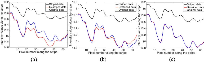
The next task is to check the accuracy of the estimated val-ues for the stripes. The stripe at the 110th row was randomly selected for this purpose. There we plot the intensity values of the stripe (black), reconstruction (red) and the actual val-ues as they were against the column index. The results from the functional in Eq. (3) withα=1 is shown in the graph (c) of Fig. 3. The reconstructions of the first 20 pixels and the last 10 pixels are closer to the original values, but the rest have significant differences compared to the actual value. The graph (b) in Fig. 3 shows destriped results of the 110th row from the functional in Eq. (3) using theU-curve solution,
α=3×10⁻¹. In this case, the reconstruction of some mid-dle pixels (18–28 and 31–37) and the last 10 pixels are off by some extent, but the rest is much closer to the actual values than the reconstruction withα=1. The graph (c) in Fig. 3 shows the best solution among these approaches, obtained from the weighted regularization term with α=7×10⁻¹. This reconstruction is very close to the actual values and hence it is the most accurate reconstruction. These are the sort of results that we expect from a destriping algorithm. More importantly, if we compare “a stripe-like feature” at the 18th row, we can confirm the importance of giving weights to the regularization term, as the weighted regularization term focus only the stripes.
func-Figure 3.This figure presents three different reconstructions of the stripe at the 110th row of the image shown in Fig. 1b. The graphs show the actual data in blue, striped data in black and the destriped data in red. Graphs(a)and(b)represent the reconstructions from the functional in Eq. (3) withα=1 andα=3×10⁻¹, respectively. The graph(c)shows the reconstruction from the functional in Eq. (6) withα=7×10⁻¹.
tional in Eq. (3) withα=1 andα=3×10⁻¹, respectively, and the graph (c) in Fig. 4 from the functional in Eq. (6) with
α=7×10⁻¹. The graphs (a) and (b) in Fig. 4 conclude that the destriping has affected the other features of the image when the functional in Eq. (3) is applied regardless of the value of the regularization parameter. However, the graph (c) in Fig. 4 shows that the functional with the spatially weighted regularization term in Eq. (6) does not affect the other fea-tures of the image.
TheScurve corresponding to the SST image is shown in graph (a) in Fig. 5. The “threshold” value for this problem is also shown on the same graph and it is 18 in this case. If we consider the units of the sea surface temperature data, the threshold value can written as 842◦C longitude per latitude. To determine the best “threshold” value that does not affect the image regions with no stripes, we begin the procedure by assigning the “threshold” value to the maximum peak of the
S curve. Then we apply the destriping algorithm and check the solution. If at least one stripe is still visible, we assign the next highest peak of theScurve as the “threshold” value and check for the stripes. Continuing in this manner until all the stripes are removed, the best “threshold” value can be determined. The peak points that have crossed the threshold value are the stripes. As a comparison of the full destriping image, the absolute percentage error between the striped and destriped image is shown in the image (b) in Fig. 5. This is computed by
Absolute Percentage Error=|f−u| f ×100,
wheref anduare striped and destriped images respectively. The graph of the absolute percentage error shows that not only the 67th row but also all the other non-stripe rows are not affected from this spatially weighted regularization method.
3.2 Example 2 – VIIRS images
A good example of VIIRS stripping is shown (Fig. 6) in a chlorophyll concentration map near the Santa Monica region in southern California on 7 November 2014 NAS (2014). The chlorophyll concentration is given in milligrams per cubic meter. Green is the land and the dark blue is the dropped data and the missing data. The full VIIRS data granule covers −122.09◦W to−116.90◦E and 34.2◦N to 31.6◦S (Fig. 6). We consider a subsetted (cropped) region of interest to high-light the stripes in Fig. 7a.
The first step of applying this destriping method is to de-termine the threshold value to separate the neighborhood of stripes and the rest of the features. However, when we deal with real data, we may not always get nice and smooth im-ages. For instance, if we compute theS curve values using the whole image, we are unable to get any evidence to de-termine the threshold value, as the sum of the magnitude of forward differences in some other rows are higher than that of the stripes. Therefore, we need to carefully pick a subregion of the image that includes all the rows with some selected columns. The sum of the magnitude of forward differences in non-stripe rows should be less than the that of stripes in this region. Then the stripes can be easily highlighted. For this example, we select the region using the columns from 137 to 148, and it is shown in Fig. 7b with theScurve. The threshold value can be determined from theS curve, and it is 0.558 for this image. If we include the proper units of the image data, the threshold value is 86.04 mg m−3.
The effects of spatially weighted regularizing destriping are shown in Fig. 7e. We apply our algorithm to the image shown in Fig. 7a. In this case, the regularization parameter wasα=10−2with the weighted regularization term. The in-tensity of the destriped image now varies smoothly. There-fore, the image is smooth enough to further post-process for other applications such as computing optical flow.
Figure 4.This figure shows the effects of destriping on the places where there are “no stripes”. We randomly picked the 67th row for this comparison. Whenα=1 in the unweighted regularization functional, the image is more smoothed and affects destriping to the whole image. Much better results can be obtained from the unweighted regularization functional withα=3×10⁻¹, which is theU-curve solution and is shown in graph(b). A spatially weighted regularization term withα=7×10⁻¹has less of an effect on the other features of the image and we can observe that from the graph(c).
Figure 5.Panel(a)shows theSfunction values against the column numbers. The peak points represent the stripes. When “threshold” is set at 18, only stripes can be included for the regularization but excludes all the other features of the image. With the units of the image data, the threshold value can written as 842◦C longitude per latitude. Then the percentage error between the striped and destriped image are shown in the panel(b). The error where there are no stripes is always closer to the zero.
our functional Eq. (3). However, our destriping functional as shown in Eq. (6) has weight matrixLinside the regulariza-tion term and hence the two approaches are not the same. Panel (c) in Fig. 7 represents the destriped image whenα=1 without the weighted regularization term, where image (a) is the original image. The destriped image is blurred and we lose some information from the original image due to “over regularization”. In this case, by over regularization we mean that continuity in the transverse direction to the “stripes” has been emphasized so strongly in functional Eq. (3), whenαis close to 1, that it is past balance against the need to also em-phasize the image data in the first term, called “data fidelity”.
Figure 6.The image shows the chlorophyll concentration in milligrams per cubic meter near the Santa Monica region in southern California as viewed by VIIRS on 7 November 2014. Green represents the land and dark blue represents the dropped data due to bow-tie effects and missing data due to clouds. For a detailed discussion, we next consider the subset of the image that is covered by the pink square in the image.
Figure 7.Panel(a)shows the cropped region shown in Fig. 6 and the graph(b)shows theScurve with the threshold and the image piece (columns 137 to 148) that we used compute the values ofS curve. The panels(c),(d)and(e)represent the destriped images of(a)with
Figure 8.Panel(a)shows the destriped image scene of the panel(a)in Fig. 7 from NASA’s vicarious calibration of The L2 (*.nc) product method. While NASA’s vicarious calibration of The L2 (*.nc) product method does improve over the raw image, there are still stripe artifacts present. The following image(b)represents the destriped image of the image(a)from our method.
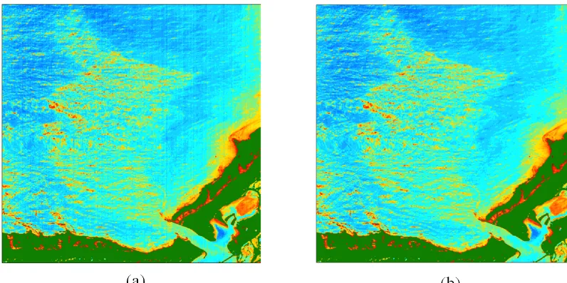
Figure 9.Panel(a)is band 22 (∼410 nm) of a hyperspectral image which was taken from JPL PRISM JPL (2015). The stripe pattern is vertical and the destriped images are shown in image(b). Green represents the land of the observed region.
selected from theU-curve method, as explained in Sect. 2.3. Panel (f) in Fig. 7 shows the percentage error between the striped and destriped images. This is proof that the effects from the destriping on the image where there are no stripes is negligible.
Image-based methods such as the variational destriping can be used together with other destriping methods. For in-stance, NASA’s vicarious calibration of the L2 (*.nc) product method uses a monthly moon calibration to monitor the strip-ing and calibrations and create up-to-date corrections usstrip-ing the entire image collection. Figure 8a shows the VIIRS im-age in Fig. 7a after the NASA correction, and the data are publicly available at NAS (2014). However, the striping arti-facts are still visible in that image. Fig. 8b shows the appli-cation of the weighted regularizing destriping to the image
from NASA’s vicarious calibration of The L2 (*.nc) prod-uct method. The prodprod-uct from the applications of both cor-rections is superior to either individual correction. The reg-ularization parameter for this image was 5×10⁻³, and the destriped image is shown in Fig. 8b. The threshold value for the columns 137 to 148 was 0.55. If we include the proper units of the chlorophyll data, the threshold value is 84.81 (mg) longitude/(m3) latitude.
3.3 Example 3 – JPL PRISM images
In the last example, we apply the variational destriping algo-rithm to another data set from the JPL PRISM hyperspectral imager, where the data is publicly available at JPL (2015). Stripes arise in this sensor because of the focal-plane array read-out mechanism has cross-talk artifacts. An image from the band centered at 410 nm (band 22), which was taken from an airborne campaign around Monterey, CA, near the Elkhorn Slough (Pantazis et al., 2015), is shown in Fig. 9.
The regularization parameter to destripe the image (a) in Fig. 9 wasα=5×10⁻³. The destriped image is shown in image (b) in Fig. 9. We used the columns from 50 to 70 to determine the threshold value to assign the weights in the regularization term, and this value was 1.7 for this image. It can be clearly observed that the stripes are smoothed from the destriping method while preserving the other features of the image.
4 Conclusions
We present a variational destriping method by explicitly in-cluding a tunable regularization parameter with a weighted regularization term to a part of the destriping functional in Bouali (2010). In other words, we modeled one piece of the destriping functional in Bouali (2010) into a standard variational-based approach employing the Tikhonov regular-ization theory of Vogel (2002). According to the Tikhonov regularization theory, the tuning parameter allows us to prop-erly balance the effects of optimizing the data fidelity and the smoothing effects of regularization term with the help of given weights. The introduction of the weighted regulariza-tion term avoids the effects on the original features of the image during the process of destriping. As a preprocessing step, we apply an image-processing technique to avoid the error accumulation from the “bow-tie” effects and missing data due to clouds. We also demonstrate alternative numeri-cal aspects to implementing these methods, which allows us to write the solver in terms of common matrix manipulations. Lastly, we show that applying a scene-based method to the destriped VIIRS L2 product from NASA calibration method results in additional improvements in scene uniformity.
Data availability. We used three data sets (SST, VIIRS and PRISM) in our paper. They are VIIRS data at https://oceancolor. gsfc.nasa.gov/ and PRISM data at https://prism.jpl.nasa.gov/. SST data are not publicly accessible. The data are available by a request to John Osborn, Oregon State University.
Author contributions. R. Basnayake, E. Bollt and J. Sun developed the variational-based destriping algorithm. N. Tufillaro collected raw data from reliable sources and processed the data so that it could
be readable in MATLAB. M. Gierach provided the JPL-PRISM data.
Competing interests. The authors declare that they have no conflict of interest.
Acknowledgements. The authors Ranil Basnayake, Erik Bollt, Nicholas Tufillaro and Jie Sun were supported by the Na-tional Geospatial Intelligence Agency under grant number HM02101310010. Erik Bollt was also supported by the Office of Naval Research, PI, N00014-15-1-2093, thanks to the Office of Naval Research grant no. N00014-16-1-2492.
Edited by: Stephen Wiggins
Reviewed by: Kevin McIlhany and one anonymous referee
References
Basnayake, R. and Bollt, E. M.: A Multi-time Step Method to Com-pute Optical Flow with Scientific Priors for Observations of a Fluidic System, in: Ergodic Theory, Open Dynamics, and Coher-ent Structures, Springer, 59–79, 2014.
Bertalmio, M., Sapiro, G., Caselles, V., and Ballester, C.: Image in-painting, in: Proceedings of the 27th annual conference on Com-puter graphics and interactive techniques, ACM Press/Addison-Wesley Publishing Co., 417–424, 2000.
Bertalmio, M., Caselles, V., Masnou, S., and Sapiro, G.: Inpainting, Encyclopedia of Computer Vision, 2011.
Bouali, M.: A simple and robust destriping algorithm for imaging spectrometers: Application to MODIS data, in: Proceedings of ASPRS 2010 Annual Conference, San Diego, CA, USA, vol. 2630, 84–93, 2010.
Bouali, M. and Ignatov, A.: Adaptive Reduction of Striping for Im-proved Sea Surface Temperature Imagery from Suomi National Polar-Orbiting Partnership (S-NPP) Visible Infrared Imaging Ra-diometer Suite (VIIRS), J. Atmos. Ocean. Tech., 31, 150–163, https://doi.org/10.1175/JTECH-D-13-00035.1, 2013.
Cao, C., Xiong, X., Wolfe, R., De Luccia, F., Liu, Q., Blonski, S., Lin, G., Nishihama, M., Pogorzala, D., Oudrari, H., and others: Visible Infrared Imaging Radiometer Suite (VIIRS) Sensor Data Record (SDR) User’s Guide. Version 1.2, 10 September 2013, NOAA Technical Report NESDIS, 142, 2013.
Eplee, R. E., Turpie, K. R., Fireman, G. F., Meister, G., Stone, T. C., Patt, F. S., Franz, B. A., Bailey, S. W., Robinson, W. D., and McClain, C. R.: VIIRS on-orbit calibration for ocean color data processing, vol. 8510 of Proc. SPIE, 85101G–85101G–18, 2012. Hansen, P. C.: Analysis of discrete ill-posed problems by means of
the L-curve, SIAM Rev., 34, 561–580, 1992.
Hansen, P. C.: The L-Curve and its Use in the Numerical Treat-ment of Inverse Problems, in: Computational Inverse Problems in Electrocardiology, Advances in Computational Bioengineer-ing, edited by: Johnston, P., WIT Press, 119–142, 2000. Hansen, P. C.: Discrete inverse problems: insight and algorithms,
Hansen, P. C., Nagy, J. G., and O’leary, D. P.: Deblurring images: matrices, spectra, and filtering, vol. 3, Siam, Society for Indus-trial and Applied Mathematics, 2006.
JPL: Portable Remote Imaging Spectrometer, available at: http:// prism.jpl.nasa.gov/prism_data.html, last access: 20 May 2015. Krawczyk-Stado, D. and Rudnicki, M.: The use of L-curve and
U-curve in inverse electromagnetic modelling, Stud. Comp. Intell., 119, 73–82, 2008.
Krawczyk-Sta´nDo, D. and Rudnicki, M.: Regularization parameter selection in discrete ill-posed problems—the use of the U-curve, Int. J. Appl. Math. Comp., 17, 157–164, 2007.
Mikelsons, K., Wang, M., Jiang, L., and Bouali, M.: Destriping al-gorithm for improved satellite-derived ocean color product im-agery, Opt. Express, 22, 28058–28070, 2014.
Mikelsons, K., Ignatov, A., Bouali, M., and Kihai, Y.: A fast and robust implementation of the adaptive destriping algorithm for SNPP VIIRS and Terra/Aqua MODIS SST, vol. 9459 of Proc. SPIE, 94590R–94590R–13, 2015.
NASA Ocean Color, available at: http://oceancolor.gsfc.nasa.gov/ cgi/browse.pl?sen=am, last access: 1 June 2014.
Osborne, J., Kurapov, A., Egbert, G., and Kosro, P.: Spatial and tem-poral variability of the M 2 internal tide generation and propa-gation on the Oregon shelf, J. Phys. Oceanogr., 41, 2037–2062, 2011.
Pantazis, M., Gorp, B. V., Dierseen, H., Blerach, M., and Fichot, C.: The Portable Remote Imaging Spectrometer (PRISM): Recent Campaigns and Developments, Fourier Transform Spectroscopy and Hyperspectral Imaging and Sounding of the Environment, HM4B.5, OSA, 2015.