Relative impact of model quality and ensemble deﬁciencies on the performance of ensemble based probabilistic forecasts evaluated through the Brier score

(1)

Nonlinear Processes in Geophysics (2004) 11: 399–409

SRef-ID: 1607-7946/npg/2004-11-399

Nonlinear Processes

in Geophysics

Relative impact of model quality and ensemble deficiencies on the

performance of ensemble based probabilistic forecasts evaluated

through the Brier score

F. Atger

Meteo-France (DPREVI), 42, av. G. Coriolis, 31057 Toulouse cedex, France

Received: 24 November 2003 – Revised: 30 June 2004 – Accepted: 24 July 2004 – Published: 14 September 2004

Abstract. The relative impact of model quality and ensemble deficiencies, on the performance of ensemble based proba-bilistic forecasts, is investigated from a set of idealized exper-iments. Data are generated according to a statistical model, the validation of which is achieved by comparing generated data to ECMWF ensemble forecasts and analyses. The per-formance of probabilistic forecasts is evaluated through the reliability and resolution terms of the Brier score. Results are as follows. (i) Resolution appears essentially attributable to the average level of forecast skill. (ii) The lack of reliabil-ity comes primarily from forecast bias, and to a lower extent from the ensemble being systematically under-dispersive (or over-dispersive). (iii) Forecast skill contributes very little to reliability in the absence of forecast bias, and this impact is entirely due to the finiteness of the ensemble population. (iv) In the presence of forecast bias, reducing forecast skill leads to improve the reliability. This unexpected feature comes from the fact that lower forecast skill leads to a larger en-semble spread, that compensates for the strong proportion of outliers consequent to forecast bias. (v) The lack of ensemble skill, i.e. non systematic errors affecting both ensemble mean and ensemble spread, contributes little, but significantly, to the lack of reliability and resolution.

1 Introduction

The validation of operational ensemble prediction systems (EPS) has become an important field of research during the past few years (e.g. Zhu et al., 2001 and references therein). Among other objectives, validation aims at pointing the ad-vantages and drawbacks of the scientific options that have been adopted for the different aspects of the development of an operational EPS: method for the selection of initial pertur-bations, number of ensemble members, choice of a “stochas-tic” physics vs. the multi-model approach, etc. Therefore, Correspondence to: F. Atger

([email protected])

validation often requires a comparison of the performance of ensembles run in meteorological centres where the research strategy differs significantly (e.g. Mullen and Buizza, 2001). This is the case for example when comparing the perfor-mance of the two operational ensembles that have been run since the early 1990’s, at the U.S. National Centers for En-vironmental Prediction (NCEP) (Tracton and Kalnay 1993), and at the European Centre for Medium-range Weather Fore-casts (ECMWF) (Palmer et al., 1993).

On the other hand, operational ensembles run by different centres are generally based on different forecasting systems, i.e. numerical models and assimilation systems (including the way available observations are collected and selected) that differ sufficiently for giving different forecasts in a given situation. The performance of these forecasting systems is likely to differ, so that the results of a comparison between two EPS may not reflect solely the differences related to the strategy that has been followed for designing the ensemble. The performance of the underlying forecasting system obvi-ously contributes to the overall performance of an ensemble. Normalization of the results allows to compensate for this effect to a certain extent, e.g. when computing a skill-score with respect to a control forecast (Atger, 1999). However, interpretation of such normalized results may be problematic if the relative impact of the quality of the forecasting system, compared to deficiencies intrinsically related to the way the EPS has been designed, remains unknown.

(2)

400 F. Atger: Relative impact of model quality and ensemble deficiencies

19/24

Figures

0 0.5 1 1.5

ensemble standard deviation 0 0.01 0.02 0.03 0.04 0.05 0.06 0.07 0.08 frequency

0 0.25 0.5 0.75 1 1.2 1.5 ensemble standard deviation

0 0.25 0.5 0.75 1 1.2 1.5

ensemble mean RMSE

Figure 1. Distribution of the +96-hour ECMWF ensemble standard deviation, sampled with 67 intervals

(solid line), fitted with a transformation of the form

)]

1

,

0

Ν

(

exp[

β

α

σ

=

with

α

=0.4 and

β

=0.5 (dashed

line).

Figure 2. Correspondence between the +96-hour ECMWF ensemble standard deviation (abcissa) and the

ensemble mean RMSE (ordinate). Data have been stratified into 61 classes according to the EPS standard deviation. The average standard deviation in each class

is plotted against the RMSE of the ensemble mean computed from the cases found in the class.

0 0.25 0.5 0.75 1 1.2 1.5

ensemble standard deviation 0 0.25 0.5 0.75 1 1.2 1.5

ensemble mean RMSE

0 0.25 0.5 0.75 1 1.2 1.5

ensemble standard deviation 0 0.25 0.5 0.75 1 1.2 1.5

ensemble mean RMSE

Figure 3. Same as Fig. 2, but from generated data (100000 cases). The generated ensemble is perfect with

respect to any other aspect than under-dispersion (fs=0.5, fb=-0.16, sb=0.9, sv=0.2, ems=0, ess=0).

Figure 4. Same as Fig. 3, but non systematic ensemble deficiencies are considered

(fs=0.5, fb=-0.16, sb=0.9, sv=0.2, ems=0.1, ess=0.5). Fig. 1. Distribution of the +96-hour ECMWF ensemble standard

deviation, sampled with 67 intervals (solid line), fitted with a trans-formation of the formσ=αexp[βN (0,1)]withα=0.4 andβ=0.5 (dashed line).

reliability indicates to which extent a given ensemble distri-bution proves close to the conditional pdf (probability den-sity function) of the future state of the atmosphere. An es-timate of the latter is given by the distribution of the atmo-spherical states that are observed when a given ensemble dis-tribution is forecast. The second attribute is the resolution, that quantifies the variability of the observed frequency of an event, when the forecast probability of this event varies. In a more general sense, resolution indicates the variability of the conditional pdf, sampled by the observations, when the ensemble distribution varies.

The primary goal of the work presented in this article is to determine to which extent the performance of ensemble based probabilistic forecasts is conditioned by the quality of the underlying forecasting system, i.e. the atmospheric model and the assimilation system. The impact of certain as-pects of the quality of an EPS, that are assumed independent of the quality of the forecasting system, is investigated too. Idealized experiments have been designed in order to evalu-ate the impact of these different factors. The performance of probabilistic forecasts is quantified through the computation of the reliability and resolution terms of the Brier score.

The article is organized as follows. The methodology is exposed in Sect. 2. Results are exposed in Sect. 3, discussed in Sect. 4, summarized in Sect. 5.

2 Data and methodology 2.1 Data

Data for the idealized experiments have been generated ac-cording to a statistical model described in Sect. 2.3. The rel-evance of this statistical model has been tested by comparing the generated data to analyses and forecasts extracted from the ECMWF archive. Ensemble forecasts and analyses of the

19/24

Figures

0 0.5 1 1.5

0 0.25 0.5 0.75 1 1.2 1.5

ensemble mean RMSE

)]

1

,

0

Ν

(

exp[

β

α

σ

=

with

α

=0.4 and

β

=0.5 (dashed

line).

0 0.25 0.5 0.75 1 1.2 1.5

ensemble mean RMSE

0 0.25 0.5 0.75 1 1.2 1.5

ensemble mean RMSE

(fs=0.5, fb=-0.16, sb=0.9, sv=0.2, ems=0.1, ess=0.5). Fig. 2. Correspondence between the +96-hour ECMWF ensemble standard deviation (abcissa) and the ensemble mean RMSE (ordi-nate). Data have been stratified into 61 classes according to the EPS standard deviation. The average standard deviation in each class is plotted against the RMSE of the ensemble mean computed from the cases found in the class.

850-hPa temperature anomaly at 48 grid points over Europe (35◦)N, 60◦)N, 10◦)W, 25◦)E, 5×5◦)have been retrieved for a period of 4 consecutive winter seasons (December to February), from 10 December 1996 to 28 February 2000, i.e. 351 days. Sample size is 351×48=16 848 cases, considered in this idealized study as independent realizations of a unique random variable. During the considered period the opera-tional version of the ECMWF EPS has been improved several times, as well as the atmospheric model on which it is based, but the horizontal resolution remained the same (TL159), as

well as the number of ensemble members (N=50 perturbed integrations + 1 control integration). Analyses come from the ECMWF high resolution model that was operational during the same period (TL319). The climate reference, for the

def-inition of anomalies, has been computed from the ECMWF 15-year reanalysis (Gibson et al. 1997). All data have been standardized with respect to the local analysis standard devi-ation.

2.2 Verification

The performance of ensemble based probabilistic forecasts has been estimated through reliability diagrams and the com-putation of the Brier score. Unless otherwise stated, the con-sidered event is a positive deviation above 1 standard devia-tion from the origin.

(3)

F. Atger: Relative impact of model quality and ensemble deficiencies 401

19/24

Figures

0 0.5 1 1.5

0 0.25 0.5 0.75 1 1.2 1.5

ensemble mean RMSE

)]

1

,

0

Ν

(

exp[

β

α

σ

=

with

α

=0.4 and

β

=0.5 (dashed

line).

0 0.25 0.5 0.75 1 1.2 1.5

ensemble mean RMSE

0 0.25 0.5 0.75 1 1.2 1.5

ensemble mean RMSE

(fs=0.5, fb=-0.16, sb=0.9, sv=0.2, ems=0.1, ess=0.5). Fig. 3. Same as Fig. 2, but from generated data (10 0000 cases). T

he generated ensemble is perfect with respect to any other aspect than under-dispersion (fs=0.5, fb=-0.16, sb=0.9, sv=0.2, ems=0,

ess=0).

The Brier score (BS) is defined for a dichotomous event as the mean square error of the probability forecast:

BS=1 M

M

X

i=1

(pi−oi)2, (1)

whereMis the number of cases,pi is the forecast

probabil-ity,oi is the verifying observation (oi=1 if the event occurs,

oi=0 if it does not) (Brier 1950). The Brier score is

tradition-ally transformed into a decomposition of 3 terms, inititradition-ally proposed by Murphy (1973):

BS=

T

X

k=1

mk

M(pk−ok)

2₋ T

X

k=1

mk

M(ok−o)

2₊_o(₁₋_o),₍₂₎

when the sample has been divided intoT categories, each comprisingmkcases when the probabilitypk is forecast.ok

is the observed frequency of the considered event whenpkis

forecast.ois the observed frequency in the whole sample. The first part of the decomposition is the reliability term, i.e. the integration, over the whole range of forecast probabil-ities, of the square difference between the probability and the observed frequency of the event. The reliability term of the Brier score can be seen graphically as the weighted, squared distance between the reliability curve and the 45◦line. It in-dicates to which extent the forecast probability is calibrated with respect to the a posteriori observed frequency of the considered event.

The second part of the decomposition is the resolution term, i.e. the variance, over the range of forecast proba-bilities, of the observed frequency of the event. The res-olution term of the Brier score can be seen graphically as the weighted, squared distance between the reliability curve

19/24

Figures

0 0.5 1 1.5

0 0.25 0.5 0.75 1 1.2 1.5

ensemble mean RMSE

)]

1

,

0

Ν

(

exp[

β

α

σ

=

with

α

=0.4 and

β

=0.5 (dashed

line).

0 0.25 0.5 0.75 1 1.2 1.5

ensemble mean RMSE

0 0.25 0.5 0.75 1 1.2 1.5

ensemble mean RMSE

(fs=0.5, fb=-0.16, sb=0.9, sv=0.2, ems=0.1, ess=0.5). Fig. 4. Same as Fig. 3, but non systematic ensemble deficiencies are considered (fs=0.5, fb=-0.16, sb=0.9, sv=0.2, ems=0.1, ess=0.5).

and the horizontal line indicating the sample frequency of the considered event. It indicates to which extent the fore-cast probability discriminates between occurence and non-occurence of the considered event.

The third part of the decomposition is the uncertainty term, i.e. the variance of the observations, that does not depend on the forecast system but rather reflects the intrinsic difficulty in forecasting the observations.

The resolution term is bounded by the uncertainty term, so that it is convenient to compute the standardized resolution as the ratio of the 2 terms, i.e._o(11₋_o)

T

P

k=1 mk

M(ok−o)

2_{. This ratio}

takes its maximum value (Eq. 1) in the case of a perfect deter-ministic forecast, and more generally when only two proba-bility categories are forecast, leading to observed frequencies 0 and 1. On the other hand the resolution term equals 0 when the observed frequency of the event is the same whatever the forecast probability.

Note that the reliability term is negatively oriented, as the Brier score (the lower the better) while the resolution term is positively oriented.

2.3 Statistical model

2.3.1 Assumptions and definitions

(4)

20/24

0 0.2 0.4 0.6 0.8 1

forecast probability 0

0.2 0.4 0.6 0.8 1

observed frequency

0 0.2 0.4 0.6

0 0.2 0.4 0.6 0.8 1

0.2 0.4 0.6 0.8 1

observed frequency

0 0.2 0.4 0.6

(a) (b)

0 0.2 0.4 0.6 0.8 1

0.2 0.4 0.6 0.8 1

observed frequency

0 0.2 0.4 0.6

0 0.2 0.4 0.6 0.8 1

0.2 0.4 0.6 0.8 1

observed frequency

0 0.2 0.4 0.6

(c) (d)

0 0.2 0.4 0.6 0.8 1

0.2 0.4 0.6 0.8 1

observed frequency

0 0.2 0.4 0.6

0 0.2 0.4 0.6 0.8 1

0.2 0.4 0.6 0.8 1

observed frequency

0 0.2 0.4 0.6

(e) (f)

(5)

F. Atger: Relative impact of model quality and ensemble deficiencies 403 forecast bias of ensemble members is thus identical to that

of the reference run (i.e. the integration from the reference initial state). Ensemble members are normally distributed. Unless otherwise stated, the number of ensemble members is fixed to 51 (in order to facilitate comparisons to the ECMWF ensemble).

2.3.2 Perfect ensemble

In this section the forecasting system is assumed not to be bi-ased, i.e. the mean error of the reference run is zero, as well as that of any ensemble member. The perfect ensemble is defined as an idealized, perfectly reliable ensemble, whose members are assumed to be drawn fromN(mp,sp),

accord-ing to the normal assumption mentioned above. Since there is no forecast bias, the perfect ensemble meanmpis a draw

from the truth distribution, i.e.N(0, 1). The perfect ensemble standard deviationsp is arbitrarily drawn fromαexp[βN(0,

1)] (log-normal distribution). Figure 1 shows that this choice is consistent with the actual distribution of the standard devi-ation of the ECMWF operdevi-ational ensemble.

Since the perfect ensemble is perfectly reliable, the ver-ifying observation is also drawn fromN(mp,sp). The

stan-dard deviation of this distribution indicates the level of uncer-tainty related to the forecast of the verifying observation (the ensemble being perfect, this uncertainty is indeed perfectly related to the ensemble spread). Therefore, the mean ofsp

indicates the average level of forecast uncertainty, given the forecasting system under consideration, called forecast skill (fs) in the following. Similarly, the standard deviation ofsp

indicates the variability of the level of forecast uncertainty, called skill variability (sv) in the following. The parame-ters fs and sv indicate two characteristics of the forecasting system that are independent of other parameters that might characterize the way an ensemble is designed.

From the above definitions, it comes thatα = √ f s2

f s2₊_sv2 andβ2=log(sv2

f s2 +1).

The average level of forecast skill (fs), as well as the vari-ability of the forecast skill (sv), are related to the level of atmospheric predictability. However, in the present study, predictability is not seen as an intrinsic property of the atmo-sphere, but rather reflects the ability of a given forecasting system to predict the evolution of the atmosphere. Although it is obviously constrained by the actual initial conditions, forecast skill is thus an attribute of the quality of a forecast-ing system. And its variability, highly dependent on the at-mosphere dynamics, is still a characteristic of the forecasting system.Generated ensembles Imperfect ensembles are gener-ated from a (potentially) biased forecasting system. Specifi-cally, ensemble members are drawn from a normal distribu-tion N(me,se)that differs fromN(mp,sp)according to

sys-tematic deficiencies of both the forecasting system and the ensemble. First, a systematic forecast bias (fb) is taken into account:

me =mp+f b. (3)

21/24

0 0.2 0.4 0.6 0.8 1

0.2 0.4 0.6 0.8 1

observed frequency

0 0.2 0.4 0.6

(g)

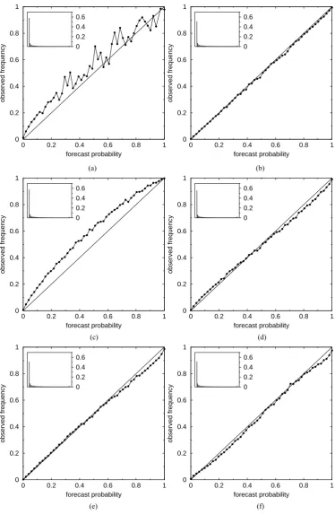
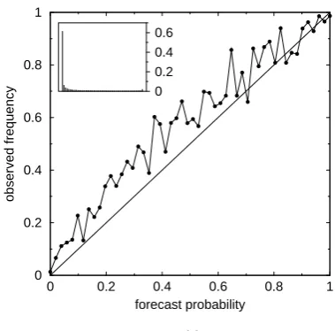
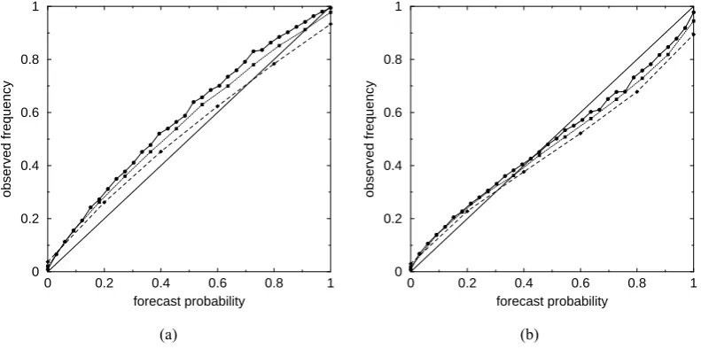
Figure 5. Reliability diagrams. The main curve indicates the correspondence between a given forecast probability (abcissa) and the observed frequency of the event when this probability is forecast (ordinate). The histogram shows the distribution of forecast probabilities. The event is a positive deviation of 1 standard deviation from the origin. (a) Probability based on +96-hour ECMWF ensemble forecasts (16848 cases). (b) to (f) Probability based on generated data (1 million cases). Forecast skill is set to fs=0.5, skill variability is set to sv=0.2. (b) No forecast bias, perfect ensemble (no spread bias, ems=ess=0). (c) Effect of forecast bias: fb=-0.16, perfect ensemble. (d) Effect of spread bias: no forecast bias, sb=0.9, perfect ensemble otherwise (ems=ess=0). (e) Effect of a strong lack of ensemble mean skill: no forecast bias, no spread bias, ems=0.2, ess=0. (f) Effect of a strong lack of ensemble spread skill: no forecast bias, no spread bias, ems=0, ess=0.6. (g) Same as (b) to (f) but based on 16848

cases only, and with an arbitrary set of parameters: fb=-0.16, sb=0.9, ems=0.1, ess=0.5.

Fig. 5. Continued.

Secondly, a systematic (negative) spread bias (sb), i.e. a sys-tematic under-dispersion, is taken into account (0<sb<1 for the sake of realism, but with no loss of generality):

se=spsb. (4)

The parameter fb is a characteristic of the forecasting sys-tem that is independent on the way the ensemble is designed (under the assumptions given in Sect. 2.3.1), while sb is a characteristic of the ensemble that has no reason to depend on the quality of the forecasting system.

At this stage, the generated ensemble is perfect with re-spect to any other are-spect of the performance than the system-atic lack of dispersion. As a consequence the relationship be-tween ensemble spread and forecast skill is virtually perfect, although systematically biased when sb<1 (Fig. 3). This is clearly not a realistic feature when compared to an opera-tional ensemble as the ECMWF EPS (Fig. 2). Non system-atic aspects of the “intrinsic” quality of the generated ensem-ble (i.e. independent on the quality of the underlying fore-casting system) are taken into account by modifying Eqs. (3) and (4):

me=ξm(mp+f b) (30)

se=ξsspsb, (40)

whereξmandξs are drawn from a uniform distribution

cen-tered in 1. The half-amplitude of the distribution ofξm(ξs)

(6)

22/24

0.1 0.3 0.5 0.7 0.9

forecast skill

0

0.002

0.004

0.006

0.008

0.01

0

0.1

0.2

forecast bias

0

0.1

0.2

forecast skill variability

0.6 0.7 0.8 0.9

spread bias

0

0.1

0.2

ensemble mean skill

0

0.002

0.004

0.006

0.008

0.01

0 0.2 0.4 0.6 0.8

ensemble spread skill

Figure 6. Reliability term of the Brier score as a function of the different factors. The forecast skill is arbitrarily

set to

fs

=0.5, except when it varies. The skill variability is arbitrarily set to

sv

=0.2, except when it varies. The

impact of forecast skill is evaluated in the case of a perfect ensemble (

sb

=1,

ems

=

ess

=0), with no forecast bias

(

fb

=0, solid curve) or in the case of a moderate negative forecast bias (

fb

=-0.16, dashed curve). The impact of

forecast bias is evaluated in the case of a perfect ensemble (

sb

=1,

ems

=

ess

=0). The impact of skill variability is

evaluated in the absence of forecast bias (

fb

=0) and with a perfect ensemble (

sb

=1,

ems

=

ess

=0). The impact of

spread bias is evaluated in the absence of forecast bias (

fb

=0) and with a perfect ensemble skill (

ems

=

ess

=0). The

impact of ensemble mean skill and ensemble spread skill is evaluated separately in the absence of forecast bias

(

fb

=0) and with no spread bias (

sb

=1).

0.1 0.3 0.5 0.7 0.9

forecast skill

0

0.2

0.4

0.6

0.8

1

0

0.1

0.2

forecast bias

0

0.1

0.2

0.6 0.7 0.8 0.9

spread bias

0

0.1

0.2

ensemble mean skill

0

0.2

0.4

0.6

0.8

1

0 0.2 0.4 0.6 0.8

Figure 7. Same as Fig. 6, but for the resolution term of the Brier score. The effect of a negative forecast bias on

the impact of the forecast skill is not shown (undistinguishable).

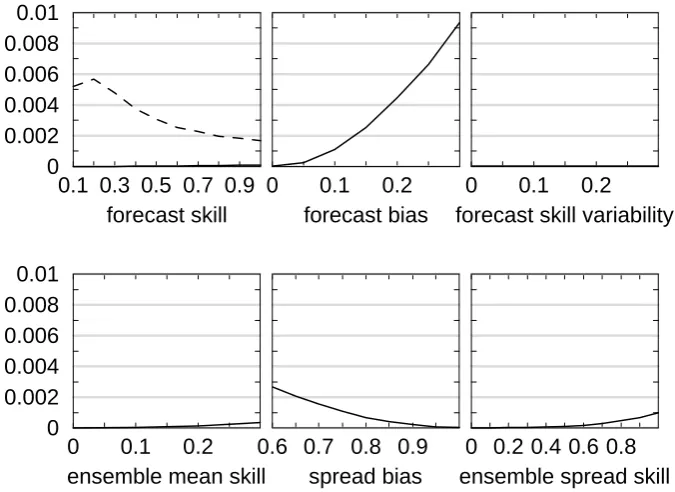
Fig. 6. Reliability term of the Brier score as a function of the different factors. The forecast skill is arbitrarily set to fs=0.5, except when it varies. The skill variability is arbitrarily set to sv=0.2, except when it varies. The impact of forecast skill is evaluated in the case of a perfect ensemble (sb=1, ems=ess=0), with no forecast bias (fb=0, solid curve) or in the case of a moderate negative forecast bias (fb=−0.16, dashed curve). The impact of forecast bias is evaluated in the case of a perfect ensemble (sb=1, ems=ess=0). The impact of skill variability is evaluated in the absence of forecast bias (fb=0) and with a perfect ensemble (sb=1, ems=ess=0). The impact of spread bias is evaluated in the absence of forecast bias (fb=0) and with a perfect ensemble skill (ems=ess=0). The impact of ensemble mean skill and ensemble spread skill is evaluated separately in the absence of forecast bias (fb=0) and with no spread bias (sb=1).

2.4 Experiments

6 parameters determine the statistical model that has been used for running the experiments. The 3 parameters fb (fore-cast bias), fs (fore(fore-cast skill) and sv (skill variability) indicate the quality of the underlying forecasting system. They are independent of the characteristics of the generated ensemble. The parameters sb (spread bias), ems (ensemble mean skill) and ess (ensemble spread skill) are related to the intrinsic quality of the ensemble, since they are not attributable to the underlying forecasting system.

The method for generating the data, as described above, implies that the modification of certain parameters (fs and sv) have an impact on the distribution of observations. In order to get comparable results, all generated data have been stan-dardized with respect to the standard deviation of the gener-ated observations.

ECMWF ensemble forecasts at different lead-times have been compared to generated data in order to determine a re-alistic range for the different parameters.

The definition of the parameter fb allows a direct estima-tion, as the algebraic mean of the forecast error. Typical values are−0.1/−0.2 for +48/+144-hour ECMWF forecasts (−0.16 for +96-hour).

The parameter fs is assumed to be of the same order as the standard deviation of the forecast error of the EPS

con-trol forecast, therefore varying mainly according to the fore-cast lead-time. Typical values of the error are 0.3/0.7 for +48/+144-hour ECMWF forecasts (0.5 for +96-hour).

Skill variability (parameter sv) is assumed not to be very different from the day-to-day variability of the operational ensemble standard deviation. Typical values of spread vari-ability are 0.1/0.2 for +48/+144-hour ECMWF forecasts.

There is empirical evidence indicating that sb is moder-ately negative in operational ensembles, i.e. ensembles gen-erally suffer from a limited under-dispersion (e.g. Buizza, 1997; Toth and Kalnay, 1997).

Parameters ems and ess have been tuned empirically in or-der to reproduce the characteristics of operational ensembles, in particular the shape of the reliability curve and the rela-tionship between ensemble spread and forecast skill, when other parameters vary.

(7)

22/24

0.1 0.3 0.5 0.7 0.9

forecast skill

0

0.002

0.004

0.006

0.008

0.01

0

0.1

0.2

forecast bias

0

0.1

0.2

0.6 0.7 0.8 0.9

spread bias

0

0.1

0.2

ensemble mean skill

0

0.002

0.004

0.006

0.008

0.01

0 0.2 0.4 0.6 0.8

Figure 6. Reliability term of the Brier score as a function of the different factors. The forecast skill is arbitrarily

set to

fs

=0.5, except when it varies. The skill variability is arbitrarily set to

sv

=0.2, except when it varies. The

impact of forecast skill is evaluated in the case of a perfect ensemble (

sb

=1,

ems

=

ess

=0), with no forecast bias

(

fb

=0, solid curve) or in the case of a moderate negative forecast bias (

fb

=-0.16, dashed curve). The impact of

forecast bias is evaluated in the case of a perfect ensemble (

sb

=1,

ems

=

ess

=0). The impact of skill variability is

evaluated in the absence of forecast bias (

fb

=0) and with a perfect ensemble (

sb

=1,

ems

=

ess

=0). The impact of

spread bias is evaluated in the absence of forecast bias (

fb

=0) and with a perfect ensemble skill (

ems

=

ess

=0). The

impact of ensemble mean skill and ensemble spread skill is evaluated separately in the absence of forecast bias

(

fb

=0) and with no spread bias (

sb

=1).

0.1 0.3 0.5 0.7 0.9

forecast skill

0

0.2

0.4

0.6

0.8

1

0

0.1

0.2

forecast bias

0

0.1

0.2

0.6 0.7 0.8 0.9

spread bias

0

0.1

0.2

ensemble mean skill

0

0.2

0.4

0.6

0.8

1

0 0.2 0.4 0.6 0.8

Figure 7. Same as Fig. 6, but for the resolution term of the Brier score. The effect of a negative forecast bias on

the impact of the forecast skill is not shown (undistinguishable).

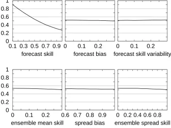
Fig. 7. Same as Fig. 6, but for the resolution term of the Brier score. The effect of a negative forecast bias on the impact of the forecast skill is not shown (undistinguishable).

the ensemble spread, other than the systematic lack of dis-persion) to 1 (large, non systematic errors affecting the en-semble spread).

3 Results

Unless otherwise stated, one million verification cases have been generated for each experiment. The impact of the dif-ferent factors is investigated by varying the value of the 6 parameters and evaluating the performance of probabilistic forecasts through reliability curves and the reliability and res-olution terms of the Brier score. Qualitatively, forecast skill and skill variability are expected to have an impact on res-olution. Forecast bias and spread bias are expected to have an impact on reliability. Ensemble mean skill and ensemble spread skill are expected to have an impact both on reliability and resolution.

3.1 Reliability curves

Figure 5 shows the reliability curve obtained from +96-hour ECMWF ensemble forecasts, as a reference (Fig. 5a), to-gether with those obtained with generated data. Forecast skill and skill variability have been arbitrarily fixed (fs=0.5, sv=0.2), since these two parameters are not expected to have any impact on reliability. The other parameters have been set as follows:

(i) No forecast bias (fb=0) and perfect ensemble, i.e. sb=1 and ems=ess=0 (Fig. 5b). Reliability is not perfect, although the observation is drawn from the same distribution as

en-semble members. Lower probabilities are slightly underesti-mated (this effect is hardly visible) while higher probabilities are slightly overestimated. The significance of this feature is discussed in Sect. 4.

(ii) Realistic forecast bias (fb=−0.16) and perfect ensem-ble (Fig. 5c). The typical effect of a negative bias is similar to that observed for ECMWF data (Fig. 5a). Because the sign of the bias is opposite to that of the considered event (pos-itive deviation larger than 1 standard deviation) the forecast probability is systematically underestimated.

(iii) No forecast bias, realistic spread bias (sb=0.9), per-fect ensemble otherwise i.e. ems=ess=0 (Fig. 5d). The efper-fect of spread bias is typical too: because of the systematic un-derdispersion, lower probabilities are underestimated while higher probabilities are overestimated. Combined to that of a negative forecast bias (Fig. 5c) this effect leads to a reliability curve close to that obtained from ECMWF data (Fig. 5a).

(iv) No forecast bias, no spread bias, but a strong lack of skill affects the ensemble mean only (ems=0.2, ess=0) (Fig. 5e). The impact is similar to that of a moderate spread bias: underestimation of lower probabilities, overestimation of higher probabilities.

(v) No forecast bias, no spread bias, but a strong lack of skill affects the ensemble spread only (ems=0, ess=0.6) (Fig. 5f). The typical impact is an overall overestimation of forecast probabilities, of the same amplitude as caused by a moderate spread bias.

(8)

406 F. Atger: Relative impact of model quality and ensemble deficiencies shown in Sect. 2.3.3 (Fig. 4) the parameters have been set

empirically as follows: fs=0.5, fb=−0.16, sv=0.2, sb=0.9, ems=0.1, ess=0.5. In order to get a similar level of “noise”, when plotting the reliability curve, as obtained from ECMWF data, the experiment consists here in generating 16848 cases only.

3.2 Reliability

Figure 6 shows the impact of the different factors, consid-ered separately, on the reliability term of the Brier score. The lack of reliability comes mainly from the forecast bias, and to a lower extent from the spread bias. The lack of ensem-ble skill, attributaensem-ble to non systematic errors affecting both the ensemble mean and the ensemble spread, has a limited impact. There is no impact of the forecast skill variability, as expected. In the absence of forecast bias the impact of forecast skill is very small, as expected, but reliability does improve slightly when the skill increases. This result is dis-cussed in Sect. 4.

When the forecast bias is set to fb=−0.16, reliability im-proves when the skill decreases, i.e. the reliability term of the Brier score is numerically reduced. This improvement is larger when the parameters fs and fb are comparable, i.e. when forecast bias and forecast error have the same ampli-tude, and it is emphasized when the forecast bias increases (not shown). This rather unexpected feature can be explained by the fact that increasing the forecast skill has the primary effect of decreasing the ensemble spread, provided the rela-tionship between spread and skill exists. When the forecast skill is high, the spread tends to be small and the ensemble distribution is sharp. The shift of the ensemble distribution with respect to the verification, attributable to the forecast bias, leads to a strong proportion of outliers. This induces a systematic underestimation of the forecast probability of an infrequent event (such as the event considered in the present study). When the forecast skill is lower, the spread tends to be large and the ensemble distribution is flatter. The propor-tion of outliers due to the forecast bias (i.e. related to the shift of the distribution) is thus reduced, so that the underestima-tion of the forecast probability is limited.

3.3 Resolution

Figure 7 shows the impact of the different factors on the reso-lution term of the Brier score, after standardization by the un-certainty term (Sect. 2.2). The main result is that resolution is almost entirely due to the forecast skill. Ensemble skill (pa-rameters ems and ess) has a definite impact, although small in amplitude. Resolution does increase with the skill variabil-ity, but the impact is hardly visible. On the other hand there is a slight decrease of resolution when the forecast bias or the spread bias grows. This last effect is discussed in Sect. 4.

23/24

0.1 0.3 0.5 0.7 0.9

forecast skill

10

−5

10

−4

10

−3

10

−2

Figure 8. Same as Fig. 6 (forecast skill panel only, y-coordinate follows a logarithmic scale), but the curves have been obtained by generating 10000 cases (solid line) and 1 million cases (dashed line).

0 0.2 0.4 0.6 0.8 1 forecast probability

0 0.2 0.4 0.6 0.8 1

observed frequency

0 0.2 0.4 0.6

0 0.2 0.4 0.6 0.8 1 forecast probability

0 0.2 0.4 0.6 0.8 1

observed frequency

Figure 9. Same as Fig. 5 (panel b) but computed from 10000 generated cases instead of 1 million.

Figure 10. Same as Fig. 5 (panel b) but the number of ensemble members is set to 33 (solid line, circles), 11 (dotted line, squares) and 5 (dashed line, diamonds). The distribution of forecast probabilities is not shown.

0.1 0.3 0.5 0.7 0.9

forecast skill

0

0.001

0.002

0.003

0.004

0.1

0.2

forecast bias

.6 0.7 0.8 0.9

spread bias

Figure 11. Same as Fig. 6 (forecast skill, forecast bias and spread bias panels only), but generated ensembles consisting of 11 members (dashed line) and 51 members

(solid line).

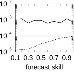
Fig. 8. Same as Fig. 6 (forecast skill panel only, y-coordinate fol-lows a logarithmic scale), but the curves have been obtained by gen-erating 10 000 cases (solid line) and 1 million cases (dashed line).

4 Discussion

4.1 Impact of the number of generated cases

The results presented in the previous section have been ob-tained by generating a very large number of cases for each experiment (one million). In the real world the number of verification cases that can be considered as independent real-izations of the same random variable is rather limited, espe-cially if one wants to take into account space and time cor-relations (Atger, 2003). A critical issue is thus whether the results presented above have any chance to be confirmed by performance evaluations based on real EPS data.

The relative impact of the different factors has been inves-tigated from 10 000 verification cases instead of 1 million. Variations of the reliability term of the Brier score are re-duced when the number of cases decreases. In particular, the slight degradation of reliability when the forecast skill decreases (in the absence of forecast bias) cannot be demon-strated with a sample consisting of 10 000 cases (Fig. 8). This seems to be due to the fact that this degradation is so tiny that it tends to be of the same order as the noise due to the lack of sampling.

(9)

23/24

0.1 0.3 0.5 0.7 0.9 forecast skill 0−5

0−4 0−3 0−2

0 0.2 0.4 0.6 0.8 1

0.2 0.4 0.6 0.8 1

observed frequency

0 0.2 0.4 0.6

0 0.2 0.4 0.6 0.8 1

0.2 0.4 0.6 0.8 1

observed frequency

0.1 0.3 0.5 0.7 0.9 forecast skill 0

0.001 0.002 0.003 0.004

0.1 0.2 forecast bias

.6 0.7 0.8 0.9 spread bias

(solid line).

Fig. 9. Same as Fig. 5b but computed from 10 000 generated cases instead of 1 million.

from 16 848 ECMWF cases accumulated over 4 winter sea-sons over Europe.

On the contrary, little effect has been found when reducing the size of the sample for evaluating the resolution term of the Brier score. Estimating resolution seems much easier, even from limited samples, than estimating reliability. This can be explained again by graphical considerations, the 45◦ line being generally closer to the reliability curve (due to the high level of reliability) than the horizontal line indicating the sample frequency of the event (Atger, 2004).

4.2 Impact of the number of ensemble members

For facilitating comparisons with the ECMWF operational EPS, the number of members of the generated ensembles has been set to N=51 in the previous section. Increasing or decreasingN may have an effect on the performance of ensemble based probabilistic forecasts, and consequently on the relative impact of the different factors that have been con-sidered.

Richardson (2001) has shown that decreasing the ensem-ble population results in a numerical increase of the relia-bility term of the Brier score, at least when the number of verification cases is large. It was mentioned in the previ-ous section how the lack of resolution makes the reliability curve pivot around the point indicating the correspondence between the average forecast probability and the overall fre-quency of the event, thus increasing the reliability term. Fig-ure 10 shows that this slope effect is emphasized whenN is reduced, leading to an increasing overestimation of probabil-ities above the frequency of the event. This can be seen as an effect of a poorer sampling of the pdf, due to the reduc-tion of the ensemble populareduc-tion. For example, when all the members forecast the event, the probability for the event to occur should not be 1 but “more thanN−1/N” since there is no way to estimate a probability betweenN−1/N and 1. In

23/24

0.1 0.3 0.5 0.7 0.9 forecast skill 0−5

0−4 0−3 0−2

0 0.2 0.4 0.6 0.8 1

0.2 0.4 0.6 0.8 1

observed frequency

0 0.2 0.4 0.6

0 0.2 0.4 0.6 0.8 1

0.2 0.4 0.6 0.8 1

observed frequency

0.1 0.3 0.5 0.7 0.9 forecast skill 0

0.001 0.002 0.003 0.004

0.1 0.2 forecast bias

.6 0.7 0.8 0.9 spread bias

(solid line).

Fig. 10. Same as Fig. 5b but the number of ensemble members is set to 33 (solid line, circles), 11 (dotted line, squares) and 5 (dashed line, diamonds). The distribution of forecast probabilities is not shown.

other words, whenN is small, extra ensemble members are missing that could sample the tails of the pdf. Similarly, ex-tra members are missing that could sample the pdf between 2 consecutive existing members.

In fact, one would expect the reliability term of the Brier score to be zero and the reliability curve to be perfectly aligned along the 45◦_{line in the case of a perfect ensemble.} If it is not exactly the case in Fig. 5b, and not at all the case in Fig. 10, it is just becauseN is finite. This effect is empha-sized when the forecast skill decreases (Fig. 11, forecast skill panel): because the uncertainty becomes larger, the number of members that are needed for sampling the pdf increases. When the error is low, even small (perfect) ensembles are able to sample the pdf, while a large number of (perfect) en-semble members is required when the error is high. Because the number of ensemble members is finite, only when the res-olution is perfect, i.e. when fs=0, the reliability term of the Brier score is zero in the case of a perfect ensemble (Figs. 6 and 11, forecast skill panel).

(10)

23/24

0.1 0.3 0.5 0.7 0.9

forecast skill

0

−5

0

−4

0

−3

0

−2

0 0.2 0.4 0.6 0.8 1

0.2 0.4 0.6 0.8 1

observed frequency

0 0.2 0.4 0.6

0 0.2 0.4 0.6 0.8 1

0.2 0.4 0.6 0.8 1

observed frequency

0.1 0.3 0.5 0.7 0.9

forecast skill

0

0.001

0.002

0.003

0.004

0.1

0.2

forecast bias

.6 0.7 0.8 0.9

spread bias

(solid line).

Fig. 11. Same as Fig. 6 (forecast skill, forecast bias and spread bias panels only), but generated ensembles consisting of 11 members (dashed line) and 51 members (solid line).

24/24

0 0.2 0.4 0.6 0.8 1

0.2 0.4 0.6 0.8 1

observed frequency

0 0.2 0.4 0.6 0.8 1

0.2 0.4 0.6 0.8 1

observed frequency

(a) (b)

Figure 12. Same as Fig. 5, panels (c) and (d) respectively, but the number of ensemble members is set to 33 (solid line, circles), 11 (dotted line, squares) and 5 (dashed line, diamonds). The distribution of forecast

probabilities is not shown.

Fig. 12. Same as Figs. 5c and d, respectively, but the number of ensemble members is set to 33 (solid line, circles), 11 (dotted line, squares) and 5 (dashed line, diamonds). The distribution of forecast probabilities is not shown.

An increase of the spread bias also tends to attenuate the impact on reliability of a reduction of the number of ensem-ble members (Fig. 11, spread bias panel). Only in the case of a strong spread bias the reliability term of the Brier score increases with the number of ensemble members. Again, this is because the effect of underdispersion compensates that of reducing the number of ensemble members (Fig. 12b). The former leads to an underestimation of forecast probabilities, for an infrequent event, while the latter leads to an overesti-mation of probabilities above the frequency of the considered event.

Decreasing the ensemble population has only little (nega-tive) effect on resolution. The relative impact of the different factors is unchanged, i.e. the forecast skill explains almost all the variations of the resolution term of the Brier score.

The combined effect of limiting both the number of en-semble members and the number of verification cases is be-yond the scope of this paper. This is a crucial issue for the validation of operational ensembles that has been extensively studied by Candille (2003a, b).

4.3 Impact of the frequency of the forecast event

All the results presented above have been obtained for an event occurring with an overall frequency close to 16% (pos-itive deviation above 1 standard deviation). Considering less frequent events (e.g. a positive deviation above 2 standard deviations) has the effect of decreasing the reliability term of the Brier score, especially when the forecast bias and/or the spread bias is high (not shown). However, the relative impact of the different factors is roughly unchanged, except that forecast bias and spread bias contribute at a closer level to the reliability term of the Brier score (not shown).

5 Summary

(11)

F. Atger: Relative impact of model quality and ensemble deficiencies 409 curves and the reliability and resolution terms of the Brier

score.

6 different factors are considered in the study: fore-cast bias, forefore-cast skill and skill variability are entirely at-tributable to the forecasting system (in a wide sense, i.e. the model, the assimilation system and the observations net-work) and do not depend on the characteristics of the ensem-ble; spread bias, ensemble mean skill and ensemble spread skill reflect several aspects of the quality of an ensemble that are assumed not to depend directly on the quality of the un-derlying forecasting system.

The main results are the following:

1) The lack of reliability comes primarily from forecast bias, and to a lower extent from spread bias, i.e. from the ensemble being systematically underdispersive (in general). Ensemble mean skill and ensemble spread skill contributes little to reliability.

2) In the absence of forecast bias, forecast skill contributes very little to reliability. This small impact is entirely due to the fact that a finite number of ensemble members does not allow a perfect sampling of the pdf.

3) In the presence of forecast bias, decreasing the forecast skill leads to an improvement of the reliability. This is be-cause a lower forecast skill leads to a larger ensemble spread that compensates the high proportion of outliers consequent to forecast bias. This impact of the forecast skill on the re-liability term of the Brier score is of the same order as the impact of moderate variations of the forecast bias.

4) Resolution is essentially attributable to forecast skill. The impact of skill variability is comparatively very small. There is a little impact on resolution of ensemble mean skill and ensemble spread skill.

Acknowledgements. The author would like to thank G. Candille

and O. Talagrand for fruitful discussions. Y. Zhu provided helpful comments on an earlier version of the manuscript.

Edited by: A. Osborne

Reviewed by: G. Candille and Y. Zhu

References

Atger, F.: The skill of ensemble prediction systems, Mon. Wea. Rev., 127, 9, 1941-1953, 1999.

Atger, F.: Spatial and interannual variability of the reliability of ensemble based probabilistic forecasts: Consequences for cali-bration, Mon. Wea. Rev., 131, 1509–1523, 2003.

Atger, F.: Estimation of the expected reliability of ensemble based probabilistic forecasts, Quart. J. Roy. Meteor. Soc., 130, 627– 646, 2004.

Brier, G. W.: Verification of forecasts expressed in terms of proba-bility, Mon. Wea. Rev., 78, 1–3, 1950.

Buizza, R.: Potential forecast skill of ensemble prediction, and spread and skill distributions of the ECMWF Ensemble Predic-tion System, Mon. Wea. Rev., 125, 99–119, 1997.

Candille, G.: On the limitations to objective evaluation of ensemble prediction systems, Workshop on Ensemble Weather Forecasting in the Short to Medium Range, Val-Morin, Qu´ebec, Canada, 18– 20 September, 2003a.

Candille, G.: Validation des systèmes de prévisions météorologiques probabilistes, PhD thesis, Université Pierre et Marie Curie, Paris, June, 2003b.

Gibson, J. K., Kallberg, P., Uppala, S., Hernandez, A., Nomura, A., and Serrano, E.: ERA description, ECMWF Re-Analysis Project Report Series, 1, 72, 1997.

Mullen, S. L. and Buizza, R.: Quantitative precipitation forecasts over the United States by the ECMWF Ensemble Prediction Sys-tem, Mon. Wea. Rev., 129, 638–661, 2001.

Murphy, A. H.: A new vector partition of the probability score, J. Appl. Meteor., 12, 595–600, 1973.

Palmer, T. N., Molteni, F., Mureau, R., Buizza, R., Chapelet, P., and Tribbia, J.: Ensemble prediction. Seminar on Validation of Mod-els over Europe, Reading, U.K., European Centre for Medium-range Weather Forecasts, Proceedings, 1, 21–66, 1993.

Richardson, D. S.: Measures of skill and value of ensemble predic-tion systems, their interrelapredic-tionship and the effect of ensemble size, Quart. J. Roy. Meteor. Soc., 127, 2473–2489, 2001. Toth, Z. and Kalnay, E.: Ensemble forecasting at NCEP and the

breeding method, Mon. Wea. Rev., 125, 3297–3319, 1997. Tracton, M. S. and Kalnay, E.: Operational ensemble prediction

at the National Meteorological Center: practical aspects, Wea. Forecasting, 8, 379–398, 1993.