www.atmos-meas-tech.net/8/3251/2015/ doi:10.5194/amt-8-3251-2015
© Author(s) 2015. CC Attribution 3.0 License.
On the consistency of 2-D video disdrometers in measuring
microphysical parameters of solid precipitation
F. Bernauer, K. Hürkamp, W. Rühm, and J. Tschiersch
Institute of Radiation Protection, Helmholtz Zentrum München, 85764 Neuherberg, Germany Correspondence to: F. Bernauer ([email protected])
Received: 2 March 2015 – Published in Atmos. Meas. Tech. Discuss.: 20 March 2015 Revised: 16 July 2015 – Accepted: 23 July 2015 – Published: 13 August 2015
Abstract. Detailed characterization and classification of pre-cipitation is an important task in atmospheric research. Line scanning 2-D video disdrometer devices are well established for rain observations. The two orthogonal views taken of each hydrometeor passing the sensitive area of the instrument qualify these devices especially for detailed characterization of nonsymmetric solid hydrometeors. However, in case of solid precipitation, problems related to the matching algo-rithm have to be considered and the user must be aware of the limited spatial resolution when size and shape descriptors are analyzed. Clarifying the potential of 2-D video disdrometers in deriving size, velocity and shape parameters from single recorded pictures is the aim of this work. The need of imple-menting a matching algorithm suitable for mixed- and solid-phase precipitation is highlighted as an essential step in data evaluation. For this purpose simple reproducible experiments with solid steel spheres and irregularly shaped Styrofoam particles are conducted. Self-consistency of shape parame-ter measurements is tested in 38 cases of real snowfall. As a result, it was found that reliable size and shape characteriza-tion with a relative standard deviacharacteriza-tion of less than 5 % is only possible for particles larger than 1 mm. For particles between 0.5 and 1.0 mm the relative standard deviation can grow up to 22 % for the volume, 17 % for size parameters and 14 % for shape descriptors. Testing the adapted matching algorithm with a reproducible experiment with Styrofoam particles, a mismatch probability of less than 3 % was found. For shape parameter measurements in case of real solid-phase precipi-tation, the 2-DVD shows self-consistent behavior.
1 Introduction
Observation of precipitation microstructure is of high in-terest in many branches of research. The development, im-provement and verification of numerical weather prediction models (Xue et al., 2000), radar backscatter computations for microwave frequencies (Hiroshi, 2008) as well as the parametrization of washout efficiency of particle-bound ra-dionuclides and atmospheric pollutants in general (Sportisse, 2007; Kyrö et al., 2009; Paramonov et al., 2011) require de-tailed characterization and classification of precipitation.
to its two orthogonal views of the detected hydrometeors. Brandes et al. (2007) used a 2-D video disdrometer de-vice for a statistical description of hydrometeors in snow-storms. Huang et al. (2010) developed a methodology to de-rive radar reflectivity–liquid-equivalent snow rate relations, and Zhang et al. (2011) described winter precipitation mi-crophysics with a 2-D video disdrometer. Recently a 2-D video disdrometer device was used by Grazioli et al. (2014) for an automatic hydrometeor classification. The study from Battaglia et al. (2010) about a comparison between a 2-D video disdrometer and a particle size–velocity (PARSIVEL) disdrometer (Löffler-Mang and Joss, 2000) comes to the con-clusion that both instruments have shortcomings in measur-ing size distributions and fall velocity of solid-phase precip-itation.
Microphysical parameters which can be retrieved with a 2-D video disdrometer are for example the drop-size distri-bution, the size–velocity relation or shape parameters such as oblateness or surface structure of single hydrometeors. For example, Cao et al. (2008) used a comparison between 2-D video disdrometer data and data retrieved with an S-band polarimetric radar to improve drop-size distribution models. Woods et al. (2007) showed that changing the size– mass or size–velocity relation for snowflakes implemented in mesoscale model simulations can significantly influence pre-cipitation prediction in mountain regions. The significance of ice crystal shapes for the interpretation of radar backscatter signals was shown for example by Hong (2007) and Hiroshi (2008).
This work has the aim of clarifying the potential of 2-D video disdrometer devices in deriving size, velocity and shape parameters from single recorded pictures. Previously mentioned studies on solid precipitation deal with statistical descriptions of real-case events and lack of a real reference, which makes verification difficult. The objective of this study is the comparison of measured size, velocity and shape pa-rameters to known or theoretically calculated values. Easily reproducible experiments with solid steel spheres and Sty-rofoam particles are conducted with a 2-D video disdrome-ter, and the need of implementing a matching algorithm suit-able for mixed- and solid-phase precipitation is highlighted as an essential step in data evaluation. Furthermore the self-consistency of the instrument in 38 real-case measurements of snow microstructure will be analyzed. Section 2 describes the 2-DVD and the experimental methods; Sect. 3 focuses on the results which are discussed in Sect. 4. Conclusions for 2-DVD users are drawn in Sect. 5.
2 Instrument and methods 2.1 Principle of operation
The instrument used in this study is a compact 2-D video dis-drometer (2D-VIDEO-DISTROMETER, hereafter 2-DVD,
Figure 1. The compact 2-DVD at the measuring site.
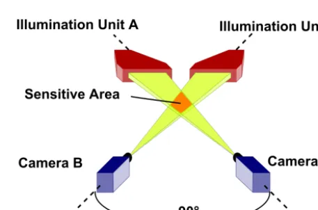
Figure 2. Measurement principle of the 2-DVD (modified from Kruger and Krajewski, 2002).
these lines to a complete picture delivers shape information for every single hydrometeor. A detailed description of an earlier version of the 2-DVD and an investigation on its po-tential in measuring rain parameters can be found in Kruger and Krajewski (2002). The smaller housing design of the compact 2-DVD makes it less sensitive to horizontal winds. Nevertheless, there is still the problem that horizontal wind fields can cause horizontal distortion of the spatial distribu-tion of hydrometeors inside the measuring area and the 2-DVD pictures themselves. The manufacturer supplies a soft-ware which corrects the apparent canting angle induced by horizontal velocity components for raindrops. This software was not used in the present study, because it does not apply for solid-phase precipitation. Nešpor et al. (2000) showed that horizontal wind components which exist in the direct vicinity of the 2-DVD housing can influence the measure-ment of drop-size distributions significantly, especially for smaller hydrometeors. For this reason the measurements pre-sented in the following were conducted under calm wind con-ditions with wind velocities below 5.0 m s−1. The cameras built in the 2-DVD which is used in the present study scan a line containing 632 pixels with a frequency of 55.272 kHz, which results in a higher spatial resolution.
2.2 The matching problem
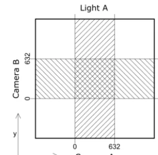
Every hydrometeor that falls through the 2-DVD within the shaded areas (see Fig. 3) is seen by at least one camera. But only hydrometeors that are seen by both cameras (cross shaded area) can be used for subsequent data analysis. The most critical step in processing 2-DVD raw data is finding exactly that pair of pictures that belongs to the same hydrom-eteor. This process is called matching. In contrast to rain, where a well-known symmetry and size–velocity relation can be assumed, the shapes of solid-phase and mixed-phase hy-drometeors are more complex. This makes it more difficult to find a pair of 2-DVD images that belong to the same hydrom-eteor. Without implementing an appropriate matching algo-rithm, the probability of errors in shape and velocity mea-surement through matching artifacts is very high. To find the right matching partner to a picture recorded in camera A, a time window has to be defined in which the matching part-ner has to appear in camera B. The narrower the time win-dow, the higher the probability of finding the right match is. Raindrops have a well-known relationship between their size and terminal fall velocity (Gunn and Kinzer, 1949; At-las et al., 1973), and the time window can be set very narrow. In case of solid-phase precipitation the fall velocity is lower than for liquid-phase hydrometeors. Complex surface struc-tures increase drag forces, and the vertical fall velocity for solid-phase hydrometeors depends not only on size but also on shape and degree of riming (Locatelli and Hobbs, 1974; Barthazy and Schefold, 2006).
A first attempt of solving the matching problem for snow measurements was done by Hanesch (1999). In this study the
Figure 3. A schematic view of the 2-DVD measuring area seen from above.
approach of Huang et al. (2010) was applied with few modi-fications. In principle, several ranges of parameters were de-fined in which the hydrometeors must match to be identified as a single one. Huang et al. (2010) set a fixed velocity range from 0.5 to 6.0 m s−1for the whole size range. In this work a dynamic upper-bound velocity is used for each hydrome-teor with the widthw. It is set to the velocityv(w), which a raindrop with widthwwould have (Atlas et al., 1973): v(w)=9.65−10.3·e−0.6·w. (1) This adjustment makes sure that also partially melted and mixed-phase hydrometeors can be matched. Figure 4 sum-marizes the size–velocity relationships for different types of hydrometeors in a size range from 0.5 to 8.0 mm as deter-mined by several investigators. It justifies the assumption of Eq. (1) as an upper limit.
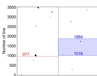
With the known scan frequency this time window can be translated into an interval of lines in camera B that has to contain the right matching partner (see the shaded region in Fig. 5). In the example from Fig. 5 three possible matching partners are found within the shaded region. Three so-called matching factors are now calculated for each pair of pictures:
– f1=1−max|SL(SLA−ASL,SLB|B)
withSLA/B: number of scanned lines in camera A and B
– ifF ≤1:f2=F, else:f2=2−F withF = min(Wmax,Hmax)
0.8·max(Wmax,Hmax) – f3=Wmin/Wmax.
Figure 4. Size–velocity relationships for different types of hydrom-eteors as reported in literature. The term size means diameter in case of rain; in case of snow it means height or maximum dimension.
Figure 5. This example shows two raw camera streams. For the spe-cific snowflake hitting camera A at the red line, all possible match-ing partners in camera B are within the shaded region.
It is worth mentioning that in this study the newly imple-mented matching algorithm is applied directly to the raw data streams coming from the cameras. The original matching al-gorithm supplied by the manufacturer (hereafter referred to as original matching algorithm) is explicitly not used for the data analysis in this work. Therefore the algorithm used in this study is not called rematching. But in the studies from Huang et al. (2010) and Grazioli et al. (2014) the term re-matching lets the reader assume that the original algorithm is used in some stage.
2.3 Size, velocity and shape parameters
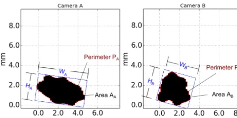
The result of the matching software is a pair of pictures from each hydrometeor falling through the sensitive area. The great advantage of the 2-DVD is that a very detailed set of parameters can be derived from two orthogonal views. For each picture, width (W), height (H), perimeter (P) and area (A) can be defined as in Fig. 6. A set of shape characterizing parameters can be assigned to each component of a 2-DVD image pair. This work deals with three dimensionless fac-tors which are commonly used in land use analysis (Jiao and Liu, 2012) and recently also in snow classification (Grazioli et al., 2014). Among the potential descriptors for hydrome-teors (Grazioli et al., 2014) we have chosen those which we found to be useful to characterize aerosol scavenging.
a. Elongation:E=max(W,H ) min(W,H )
The elongation describes the ratio between width W and heightH. The more elongated a hydrometeor is, the largerEis. Needles have a large elongation. Rain or graupel particles have lower elongations than other types of hydrometeors.
b. Roundness:R= 4A
π(max(W,H ))2
The roundness is a quantity that describes how well the hydrometeor fills out the area that is enclosed in the circumscribing circle. Needles and dendrites have a low roundness. Rain or graupel particles are expected to have a larger roundness than other types of hydrome-teors.
c. Shape factor:S=4π A
P2
The shape factor sets the surface area of a particle in re-lation to its perimeter. An ideally spherical particle has a shape factor of 1. The lower the shape factor, the more complex the surface of the particle is. Flakes or den-drites have a low shape factor. The shape factor of rain and graupel particles is expected to be larger than the one for other types of hydrometeors.
Another, size describing, set of parameters can be derived with the combination of both camera pictures:
d. The maximum dimension D (mm) is the maximum value of width and height seen in both cameras. e. The volume V (mm3) of a hydrometeor is calculated
the following way: every line scan cuts the hydrometeor into slices. The volume of each slice is defined by the area of an ellipse with the length of the shadowed line in each camera as a semi-axis and the height of the line. The sum of these volumes is the volume of the hydrom-eteor (Schönhuber, 1998).
Figure 6. The definition of width (W), height (H), perimeter (P) and area (A) for a hydrometeor as recorded with the 2-DVD
g. The vertical fall velocityv(D)(m s−1) is the exact plane distance at the (x,y) location of the hydrometeor in the sensitive area divided by the time interval from the first hit in camera A to the first hit in camera B.
An ensemble of hydrometeors that fell during a certain time interval is described with mean values of the mentioned microscopic parameters.
2.4 Experimental methods
Possible misalignment of the optical components due to transport, strong winds and the use of a new data analysis software motivate a recalibration of the device in addition to the calibration done by the manufacturer: steel spheres with diameters from 0.5 to 10 mm were dropped through the measuring area. For each size, between 30 and 70 calibration spheres were released from the same height (0.52 m) above the first camera plane; the values for height and width mea-sured in camera A and B were compared to the known nom-inal values for the spheres. For the determination of the size of an object the pixel widthphas to be known. It is defined as the actual width of a shaded line divided by the number of shaded pixelsnpixand depends on the exactxandyposition of the object and on a size-dependent correction factorfcorr supplied by the manufacturer. Because of the individual po-sitions in the sensitive area, every detected object has its own pixel widthp:
p=p(x, y)·fcorr. (2)
p(x, y)denotes the width of a single camera pixel seen from the location (x, y).fcorr is the individual correction factor supplied by the manufacturer. Dropping solid spheres from a known height through the sensitive area is also suitable for verification of shape and velocity measurements because of the following reasons:
– The real values of elongation (E), roundness (R) and shape factor (S) are easily determined asE=R=S= 1.
– The real values of elongation, roundness and shape fac-tor are independent of the orientation of the object to the recording camera, which makes the experiment eas-ily reproducible.
– For spherical objects the expected velocity after a cer-tain distance of free fall can be calculated solving the equation of motion
mdv
dt =mg− 1 2ρCDAv
2 (3)
for Reynolds numbers, Re, between 100 and 2000.m, v and Aare the mass (kg), velocity (m s−1) and sur-face area (m2) of the falling object respectively. g is the gravitational acceleration (m s−2) and ρ the air density (kg m−3). The drag coefficientCD depends on the Reynolds number and varies approximately linearly from 1.0 for Re=100 to 0.35 for Re=2000.
The originally implemented analysis software for solid-phase precipitation supplied by the manufacturer was evalu-ated in the following way: as an example a real snowfall event was analyzed with the original matching algorithm on the one hand and the established criteria after Hanesch (1999) (see Table 1) on the other hand. These are mainly geometric criteria which snowflakes must fulfill. In addition, particles with velocities larger than 6.0 m s−1(which is not reasonable for snow) were sorted out.
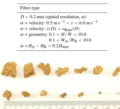
For the evaluation of the performance of the new match-ing algorithm, a reproducible experiment with fallmatch-ing objects that behave like solid- or mixed-phase precipitation particles was performed. Fourteen irregularly shaped Styrofoam par-ticles with different maximum dimensions from 2 to 15 mm (Fig. 7) were dropped through the sensitive area one after the other. This was repeated five times and the mean value of the measured fall velocity was calculated for each size. In a second step an ensemble consisting of 42 Styrofoam par-ticles within the same size range was released at the same time from the same height as in the first step. The second step was repeated several times; for data evaluation, a case was chosen where most of the particles contained in the en-semble fully hit the sensitive area. By comparing the mea-sured velocities in the second step to those from the first step mismatches can easily be identified. The Styrofoam particles were coated with a stabilizing spray color to avoid breaking of the particles when they hit the ground. A mean density of 270.0 kg m−3was measured for the particles.
Table 1. Filter criteria for the test of the original matching algorithm (adapted from Hanesch, 1999). D is the maximum dimension,v the vertical velocity andHA/BandWA/Bare the width and height measured in camera A and B.
Filter type
D >0.2 mm (spatial resolution, sr) sr+velocity: 0.5 m s−1< v <6.0 m s−1 sr+velocity:v(D) < vRain(D)
sr+geometry: 0.1< H /W <10.0 0.1< WA/WB<10.0 sr+HA−HB<0.2Hmax
Figure 7. Fourteen Styrofoam particles with maximum dimensions from 2 to 15 mm simulate solid hydrometeors to validate the match-ing algorithm
crystals or more of simply shaped pellets or graupel particles. Intervals with high mean elongation are expected to have low mean roundness and low mean shape factor and vice versa. Intervals with a low mean shape factor should also have a low mean roundness. Testing whether this behavior can be re-produced in 2-DVD measurements gives information on the self-consistency of the instrument when real snowfall events are recorded.
3 Results 3.1 Calibration
The calibration experiment for the height and width measure-ments with solid spheres shows that mean height and width are overestimated constantly (Fig. 8, left panel). As sum-marized in Table 2 the overestimation ranges from 0.35 to 0.38 mm. mandt denote the slope and intercept of the re-gression line, respectively.ris the correlation coefficient.
The right panel in Fig. 8 shows the results of the size mea-surements after implementing the following equation as a correction of the pixel width:
p=p(x, y)·fcorr−t /npix. (4)
p(x, y)denotes the width of a single camera pixel seen from the location(x, y).fcorris the correction factor supplied by
Figure 8. Comparison between nominal and measured height of calibration spheres before and after correcting the pixel width.
Table 2. Results of the calibration measurements with steel spheres. mandtdenote the slope and intercept of the regression line, respec-tively.ris the correlation coefficient.HA/BandWA/Bare the width and height measured in camera A and B.
m t r2
HA 1.04 0.35 0.998 HB 1.03 0.38 0.998 WA 1.04 0.35 0.998 WB 1.03 0.37 0.998
the manufacturer.t is the intercept as it can be found in Ta-ble 2 andnpixis the number of shaded pixels. There is good agreement between measured and nominal height for cam-era A.
3.2 Measurement ranges and uncertainties
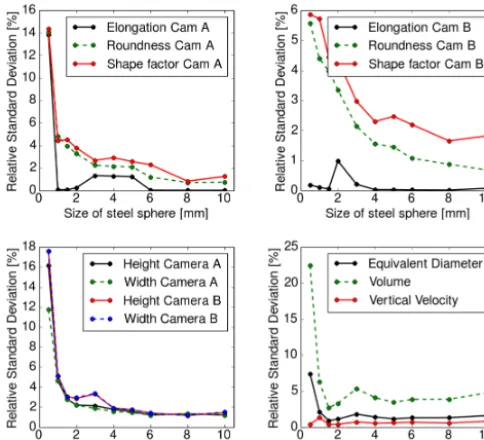
For the experiments with solid spheres the relative standard deviation for each parameter (Sect. 2.3 a to g) can be cal-culated (Fig. 9). It varies for the elongation, roundness and shape factor in camera A from 14 % for spheres with a diam-eter of 0.5 mm to 1.7 % for spheres with a diamdiam-eter of 10 mm. In camera B it varies from 6 to 2 %. The height and width can be measured with a relative standard deviation between 18 % for small particles and 1.8 % for larger ones in both cameras. The relative standard deviation for equivalent diameter and volume vary from 7 to 1.5 % and from 22 to 5 %, respec-tively. For the vertical velocity it stays below 1.5 % in the observed size range. An important parameter for the whole data analysis procedure is the spatial resolution or the width of a single pixel. Depending on thexandycoordinate of the hydrometeor in the measuring plane (see Fig. 3) for the in-strument used in this study, the single pixel width varies from 0.15 to 0.25 mm pixel−1.
3.3 Validation of 2-DVD measurements
Figure 9. The relative standard deviation for the different quantities measured with steel spheres.
a. The 2-DVD measures elongations very close toE=1 (Fig. 10a and b). At 0.5, 2, 3, 4 and 5 mm outliers can be identified.
b. The measured roundness values are very close toR=1. The spread of the single measurements gets higher for smaller spheres (Fig. 10c and d).
c. Figure 10e and f show the shape factors measured for the calibration spheres. They are between 0.6 and 0.7. Using a blurring edge filter from the software package OpenCV (2015) that spreads over 20 pixels before de-tecting the perimeter of the object, values between 0.90 and 0.95 are measured (Fig. 10g and h).
d. The slopem and intercept t for the linear regression line between nominal and measured maximum dimen-sion arem=1.04 andt= −0.01 (Fig. 8).
e. Equivalent diameters (Fig. 11a) and
f. volumes are reproduced very well in 2-DVD measure-ments (Fig. 11b).
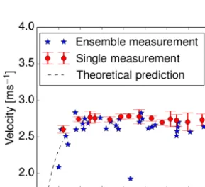
g. Measurements of the fall velocity show a very low spread around the theoretically predicted values (Fig. 11c).
Testing the new matching algorithm with an ensemble of Styrofoam particles shows the following result. An ensemble consisting of 42 Styrofoam particles was released at the same time. As one example, the results of an experiment where 30 particles fully hit the sensitive area is shown (Fig. 12).
Figure 10. Comparison between measured and expected values for the shape parameters. Elongation (a, b), roundness (c, d), shape fac-tor with (g, h) and without (e, f) treatment with a blurring edge filter.
The velocities measured in the ensemble (ensemble measure-ments) were compared to those measured when every parti-cle was dropped one after the other (single measurements). The ensemble measurements have a very low spread around the single measurements. The measured velocities are be-tween 2.0 and 2.9 m s−1. Out of 30 detected particles only for the size between 8 and 9 mm, one outlier was detected.
Figure 11. Comparison between measured and expected values for equivalent diameter (a), volume (b) and vertical velocity (c).
Figure 12. Comparison of velocity measurements of single Styro-foam objects (dropped one after the other) and of the whole ensem-ble (all particles dropped at the same time from the same height).
Table 3. Contribution of detected hydrometeors after applying the original matching algorithm.Dis the maximum dimension,vthe vertical velocity andHA/BandWA/Bare the width and height mea-sured in camera A and B.
Filter type Remaining %
number of flakes
Total (no filter) 439 072 100
D >0.2 mm (spatial resolution, sr) 178 949 40.8 sr+velocity: 0.5m s−1< v <6.0m s−1 142 299 32.4 sr+velocity:v(D) < vRain(D) 111 896 25.5 sr+geometry: 0.1< H /W <10.0
0.1< WA/WB<10.0 86 185 19.6 sr+HA−HB<0.2Hmax 38 677 8.8
same maximum dimension would have. Finally 9 % of hy-drometeors fulfill the criterion that the height measured in camera A is not more than 20 % different to the height mea-sured in camera B (Table 3).
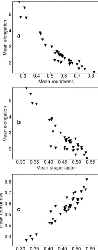
Figure 13a–c summarize the performance evaluation in case of real solid-phase precipitation. The measured mean shape parameters show the following correlations: higher elongation means lower roundness and shape factor. Lower elongation means higher roundness and shape factor. Inter-vals with lower roundness also have lower shape factors and vice versa.
4 Discussion 4.1 Calibration
The reason for the systematic deviation registered in the cal-ibration experiment can be a small misalignment of the opti-cal elements caused by transportation or small deformations of the housing through strong winds. Because of the con-stant overestimation of the measured quantity expressed in the interceptt of the regression line a correction procedure is implemented for the pixel width. After the correction the nominal and measured values agree very well (Fig. 8). The mentioned deviation in the size measurement leads to the rec-ommendation to all 2-DVD users to recalibrate their instru-ment periodically. The half-yearly calibration of the plane distance which is recommended by the manufacturer should be supplemented with a test of the size calibration.
4.2 Measurement ranges and uncertainties
Figure 13. Comparison between mean shape parameters measured for real snowflakes. Higher elongation means lower roundness (a) and lower shape factor (b), lower roundness means lower shape fac-tor (c) (and vice versa).
a maximum dimension of at least 0.5 mm for data evaluation. Size and shape characterization with a relative standard devi-ation of less than 5 % is only possible for particles larger than 1 mm. For particles between 0.5 and 1.0 mm the relative stan-dard deviation can grow up to 22 % for the volume, 17 % for size parameters and 14 % for shape descriptors. The relative standard deviation was calculated by dividing the absolute standard deviation by the mean value of the analyzed param-eter. For the size-related quantities, this can also be one rea-son for increasing relative standard deviation with decreasing size.
4.3 Validation of 2-DVD measurements
The measurement results with the solid spheres reveal how well shape, size and velocity information, gained with 2-DVD measurements, reproduce the reality.
a. The expected value of the elongationE=1 is repro-duced very well by the 2-DVD measurements (Fig. 10a and b). The outliers at 0.5, 2, 3, 4 and 5 mm are single measurements where partially shadowed edge pixels ar-tificially increase the width.
b. Especially for the larger spheres the expected roundness value ofR=1 is reproduced very well. With smaller diameters the influence of the pixel shaped edge gets larger. As a consequence the measured shape deviates more from a sphere and the values are spread more widely (Fig. 10c and d).
c. The expected value for the shape factor of a sphere is S=1. The measured values are between 0.6 and 0.7. The reason for this deviation is the pixel shaped perime-ter of the pictures. The perimeperime-ter of a convex pixel shaped object is always equal to the perimeter of the surrounding rectangle. For example a spherical object with a pixel shaped edge and a diameter of 6 mm has a theoretically calculated shape factor of 0.62. Using a blurring edge filter from the software package OpenCV (2015) that spreads over 20 pixels before detecting the perimeter of the object improves the shape factors to values between 0.90 and 0.95 (Fig. 10e to h). Especially for solid-precipitation particles with very fine features image processing with a blurring edge filter is not rec-ommended. The risk of losing important information is too high.
d. The measurement quality of the maximum dimension (Fig. 8),
e. equivalent diameters (Fig. 11a) and
f. volumes is excellent for particles larger than 0.5 mm (Fig. 11b).
g. The comparison between measured and theoretically calculated vertical fall velocity shows very good agree-ment (Fig. 11c).
In the experiment with Styrofoam particles, the mismatch probability was below 3 %. For particles with sizes below 3 mm the theoretical prediction for spherical particles with a density of 270.0 kg m−3is plotted in Fig. 12. The particles with sizes around 2 mm follow this prediction very well. The measured size and velocity depends strongly on the orienta-tion of the particle. For this reason a small spread around the single measurements has to be accepted.
algorithm produces a large number of mismatches. Less than 9 % of the registered events fulfill the criteria to be simultane-ously detected hydrometeors by both cameras (Table 3). For shape parameter measurements in case of real solid-phase precipitation, the 2-DVD shows the expected correlations (Fig. 13a–c).
5 Conclusion
This work was dedicated to the investigation of the con-sistency of 2-D video disdrometer measurements regarding size, shape and velocity parameters which are used for the characterization of solid hydrometeors. Results from exper-iments with solid spheres reproduced well-known nominal values for size, shape and velocity parameters convincingly. Taking the shape factor for shape characterization of hy-drometeors, it is important to consider the large influence of the pixel shaped perimeter. Further reproducible exper-iments with irregularly shaped objects suitable to simulate snowflakes are proposed. These experiments should espe-cially concern the reproducibility of bulk size, shape and ve-locity parameters in ensembles of identically shaped objects. The user of 2-D video disdrometer devices should keep in mind that size and shape characterization with a relative stan-dard deviation of less than 5 % is only possible for particles larger than 1 mm.
A second aim of the work was to highlight the need of a suitable matching algorithm for the measurement of mixed-and solid-phase precipitation. Because of the high number of matching artifacts, the originally distributed matching al-gorithm is not suitable for mixed- and solid-phase precipita-tion. In experiments with irregularly shaped Styrofoam parti-cles, the approach of Hanesch (1999) and Huang et al. (2010) was proved to be suitable for the measurement of solid- and mixed-phase precipitation. It is essential to implement a suit-able matching algorithm to avoid errors in shape and velocity measurements through matching artifacts.
Acknowledgements. We thank the staff of UFS Schneefernerhaus for assistance in the operation of the 2-DVD.
The study was supported by the German Ministry of Science and Education (BMBF) under contract 02NUK015B. Its contents are solely the responsibility of the authors.
Edited by: M. Kulie
References
Atlas, D., Shrivastava, R., and Sekhon, R.: Doppler radar character-istics of precipitation at vertical incidence, Rev. Geophys. Space Ge., 11, 1–35, 1973.
Barthazy, E. and Schefold, R.: Fall velocity of snowflakes of differ-ent riming degree and crystal types, Atmos. Res., 82, 391–398, 2006.
Barthazy, E., Goke, S., Schefold, R., and Högl, D.: An Optical Ar-ray Instrument for Shape and Fall Velocity Measurements of Hy-drometeors, J. Atmos. Ocean. Tech., 21, 1400–1416, 2004. Battaglia, A., Rustmeier, E., Tokay, A., Blahak, U., and Simmer,
C.: PARSIVEL Snow Observations: A Critical Assessment, J. Atmos. Ocean. Tech., 27, 333–344, 2010.
Brandes, E. A., Ikeda, K., Zhang, G., Schönhuber, M., and Ras-mussen, R. M.: A Statistical and Physical Description of Hy-drometeor Distributions in Colorado Snowstorms Using a Video Disdrometer, J. Appl. Meteorol. Clim., 46, 634–650, 2007. Cao, Q., Zhang, G. F., Brandes, E., Schuur, T., Ryzhkov, A., and
Ikeda, K.: Analysis of video disdrometer and polarimetric radar data to characterize rain microphysics in Oklahoma, J. Appl. Me-teorol. Clim., 47, 2238–2255, 2008.
Feind, R. E.: Comparison of three classification methodologies for 2-D probe hydrometeor images obtained from the armored T-28 aircraft, Tech. rep., Institute of Atmospheric Sciences, South Dakota School of Mines and Technology, Rapid City, SD, USA, tech. Rep. SDSMT/IAS/R08-01, 2008.
Frank, G., Härtl, T., and Tschiersch, J.: The pluviospectrometer: classification of falling hydrometeors via digital image process-ing, Atmos. Res., 34, 367–378, 1994.
Grazioli, J., Tuia, D., Monhart, S., Schneebeli, M., Raupach, T., and Berne, A.: Hydrometeor classification from two-dimensional video disdrometer data, Atmos. Meas. Tech., 7, 2869–2882, doi:10.5194/amt-7-2869-2014, 2014.
Gunn, R. and Kinzer, G. D.: The terminal velocity of fall for water droplets in stagnant air, J. Meteorol., 6, 243–248, 1949. Hanesch, M.: Fall Velocity and Shape of Snowflakes, PhD thesis,
Swiss Federal Institute of Technology, Zürich, Switzerland, (Su-pervisor: A. Waldvogel), 1999.
Hiroshi, I.: Radar backscattering computations for fractalshaped snowflakes, J. Meteorol. Soc. Jpn., 86, 459–469, 2008.
Hong, G.: Radar backscattering properties of nonspherical ice crystals at 94 GHz, J. Geophys. Res., 112, D22203, doi:10.1029/2007JD008839, 2007.
Huang, G. J., Bringi, V. N., Cifelli, R., Hudak, D., and Petersen, W. A.: A methodology to derive radar reflectivity–liquid equiv-alent snow rate relations using C-band radar and a 2-D Video Disdrometer, J. Atmos. Ocean. Tech., 27, 637–651, 2010. Jiao, L. and Liu, Y.: Analyzing the shape characteristics of land use
classes in remote sensing imagery, ISPRS Annals of Photogram-metry, Remote Sens. Spatial Inf. Sci., I-7, 135–140, 2012. Kruger, A. and Krajewski, W. F.: Two-Dimensional Video
Disdrom-eter : A Description, J. Atmos. Ocean. Tech., 19, 602–617, 2002. Kyrö, E.-M., Grönholm, T., Vuollekoski, H., Virkkula, A., Kulmala, M., and Laakso, L.: Snow scavenging of ultrafine particles: field measurements and parameterization, Boreal Environ. Res., 6095, 527–538, 2009.
Locatelli, J. D. and Hobbs, P. V.: Fall speeds and masses of solid precipitation particles, J. Geophys. Res., 79, 2185–2197, 1974. Löffler-Mang, M. and Joss, J.: An optical disdrometer for measuring
size and velocity of hydrometeors, J. Atmos. Ocean. Tech., 17, 130–139, 2000.
OpenCV: OpenCV version 2.4.11.0 – documentation, available at: http://docs.opencv.org/index.html (last access: 9 June 2015), 2015.
Paramonov, M., Grönholm, T., and Virkkula, A.: Below-cloud scav-enging of aerosol particles by snow at an urban site in Finland, Boreal Environ. Res., 16, 304–320, 2011.
Schaefer, V. J.: The preparation of snow crystal replicas-VI, Weath-erwise, 9, 132–135, 1956.
Schönhuber, M.: About Interaction of Precipitation and Electro-magnetic Waves, PhD thesis, Technical University Graz, Austria (Supervisor: W. L. Randeu), 1998.
Schönhuber, M., Lammer, G., and Randeu, W. L.: The 2-D video disdrometer, in: Precipitation: Advances in Measurement, Es-timation and Prediction, edited by: Michaelides, S., Springer, Berlin, Germany, 2008.
Schuur, T. J., Ryzhkov, A. V., Zrnic, D. S., and Schonhuber, M.: Drop size distributions measured by a 2-D video disdrometer: Comparison with dual-polarization radar data, J. Appl. Meteo-rol., 40, 1019–1034, 2001.
Sportisse, B.: A review of parameterizations for modelling dry de-position and scavenging of radionuclides, Atmos. Environ., 41, 2683–2698, 2007.
Thurai, M. and Bringi, V. N.: Drop axis ratios from a 2-D video disdrometer, J. Atmos. Ocean. Tech., 22, 966–978, 2005. Thurai, M., Szakall, M., Bringi, V. N., Beard, K. V., Mitra, S., and
Borrmann, S.: Drop shapes and axis ratio distributions: compar-ison between 2-D video disdrometer and wind-tunnel measure-ments, J. Atmos. Ocean. Tech., 26, 1427–1432, 2009.
Thurai, M., Williams, C. R., and Bringi, V. N.: Examining the corre-lations between drop size distribution parameters using data from two side-by-side 2-D-video disdrometers, Atmos. Res., 144, 95– 110, 2014.
Tokay, A., Kruger, A., and Krajewski, W. F.: Comparison of Drop Size Distribution Measurements by Impact and Optical Disdrom-eters, J. Appl. Meteorol., 40, 2083–2097, 2001.
Woods, C. P., Stoelinga, M. T., and Locatelli, J. D.: The IMPROVE-1 storm of IMPROVE-1–2 February 200IMPROVE-1. Part III: Sensitivity of a mesoscale model simulation to the representation of snow particle types and testing of a bulk microphysical scheme with snow habit predic-tion, J. Atmos. Sci., 64, 3927–3948, 2007.
Xue, M., Droegemeier, K. K., and Wong, V.: The Advanced Re-gional Prediction System (ARPS); A multi-scale nonhydrostatic atmospheric simulation and prediction model. Part I: model dy-namics and verification, Meteorol. Atmos. Phys., 75, 161–193, 2000.
Zhang, G., Xue, M., Cao, Q., and Dawson, D.: Diagnosing the in-tercept parameter for exponential raindrop size distribution based on video disdrometer observations: model development, J. Appl. Meteorol. Clim., 47, 2983–2992, 2008.
Zhang, G., Luchs, S., Ryzhkov, A., and Xue, M.: Winter Precip-itation Microphysics Characterized by Polarimetric Radar and Video Disdrometer Observations in Central Oklahoma, J. Appl. Meteorol. Clim., 50, 1558–1570, 2011.