www.atmos-meas-tech.net/5/1551/2012/ doi:10.5194/amt-5-1551-2012
© Author(s) 2012. CC Attribution 3.0 License.
Measurement
Techniques
Seven years of global retrieval of cloud properties using space-borne
data of GOME
L. Lelli1, A. A. Kokhanovsky1, V. V. Rozanov1, M. Vountas1, A. M. Sayer*,2,3, and J. P. Burrows1
1Institute of Environmental Physics and Remote Sensing, University of Bremen, Otto-Hahn-Allee 1, 28334 Bremen, Germany 2Atmospheric, Oceanic & Planetary Physics, University of Oxford, Oxford, UK
3Remote Sensing Group, STFC Rutherford Appleton Laboratory, Chilton, UK
*now at: Goddard Earth Sciences Technology And Research (GESTAR), NASA Goddard Space Flight Center,
Greenbelt, MD 20771, USA
Correspondence to: L. Lelli ([email protected])
Received: 8 July 2011 – Published in Atmos. Meas. Tech. Discuss.: 4 August 2011 Revised: 24 May 2012 – Accepted: 8 June 2012 – Published: 10 July 2012
Abstract. We present a global and regional multi-annual (June 1996–May 2003) analysis of cloud properties (spher-ical cloud albedo – CA, cloud opt(spher-ical thickness – COT and cloud top height – CTH) of optically thick (COT>5) clouds, derived using measurements from the GOME instrument on board the ESA ERS-2 space platform. We focus on cloud top height, which is obtained from top-of-atmosphere backscat-tered solar light measurements in the O2A-band using the
Semi-Analytical CloUd Retrieval Algorithm SACURA. The physical framework relies on the asymptotic equations of radiative transfer. The dataset has been validated against independent ground- and satellite-based retrievals and is aimed to support trace-gases retrievals as well as to cre-ate a robust long-term climatology together with SCIA-MACHY and GOME-2 ensuing retrievals. We observed the El Ni˜no-Southern Oscillation anomaly in the 1997–1998 record through CTH values over the Pacific Ocean. The global average CTH as derived from GOME is 5.6±3.2 km, for a corresponding average COT of 19.1±13.9.
1 Introduction
Clouds play an important role in the Earth climate system (Stephens, 2005; Heintzenberg and Charlson, 2009). The amount of radiation reflected by the Earth-atmosphere sys-tem into outer space depends not only on the cloud cover and the total amount of condensed water in the atmosphere but also on the size of droplets and their thermodynamic
state. The information about microphysical properties, cloud top height and spatial distributions of terrestrial clouds on a global scale can be obtained optimally with satellite re-mote sensing systems. The amount of reflected solar light de-pends both on geometrical and microphysical characteristics of clouds. In particular, it is often assumed that clouds can be represented by homogeneous and (in horizontal direction) infinitely extended plane-parallel slabs. The range of appli-cability of such an assumption for real clouds is limited be-cause 3-D effects are not taken into account and multi-layer cloud systems can occur. However some properties can still be derived and valuable information can be retrieved.
Table 1. Relevant cloud datasets from the respective passive satellite imagers, retrieval approaches and products. Acronyms: CTP (Cloud Top Pressure), CF (Cloud Fraction), CER (Cloud Effective Radius), COT (Cloud Optical Thickness), CA (Cloud Albedo), CWP (Cloud Water Path), CPI (Cloud Phase Index), LWP (Liquid Water Path).
Instrument Spectral channels (µm) and method Record length Cloud product Reference
ISCCP 0.5–11, Threshold 25 yr CF, CTP, COT, CER, CWP Rossow and Schiffer (1999)
HIRS 13.3–14.2, CO2-slicing 23 yr CF, CTP Wylie and Menzel (1999)
AVHRR 0.63, 0.83, 3.7, 10.8, 12, Threshold 20 yr CF Jacobowitz et al. (2003)
ATSR 0.55, 0.67, 0.87, 1.6 14 yr CF, CTP, COT Sayer et al. (2011)
3.7, 11, 12, IR-brightness temperature CER, CWP
MODIS 11, 13.3–15, CO2-slicing 12 yr CF, CTP, CER, COT, LWP Menzel et al. (2008) MISR 0.44, 0.55, 0.67, 0.86, stereo-matching 12 yr CF, CTH, CA Moroney et al. (2002) AIRS 10.9–14.19, CO2-χ2weighted 6 yr CF, CTH, CWP Stubenrauch et al. (2010)
OMI 0.475, O2-O2 6 yr CF, CTP Sneep et al. (2008); Vasilkov et al. (2008)
0.392–0.398 Rotational Raman Scattering
GOME/GOME-2 0.76, O2A-band, Neural Network 7 yr CF, CTH, COT, CA Loyola et al. (2010) (ROCINN) SCIAMACHY 0.76, 1.55, 1.67, O2A-band, asymptotic 10 yr CF, CTH, COT, CA, CER, CPI, LWP Kokhanovsky et al. (2007d) (SACURA)
GOME 0.76 O2A-band, asymptotic 7 yr CF, CTH, COT, CA This paper (SNGome)
GOME/SCIAMACHY/GOME-2 0.76, O2A-band 16 yr CF, CTH Wang et al. (2008) (FRESCO)
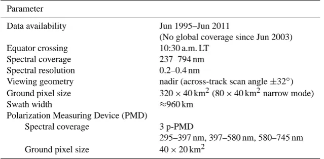
Table 2. GOME instrument technical specifications.
Parameter
Data availability Jun 1995–Jun 2011
(No global coverage since Jun 2003)
Equator crossing 10:30 a.m. LT
Spectral coverage 237–794 nm
Spectral resolution 0.2–0.4 nm
Viewing geometry nadir (across-track scan angle±32◦) Ground pixel size 320×40 km2(80×40 km2narrow mode)
Swath width ≈960 km
Polarization Measuring Device (PMD)
Spectral coverage 3 p-PMD
295–397 nm, 397–580 nm, 580–745 nm Ground pixel size 40×20 km2
Parameters and Evaluation (GRAPE, Poulsen et al., 2011; Sayer et al., 2011), the Multiangle Imaging SpectroRadiome-ter (MISR, Diner et al., 1989; Moroney et al., 2002), the Moderate Resolution Imaging Spectroradiometer (MODIS, Platnick et al., 2003; Menzel et al., 2008), the Atmospheric Infrared Sounder (AIRS, Stubenrauch et al., 2010) the Ozone Monitoring Instrument (OMI, Sneep et al., 2008; Vasilkov et al., 2008; Joiner et al., 2012), and the Scanning Imag-ing Absorption Spectrometer for Atmospheric Chartogra-phy (SCIAMACHY, Bovensmann et al., 1999; Kokhanovsky et al., 2007d).
Existing cloud datasets derived by measurements in the O2A-band are the Fast Retrieval Scheme for Clouds from
the Oxygen A-band (FRESCO, Wang et al., 2008, see http: //www.temis.nl/fresco/) and the Retrieval of Cloud Infor-mation using Neural Network (ROCINN, Loyola et al., 2010). New perspectives for cloud properties retrieval are offered by active sensors such as the Cloud Profiling Radar (CPR, Stephens et al., 2008) onboard CloudSat and the Cloud-Aerosol Lidar with Orthogonal Polarization (CALIOP, Winker et al., 2007) onboard CALIPSO platform.
In these systems, the high vertical resolution is counterbal-anced by the limited spatial coverage.
Though the main scientific objective of GOME (Global Ozone Monitoring Experiment, Burrows et al., 1999) is the retrieval of trace gases (Coldewey-Egbers et al., 2005; Meijer et al., 2006; Van Roozendael et al., 2012), its measurements are also relevant for the study of cloud parameters. GOME is a space-borne spectrometer that has been flying on the Euro-pean Remote Sensing Satellite 2 (ERS-2, whose payload has been switched-off since July 2011) since April 1995. GOME measured reflected solar radiation in the wavelength range between 240 and 790 nm at a spectral resolution of 0.2 to 0.4 nm (see Table 2).
multiple scattering, as photons travel inside. The properties to be known are cloud albedo, optical thickness and top height.
The aim of this paper is to describe the retrieval of such properties with SNGome (SACURA – Semi-Analytical CloUd Retrieval Algorithm – Next Generation for GOME) and assess the quality of the dataset through validation and comparison with other algorithms, based on different phys-ical approaches. The structure of the paper is as follows. In Sect. 2 the algorithm is described. The solution of the for-ward and inverse problem is sketched as well as the exten-sion to global processing. Section 3 is devoted to validation, both synthetic error analysis and against radar measurements and other retrieval techniques. In Sect. 4 we show results and global cloud patterns. In the final section we draw some conclusions.
2 SNGome algorithm description
It has been extensively proven that cloud top height can be retrieved from measurements in the oxygen A-band (758– 778 nm) (Yamamoto and Wark, 1961; Saiedy et al., 1967; Fischer and Grassl, 1991; Kuze and Chance, 1994; Koele-meijer et al., 2001; Kuji and Nakajima, 2002; Rozanov and Kokhanovsky, 2004). When a cloud is idealized as a perfect reflector, every photon striking on the cloud top will be scat-tered back and will not be absorbed by O2molecules within
or below the cloud. So the depth of the absorption line de-creases as the cloud altitude inde-creases because most of the oxygen is located under the clouds.
In reality, two further aspects must be considered. First, the assumption of a cloud as a Lambertian diffuser with zero transmittance and fixed plane albedo leads to the un-derestimation of height, because smaller top-of-atmosphere (TOA) reflectances in the oxygen absorption band are mis-interpreted as lower cloud layers (firstly remarked by Saiedy et al., 1967). Gaseous absorption takes place throughout a cloud layer and does not stop at the cloud top. This effect has been proven in the context of the Optical Centroid Pressure (OCP) for OMI retrievals (Vasilkov et al., 2008; Sneep et al., 2008; Joiner et al., 2012). Second, it has been shown that the sole retrieval of top height will be biased low if no attempt is made to account for multiple scattering and its value will be closer to the altitude of the middle of the cloud (Ferlay et al., 2010). The SNGome algorithm is based on Semi-Analytical CloUd Retrieval Algorithm (SACURA, Kokhanovsky et al., 2003; Rozanov and Kokhanovsky, 2004). SACURA was originally developed at IUP Bremen for the application to SCIAMACHY measurements (Gottwald and Bovensmann, 2010; Burrows et al., 2011; Kokhanovsky et al., 2011). It consists of two parts: a forward semi-analytical parameter-ization of the cloud TOA reflection function and a numeri-cal minimization for the retrieval. An extensive description can be found in Kokhanovsky et al. (2003); Rozanov and
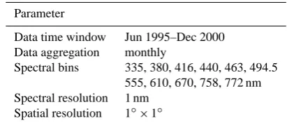
Table 3. TEMIS minimum Lambert-equivalent reflectivity database specifications.
Parameter
Data time window Jun 1995–Dec 2000 Data aggregation monthly
Spectral bins 335, 380, 416, 440, 463, 494.5 555, 610, 670, 758, 772 nm Spectral resolution 1 nm
Spatial resolution 1◦×1◦
Kokhanovsky (2004); Kokhanovsky and Rozanov (2004); Kokhanovsky and Nauss (2006).
2.1 The forward problem
The spectral top-of-atmosphere (TOA) reflectance is defined as
Rmes =
π I µ0E0
(1) where E0 is the spectral solar irradiance and µ0 the
co-sine of solar zenith angle. The geo-referenced calibrated and degradation-corrected spectral radiancesIare extracted from L0 GOME data with the aid of the GOME Data Processor 4 (Slijkhuis and Loyola, 2009). Due to the coarse GOME spa-tial resolution (i.e. 320×40 km2), two corrections are in-troduced to address the issue of broken cloudiness. It has been shown (Kokhanovsky et al., 2007a) that, as long as the cloud top height retrieval incorporates spectral ratios, the horizontal photon transport is of minor importance. Hence, if the cloud fraction value is known from an independent source, then it is reasonable to scale partially cloudy scenes to fully cloudy cases with the Independent Pixel Approxima-tion (IPA) (Marshak et al., 1995) and to calculate the cloud TOA reflectanceRclfrom
Rmes =cfRcl+(1−cf) Rs. (2)
The value of cloud fraction cf, defined as the fraction of
the GOME pixel occupied by a cloud, is delivered by DLR (Deutsches Zentrum f¨ur Luft- und Raumfahrt) in bundle with the GOME radiances and is based on the analysis of Po-larization Measuring Device (PMD) records (Loyola and Ruppert, 1998; Loyola, 2004). The clear sky reflectanceRs
is substituted by a Minimum Lambert-Equivalent Reflec-tivity (MLER) value taken from the global database Tro-pospheric Emission Monitoring Internet Service (TEMIS, Koelemeijer et al., 2003, see Table 3). This climatological value has been derived from 5.5 yr of GOME observations. The TEMIS sub-pixels are co-located (see Eqs. 1 and 2 in Kokhanovsky et al., 2007c) and averaged.
the surface is Lambertian with albedoA, is taken into ac-count with (see Eq. 54 in Kokhanovsky et al., 2003)
RTOA =R∞−t K0(µ) K0(µ0)+
A t2K0(µ) K0(µ0)
1−A (1−t ) , (3)
wheret is the cloud transmissivity,K0(µ) andK0(µ0)are
the escape functions,µandµ0 the cosines of viewing and
solar zenith angles andR∞the reflection function of an infi-nite layer, respectively. Arguments inR∞andRmesare
omit-ted for simplicity. The escape function can be approximaomit-ted as
K0(µ)=
3
7(1+2µ) (4)
with an accuracy of 2 % atµ>0.2 (Kokhanovsky, 2006). The value oftis related to the cloud optical thickness (COT)
τ via
t = 1
α+0.75τ (1−g). (5)
The asymmetry parameterg depends on the chosen phase function. We will assume thatg= 0.859 (i.e. water clouds, Kokhanovsky, 2006). The parameter α is almost indepen-dent of microphysics of clouds and is set equal to 1.07 (Kokhanovsky, 2006). The optical thicknessτ is then cal-culated from the continuum outside the absorption, at wave-length 758 nm, where almost no sensitivity to cloud top height is expected. Then it follows from Eqs. (3) and (5):
τ = 1−A−D (β−A) (α−1) 0.75D (1−A)(1−g) , D =
R∞−RTOA
K0(µ) K0(µ0)
, (6) whereβ=αα−1. This technique, used also in King (1987), ap-plies to clouds withτ >5. For the validation of cloud optical thickness, a set of MODIS Terra measurements was ingested and compared with two other algorithms (ATSK3/JAXA and MOD06/NASA, both based on look-up-tables approach. De-tails are given in Nauss et al., 2005). SACURA retrievals exhibit a slightly higher mean than MOD06 and ATSK3 (18.5 versus 15.9 and 16.9 respectively) and deviate±18 % on average from MOD06, with a stability indexr2of 0.99. Since the intercomparison has been performed on the same measurement set, the arose discrepancies among the algo-rithms rule out co-registration and scenario issues and can be tracked down to the different theoretical and algorithmic approaches.
The values of geometrical cloud heighthand thicknessl
are derived from measurements around the oxygen absorp-tion centered at 761 nm (whose depth as seen in reflected light depends also onτ), with the nominal GOME spectral resolution and sampling (67 spectral points were used). In this case, the modeled reflectanceRTOAis modified
account-ing for both gaseous absorption and multiple light scatteraccount-ing inside and below the cloud and has the following form
RTOA =R0+T1RbT2, (7)
where R0 gives the reflection function of the part of
at-mosphere above the cloud in the single scattering approx-imation. The Rayleigh and aerosol scattering and absorp-tion coefficients are considered. The aerosol properties are taken from MODTRAN 2/3-LOWTRAN 7 (Kneizys et al., 1996) and correspond to a tropospheric model with ground visibility 23 km and boundary layer humidity 70 %, while the stratospheric aerosol is the so-called background aerosol (Kneizys et al., 1996). Rb is the reflection function of the
cloud-underlying atmosphere system together with surface contribution, while the multipliersT1,2are the transmission
coefficients from the Sun to a cloud and from the cloud to a satellite, respectively. Accounting inT1,2only for gaseous
absorption (without aerosol and molecular extinction) dimin-ishes the total extinction along the light path and results in the increase of the second term of the right hand side of the above equation. This procedure enables the account of mul-tiple scattering above the cloud (Kokhanovsky and Rozanov, 2004). Moreover, the contribution of the atmospheric layer below the cloud is not neglected. Kokhanovsky and Rozanov (2004) illustrate how the aerosol-gaseous medium under the cloud and underlying surface can be approximated by an ef-fective Lambertian surface with albedoA.
The oxygen absorption within the cloud layer is taken into account in the term Rb. The main parameter is the
atmo-spheric single scattering albedo (SSA)ω0, which changes in
the presence of the cloud and depends on height inside the gaseous absorption band (Kokhanovsky and Rozanov, 2004). It can be written as
ω0=1−
σO2 abs
σext
, (8)
whereσO2
abs andσextare the oxygen absorption and the total
extinction coefficients, respectively. Aerosol and cloud ab-sorption in the visible are neglected. The value of the SSA for the effective homogeneous cloud layer is then calculated iteratively (the formulae are in Appendix A in Kokhanovsky and Rozanov, 2004). The accuracy of this approach is given in Yanovitskij (1997).
2.2 The inverse problem
The retrieval block of SNGome relies on the minimisation of the difference between the modelled and the observed TOA reflectances in the wavelength range 758–772 nm. It is as-sumed that the reflection functionR can be expanded in the Taylor series around the a-priori value of the cloud top height
h0as
R(h)=R (h0)+
∞ X
i=1
ai (h−h0)i and ai =
R(i)(h0)
i! (9) withR(i)(h0)being thei-th derivative ofR corresponding
to cloud top heighth0. It was found that the functionR(h)
change (Rozanov and Kokhanovsky, 2004). Therefore, ne-glecting nonlinear terms in Eq. (9), it follows
R(h)=R (h0)+R0(h0) (h−h0) and R0(h0)= dR dh h=h
0
. (10) Having set the value ofh0equal to 1.0 km, a value typical for
low level clouds, the actual cloud top heighthis calculated minimizing the cost function
F =
Rcl−R(h0)−R0(h0) (h−h0) 2
, (11) where Rclis the TOA reflectance calculated with Eq. (2).
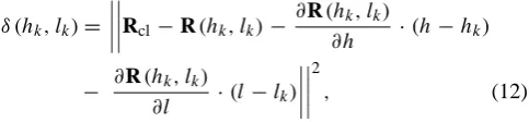
The retrieval of the pair (h,l) is accomplished writing a vectorial form of the above equation and performing a two-parameter minimization (Rozanov and Kokhanovsky, 2004). Tests have shown that the retrieval is almost insensitive to different start values of h0 and l0. This is due to the fact
that the solution for the two-parameter inverse problem is performed iteratively. In particular, the following values are set:h0= 1 km,l0= 100 m. The value of minimum difference
δ(hk, lk)between the forward calculated spectrum R and the
measured spectrum Rcl is iteratively looked for along the
whole absorption band with the following equation
δ (hk, lk)=
Rcl−R(hk, lk)−
∂R(hk, lk)
∂h ·(h−hk)
− ∂R(hk, lk)
∂l ·(l−lk)
2
, (12)
where the indexk= 0 ...Nis the needed iteration number. The retrieval of the cloud geometrical thicknesslenables the calculation of cloud bottom height (CBH). It reflects the transmission of light through a single-layered cloud and must be allowed to vary. The error analysis for CBH has been reported in Rozanov and Kokhanovsky (2004) and Lelli et al. (2011), where a black and a moderately bright surface (albedo 0.2) have been considered. What we see is that the values are accurate and stable for CTH and CBH values in range [1–16] km andτ values in range [5–50].
The correlated k-distribution accounts for the high-frequency oscillations of the oxygen molecular absorption coefficients. They are reproduced adopting the method of the “exponential sum fitting coefficients”: five precalculated profiles of molecular oxygen cross-section (T-,P- and λ -dependent) are employed, multiplied by tabulated constants, and summed up to give the convolved wavelength-dependent monochromatic TOA reflection function (Buchwitz et al., 2000). In this work, the wavelength step of 0.05 nm is used. This method enables fast calculations with an accu-racy within 2 % as compared with line-by-line calculations (Buchwitz et al., 2000). The temperature and pressure de-pendence of molecular absorption coefficients for a given lo-cation of measurements is accounted for using the standard atmosphere model (Br¨uhl and Crutzen, 1993).
Finally, the cloud spherical albedo r is calculated with the aid of Eq. (5), taking into account thatt= 1−r, if one
Table 4. SNGome quality flags.
Value Description
0 No retrieval
1 Only cloud bottom height convergence 2 Only cloud top height convergence 3 Geometrical thickness limit 4 No convergence
5 Cloud top and bottom height convergence
neglects absorption processes. The error forrhas been esti-mated smaller than 10 % atτ>6 and below 3 % atτ>10. The technique has been validated by comparing retrieved val-ues ofr with airborne measurements, showing remarkable agreement (Kokhanovsky et al., 2007b).
For global processing we employ the digital elevation model STRM30 (Earth Resources Observation and Science (EROS, USGS) Center, 2000). The fundamental sample spacing of 3 arc-second in latitude and longitude (≈90 m at equator) has been down-sampled to 0.5 arc-minute in both coordinates (≈1 km at equator).
The algorithm flags each retrieval in ascending order (see Table 4), depending on the quality of the simultaneous fits of cloud top and bottom height, given the value of cloud optical thickness calculated in the continuum outside the band.
In summary, the strengths of the algorithm are the semi-analytical forward parametrization of the TOA reflectances in the wavelength range of the oxygen A-band (but suitable to the broader range 0.4–2.4 µm) for clouds withτ >5 and solar zenith angles675◦, the inclusion of molecular, aerosol scattering in clear sky condition and multiple scattering in-side the cloud. In this way we avoid the common look-up-table approach.
3 Validation
3.1 Synthetic error analysis: single-layered cloud
The theoretical error investigation has been carried out gen-erating forward spectra with the radiative transfer software package SCIATRAN (v. 3.1, Rozanov et al., 2012) in the Scalar Discrete Ordinate Method (S-DOM) mode. This is be-cause polarization effect play a very little role in the O2
CTH absolute error, km
1 0.5 0
5 10 15 20 25 30 35 40 45 50 Cloud Optical Thickness
2 4 6 8 10 12 14 16
Cloud Top Height, km -0.4
-0.2 0 0.2 0.4
Fig. 1. Absolute error (in km) in the cloud top height retrieval with SNGome as function of cloud top height and optical thickness. Input parameters: solar zenith angle 60◦, nadir view, cloud geometrical thickness 1 km. The contour lines indicate the specified error levels (in km).
angle equal to 0◦. The absolute error of the retrieved top alti-tude, defined as
1=CTHretrieved−CTHforward,
is shown in Fig. 1. The error is in the expected value range (±0.5 km), in line with previous findings (Rozanov and Kokhanovsky, 2004), where the authors already pointed out the decreased sensitivity to oxygen absorption for high and thin clouds. However such clouds cannot be detected anyway by GOME, as reported in Rozanov et al. (2006).
Moreover, GOME is a UV-VIS instrument, lacking spec-tral coverage in the short-wave IR. This limitation implies the lack of information on the cloud phase function for the retrievals beforehand because only very weak absorption by condensed water takes place in UV-VIS; hence no cloud par-ticle size can be inferred. For this reason errors are intro-duced because the phase function can be only guessed and solar illumination geometry varies appreciably. Yet, in order to test the algorithm under realistic operational conditions, the choice has been to maintain a slight difference between the asymmetry parametersgin Eq. (5) used in the forward (g= 0.846) and inverse (g= 0.859) problem. This effect is de-picted in the cloud optical thickness retrieval, whose relative error is shown in Fig. 2. Given the geometry in Fig. 2, a so-lar zenith angle of 38◦corresponds to a scattering angle of 142◦. Referring to Kokhanovsky (2006, Fig. 37, p. 152), we are in the region of rainbow. An analytical error propagation study for a single spectral channel has been presented earlier by King (1987) and Kokhanovsky et al. (2003). For values of solar zenith angles→90◦,τ will be overestimated as a con-sequence of the increased light-path through the atmosphere, which weakens the assumption of the plane parallel geom-etry of our approach. In Fig. 3 the impact of bow regions is less evident. This error mitigation is due to the fact that only reflectances normalized to the average value of these functions outside the band (atλ= 758 nm) are ingested in the algorithm and that the retrieval itself is performed along the oxygen absorption band using 67 spectral points.
COT relative error, %
10 0 -10
0 10 20 30 40 50 60 70 80 Solar Zenith Angle, degree 0
0.1 0.2 0.3 0.4
Su
rf
a
ce
Al
b
e
d
o
-40 -20 0 20 40
Fig. 2. Relative error (%) in cloud optical thickness retrieval as function of surface albedo and solar zenith angle. Input parameters: COT 20, CTH 5 km, cloud geometrical thickness 1 km.
0 10 20 30 40 50 60 70 Solar Zenith Angle, degree 2
4 6 8 10 12 14 16
Cloud Top Height, km
-0.1 0 0.1 0.2 0.3 0.4 0.5 0.6 0.7 0.8 0.9
Fig. 3. As Fig. 1, but as a function of solar zenith angle in nadir view. Input parameters: COT 10, geometrical thickness 1 km.
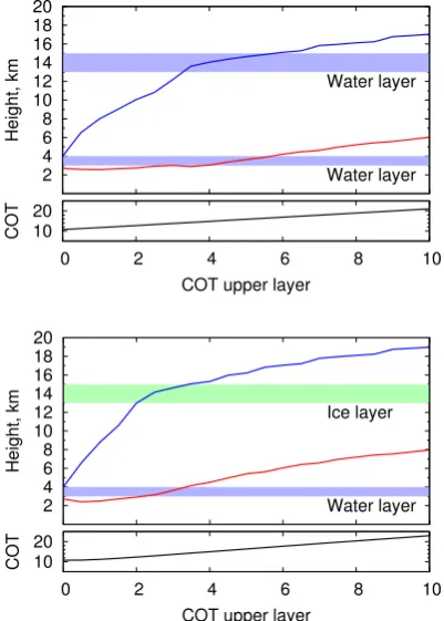
3.2 Synthetic error analysis: double-layered cloud
Addressing the issue of multi-layer clouds, which are likely to be sensed by GOME due to its spatial resolution, we have run synthetic tests for a two-layer system with a lower wa-ter cloud of COT = 10, CBH = 3 km, CTH = 4 km and the re-sults are shown in Fig. 4. In the first case, the upper wa-ter layer was fixed at heights 13–15 km; in the second case, an ice cloud was simulated with a fractal crystal model (Kokhanovsky, 2006) of 50 µm side length and placed at 13–15 km as well. This height value has been chosen from the CALIPSO dataset (Sassen et al., 2008). The solar zenith angle was set equal to 30◦, consistent with tropical lati-tudes. With increasing optical thickness of the upper layer, the curves show the cloud bottom (red curve) and top (blue curve) height retrieved values of the lower layer. The lower panel shows the total COT retrieved for both layers.
Inspecting the retrieval flags, we notice that the operational limit of geometrical thickness (11 km) is met at COTwater= 4
and COTice= 2 of the upper layer. Beyond that value, CTH
10 20
0 2 4 6 8 10
COT
COT upper layer 2
4 6 8 10 12 14 16 18 20
Height, km
Water layer Water layer
10 20
0 2 4 6 8 10
COT
COT upper layer 2
4 6 8 10 12 14 16 18 20
Height, km
Water layer Ice layer
Fig. 4. Retrieval of CTH (blue curves), CBH (red curves) and COT (lower panels) for a double-layer system with two different over-laying clouds. Input parameters: solar zenith angle 30◦, nadir view, black underlying surface. Water layers parameters (upper panel): COT 10 (lower layer), cloud C1 model (Deirmendjian, 1969), effec-tive radius 6 µm. Upper ice layer parameters (lower panels): crystal fractal model, 50 µm side length (Kokhanovsky, 2006).
When looking at the lower plot of Fig. 4, the presence of an ice layer does not hinder the retrieval. However we are not able, at the present stage, to discriminate the thermodynamic phase due to the lack of spectral coverage in the infrared by GOME. Besides, we do not process L1 reflectances lower than 0.15, therefore cirrus clouds are excluded and the algo-rithm is not triggered. Therefore only low-level ice clouds are present in the retrievals. In the single-layer approxima-tion, we expect a stronger sideward scattering for an ice cloud as compared to a water cloud, due to the irregular shape of ice crystals as compared to water droplets. This implies an increase in the reflection function in the oxygen A-band at nadir, which means an overestimation of CTH. This effect can be seen comparing the two plots. With increasing optical thickness of the upper layer, the retrieved CTH curve grows faster in the ice case scenario than in the water one. This leads to the increase of the global mean of CTH.
3.3 Comparison with other datasets
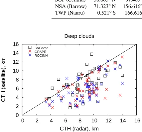
In order to test the soundness of SNGome cloud top height retrievals, we compare the results with ground-based
measurements and with two different and independent space-based algorithms. The ground-space-based data are collected at three different several Atmospheric Radiation Measurement (ARM) climate research facilities (Clothiaux et al., 2000) and at the Chilbolton Facility for Atmospheric and Ra-dio Research (CFARR). The satellite-based retrievals come from the GRAPE (Poulsen et al., 2011; Sayer et al., 2011) dataset made freely available via the British Atmospheric Data Center (http://badc.nerc.ac.uk/data/grape/) and from the Retrieval of Cloud Information using Neural Network (ROCINN, Loyola et al., 2007) dataset, operationally de-ployed by DLR. The basic idea behind this comparison is to gain insight on the strength and weakness of each technique. They rely on three different physical principles: the ARM data are based on active measurements of a millimeter-wave cloud radar, the GRAPE data on the passive thermal mea-surements of ATSR-2 instead, while the ROCINN data are based on the O2 A-band technique in the framework of the
neural network approach. Clearly different parts of the cloud are sensed and the intercomparison is not straightforward. 3.3.1 Satellite- and ground-based data
The Along-Track Scanning Radiometer (ATSR-2) (Stricker et al., 1995) is a dual-view sounder onboard the ESA ERS-2 space platform, being the natural choice for comparison with GOME since no temporal lag between the two instruments and the same cloud scene is assumed. Even so, the limited across-nadir swath (≈500 km) of the ATSR-2 reduces the number of co-registered retrievals of SNGome, resulting in a decreased spatial coverage. The radar facilities description used in this evaluation is given in Table 5.
The physical principle of the GRAPE algorithm is the cloud infrared (IR) brightness temperature as observed by ATSR-2 (Poulsen et al., 2011). Clouds located higher up in atmosphere are generally colder. Local temperature profiles are used to match the derived cloud-top-temperature with the equivalent cloud altitude. The main assumptions in the GRAPE retrieval scheme are: look-up-tables of atmospheric transmittance and reflectance (DISORT as radiative trans-fer code and MODTRAN for the gaseous absorption part); Lambertian surface (MODIS albedo product for 2002); cloud model as a single layer; pressure, temperature and H2O
pro-files according to ECMWF (ERA-40 dataset). More details on the algorithm can be found in Poulsen et al. (2011), while an evaluation of the data, and the criteria for data selection, are given in Sayer et al. (2011). SNGome data selection and properties are as follows: the ground-based site is inside the GOME pixel at a maximum of half of its size; the quality flags are 2 and 5; no restriction on fractional cloud cover has been made. Hence cloud fraction is in the range [0.17–1] for the investigated scenes (i.e. no overcast clouds).
Table 5. Location of the radar facilities with elevation above mean sea level and number of matches for deep and shallow clouds.
Site Latitude Longitude Elevation, m Matches (deep/shallow)
Chibolton 51.145◦N 1.437◦W 90 9/2
SGP (Central) 36.605◦N 97.485◦W 320 28/9
NSA (Barrow) 71.323◦N 156.616◦W 8 12/1
TWP (Nauru) 0.521◦S 166.616◦E 7.1 2/3
0 2 4 6 8 10 12 14 16
0 2 4 6 8 10 12 14 16
CTH (satellite), km
CTH (radar), km Deep clouds
SNGome GRAPE ROCINN
Fig. 5. Comparison between radar ground-based and satellite-based CTH retrievals for deep clouds.
0 2 4 6 8 10 12 14 16
0 2 4 6 8 10 12 14 16
CTH (satellite), km
CTH (radar), km Shallow clouds
SNGome GRAPE ROCINN
Fig. 6. As Fig. 5, but for shallow clouds.
clouds” otherwise. We stress that the “deep” clouds do not refer to the customary deep convective systems, but instead emphasizes the vertical heterogeneous extent of the sensed scene, as it can be seen in Figs. 9 and 10 in Sayer et al. (2011, 3924–3925). This distinction has been made in view of the fact that vertically heterogeneous clouds might occur, in contrast to single-layered homogenous ones, and has been adopted here for consistency with the results given in Sayer et al. (2011).
-3 3
∆
, km
0 2 4 6 8 10 12 14 16 18
CTH, km
SNG ROC Radar
GRAPE
SGP Chib. TWP NSA
0 2 4 6 8 10 12 14 16 18
CTH, km
All sites, shallow clouds
SNG ROC Radar
GRAPE
SGP Chib. TWP NSA
Fig. 7. Upper panel: comparison of retrieved CTH as function of ground-based facility for the shallow cloud case of Fig. 6. Lower panel: CTH bias between SNGome and Radar.
A total 51 co-registered overpasses have been selected for the deep cloud scenario, 15 overpasses have been matched for the shallow cloud scenario and the respective plots are given in Figs. 5 and 6. The statistics are shown in Table 6. First, the findings confirm what has been already explained by Sherwood et al. (2004); Rozanov et al. (2006) and Sayer et al. (2011). Infrared sounding techniques are affected by a systematic bias, as a consequence of the assumption that a cloud is a blackbody radiator in the IR; for that reason the profile matches at higher temperature, placing the cloud too low. This effect can be seen in both cloud field types. Espe-cially for deep clouds the simultaneous retrieval of top and bottom altitude seems to be more suitable, despite the fact that a single layered cloudiness is assumed in the model. It has been shown that inference of both parameters, using the full spectral informations in the A-band (Rozanov et al., 2004) or multi-angular measurements (Ferlay et al., 2010), mitigates this uncertainty. We recall here that, in order to ac-count for the vertical photon penetration depth in GRAPE, a first-order correction was introduced in Sayer et al. (2011) and it resulted in a better (smaller bias) comparison. How-ever this correction was not applied to GRAPE in the present study.
Table 6. Cloud top height (km), correlation coefficientrand aver-age bias (Radar – Satellite, km) for 51 matches of deep (Fig. 5) and 15 matches of shallow (Fig. 6) clouds. The fractional cloud cover for the GOME pixels is in range [0.17–1].
deep (r) shallow (r) Bias (deep/shallow)
Radar 8.51 4.78 –
SNGome 6.89 (0.57) 5.67 (0.75) −1.62/0.89 GRAPE 6.03 (0.52) 4.11 (0.88) −2.48/−0.67 ROCINN 5.72 (0.62) 4.96 (0.69) −2.79/−0.18
Time [hour]
Height [km]
9:00 10:00 11:00 12:00 13:00 14:00 15:00 16:00
15
12
9
6
3
0 −80
−70 −60 −50 −40 −30 −20 −10 0 10 20
[dBZ]
Fig. 8. Millimeter wave cloud radar (MMCR) reflectivity profile of 5 July 2001 at TWP Nauru (see http://www.arm.gov/data/vaps).
frequently westward downwind cloud trails (Henderson et al., 2006), which are, in turn, linked to aerosol produc-tion. It is therefore likely that, on the GOME pixel scale, the assumption of a single-layer cloud is not appropriate. As an example, the radar reflectivity profile for the day 5 July 2001 has been plotted. Given a mean wind speed of 5 m s−1and westward direction, the scene sensed by GOME is highly heterogeneous (see Fig. 8). We see three distinct layers. At the overpass time of GOME, the radar CTH was 7.4 km, this being the intermediate layer. SNGome CTH was 13.02 km (COT 10.26). GRAPE placed the cloud at 4.82 km (COT 2.2), which is the layer of radiative cloud height. Clearly the uppermost layer was retrieved by SNGome, han-dling the space between layers as if it were a single cloud slab.
Overall, where the satellite retrievals deviate from radar top height, they exhibit opposite signs, backing the idea of synergistic use of oxygen A-band and infrared techniques. Therefore, the profiling capabilities of the former together with the radiative sounding of the latter can result in value-added datasets and should not be rejected for future instru-ments’ design.
3.3.2 Satellite-based data
The Retrieval of Cloud Information using Neural Network (ROCINN) algorithm (Loyola, 2004; Loyola et al., 2007)
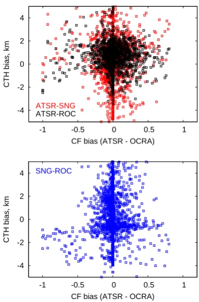
-4 -2 0 2 4
-1 -0.5 0 0.5 1
CTH bias, km
CF bias (ATSR - OCRA) ATSR-SNG
ATSR-ROC
-4 -2 0 2 4
-1 -0.5 0 0.5 1
CTH bias, km
CF bias (ATSR - OCRA)
SNG-ROC
Fig. 9. Scatterplots for CTH bias versus CF bias between IR-based and O2 A-band-based retrievals (upper panel) and the same
be-tween the O2 A-band-based retrievals. Original dataset presented
in Rozanov et al. (2006).
uses the oxygen absorption band and a combination of look-up-tables of forward reflectivities and neural network to de-liver cloud top height (pressure) and albedo, with the same cloud fraction used in SNGome and calculated with OCRA (Optical Cloud Recognition Algorithm, Loyola and Ruppert, 1998; Loyola et al., 2007). We compare the same dataset as described in the work of Rozanov et al. (2006). Four sep-arate GOME orbits (15 453, 16 910, 18 366, 19 537, for a total pixel number of 2422) were selected, which are con-sidered to be representative of climatological and geometri-cal illumination conditions. Such orbits have been operated in enhanced narrow observation mode (i.e. ground pixel size 80×40 km2), thus the results can be extended to instruments with equivalent spatial resolution as GOME-2 (80×40 km2) and SCIAMACHY (30×60 km2).
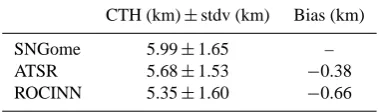
For the large GOME pixel size, an error in cloud fraction impacts the cloud top height retrieval. Assuming the ATSR cloud fraction as the true one (due to the better spatial res-olution), we show in Fig. 9 the CTH bias of the two O2
Table 7. Statistics for average values of all orbits in Rozanov et al. (2006) for three retrieval algorithms. Bias values are given w. r. t. SNGome. Total number of pixels 2422.
CTH (km)±stdv (km) Bias (km)
SNGome 5.99±1.65 –
ATSR 5.68±1.53 −0.38
ROCINN 5.35±1.60 −0.66
cluster in the plot against IR retrievals for both O2A-band
al-gorithms. This is an indirect corroboration of the validity of the independent pixel approximation.
The comparison between SNGome and ROCINN dis-closes a cluster of retrievals where CF underestimation leads to a slight CTH overestimation. This cluster corresponds to the low-level clouds of 2–3 km height of Fig. 10. Being all parameters equal for SNGome and ROCINN, this bias can be explained through the enhancement of radiation backscat-tered to the platform, because of the higher fractional cloud cover. Only in this scenario the assumption of a Lambertian cloud model leads to CTH overestimate, with respect to a model where multiple scattering is taken into account.
Overall, ROCINN tends to underestimate CTHs with re-spect to SNGome (in Table 7 the statistics of the four or-bits are given). A negative bias of−0.63±1.46 km (Loy-ola et al., 2007) and, more recently, of−0.44 km±1.26 km (Loyola et al., 2010) have been found, where the same record of CTHs from GOME and METEOSAT were com-pared. The difference likely arises from the assumption in the ROCINN forward model that a cloud is a perfect Lam-bertian reflector, hence not accounting for multiple scatter-ing of light inside the cloud. Scatterplots between the three CTH products for the 4 orbits are given in Fig. 10. In general, SNGome shows high correlations with both ATSR (0.81) and ROCINN (0.86). ROCINN itself exhibits an excellent corre-lation (0.95) with ATSR. We underline that ROCINN algo-rithm is based on a neural network approach, which relies on the beforehand training of its components and offers a lim-ited space of solutions, whereas SNGome makes no assump-tion for the sensed scene. SNGome agrees better with IR re-trievals for low and mid-level (CTH<7 km) clouds than for high-level clouds. The possible reason for such scattered re-trievals likely arise from the presence of ice or mixed-phase clouds, whose unknown phase function (and lower asym-metry parameterg) enhance light scattering in the sideward direction.
4 Results
This section is devoted to the analysis of cloud top height derived from GOME observations during the period from June 1996 through May 2003, due to missing global coverage after June 2003. We consider zonal averages and inter-annual
0 2 4 6 8 10 12 14 16
CTH (SNGome), km
0 2 4 6 8 10 12 14 16
CTH (ATSR), km y=1.09 x+0.01
R=0.81
0 2 4 6 8 10 12 14 16
CTH (SNGome), km
0 2 4 6 8 10 12 14 16 CTH (ROCINN), km
y=1.06 x+0.57 R=0.86
0 2 4 6 8 10 12 14 16
CTH (ROCINN), km
0 2 4 6 8 10 12 14 16 CTH (ATSR), km
y=1.03 x−0.56 R=0.95
Fig. 10. Scatterplots and correlations among the three CTH prod-ucts derived by satellite measurements for four GOME orbits. The original dataset was presented in Rozanov et al. (2006).
4.1 Data selection
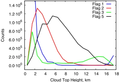
In Fig. 11 we plotted the occurrences of the quality flags (see Table 4 for their meaning) for the complete dataset in func-tion of cloud top height. Accounting for these flags is a cru-cial step for the extraction of realistic cloud scenarios. In this analysis retrievals flagged 0, 1 and 4 are clearly discarded. Specifically, the peak of flag 1 is the consequence of the CTH underestimation introduced by the model (see Fig. 1). For this reason clouds with height<1 km might be underrepre-sented in the record. We make use of retrievals flagged 2, 3 and 5. Data flagged 2 appear as long as the 2-parameter mini-mization of Sect. 2.2 converges only for cloud top height and not for cloud bottom height. In view of the synthetic study presented in Sect. 3.2, we notice that retrievals flagged 3 ap-pear when the upper layer becomes optically thick enough to generate a multi-layer cloud system. The situation con-tributes to the second mode of the green curve of Fig. 11. Thus we will reject such retrievals above a limit height of 5 km.
4.2 Global geographical analysis
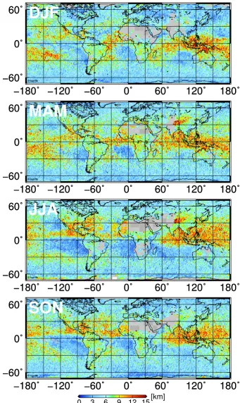
We focus on geographical cloud top height distributions. Our aim is to highlight regional trends and annual distributions. For this purpose, the year 2001 is plotted for the four sea-sons in Fig. 12. The maps have been projected onto a lattice of 0.5◦×0.5◦after a pixel-counted average of daily compos-ites. However, the ungridded retrievals are available as origi-nal data at IUP Bremen website (http://www.iup.uni-bremen. de/∼sciaproc/SNGome/). In fact the main features of global cloudiness are already known and have been studied by other satellite groups (Rossow and Schiffer, 1999; Wylie et al., 2005; Chang and Li, 2005; Stubenrauch et al., 2006; Jensen et al., 2008; Loyola et al., 2010). Nevertheless is it worth to mention that, in the presented maps, some world regions over ocean (and sometimes over portions of the coast) are char-acterized by specific cloud systems. A cloud system may be represented by one or several interacting cloud structures and even with the coarse spatial resolution of the instrument we are able to detect some of them on a global scale.
Namely, over North Atlantic at mid-latitudes the “extra-tropical cyclones” form in the late autumn through winter months and they can reach altitudes of≈9 km. Such cloud systems are detected by SNGome. Especially the seasonal-ity of the monsoon (stretching from South-East Asia to the Arabian Sea) is well pictured, together with the appearance of the typhoons’ cloud structures in the late summer and in the autumn in the far east region bordered by Japan from the north side and Taiwan from the south. The habitual cloud structures termed “marine stratocumulus clouds” can be seen over south Pacific, close to south Peruvian and Chilean coast. Their accumulation is mainly due to the cold Humboldt Sea current, the high mountainous coast and winds from the An-des. They reach 1.5–2 km, rarely exceeding such altituAn-des.
0.0⋅100
2.0⋅105
4.0⋅105
6.0⋅105
8.0⋅105
1.0⋅106
1.2⋅106
1.4⋅106
0 2 4 6 8 10 12 14 16 18
Counts
Cloud Top Height, km Flag 1 Flag 2 Flag 3 Flag 5
Fig. 11. Quality flag counts in function of cloud top height for the 7 yr of the SNGome dataset. The meaning of the flags is given in Table 4.
This region resembles the Benguela region, situated over south Atlantic, where cloud cells formation is mainly due to the cold sea current and the warm winds from the con-tinent. Another feature is the season-conditioned cloudiness over the Caribbean Sea, where hurricanes are observed in the late summer and in the autumn.
In Fig. 13 we present zonally averaged seasonal vertical distributions of relative cloud amount for the year 2001 for the same data in Fig. 12. Data are normalized in a way that for each latitude belt (1.5◦increment) the sum of all CTH oc-currences is equal to 100 %. The seasonality is again well re-produced and the structure of the Intertropical Convergence Zone (ITCZ) with high clouds near the tropopause is de-picted. In Stubenrauch et al. (2010, Fig. 8, p. 7207), datasets from CALIPSO, AIRS-LMD and the radar-lidar GEOPROF are compared for years 2007–2008, boreal winter and sum-mer, and similar plots are presented. Notwithstanding the dif-ferent temporal coverage, we observe a similar shift of the maximum around the equator. This maximum is placed by SNGome at ≈12–13 km: lower than CALIPSO and GEO-PROF and similar to AIRS-LMD. This behavior is expected because, in the case of a thick layer underneath a thin one, SNGome detects the former.
As a further investigation, cloud distributions are analyzed with respect to season, hemisphere and underlying surface. Retrievals are binned with 0.25 km spacing and normalized to the total number of counted cloudy pixels. Additionally we filter cloud fractions smaller than 0.3 in order to screen occasional dust events and to be consistent with the analysis of Joiner et al. (2012). The distributions are plotted in Fig. 14 for year 2001 and the disentanglement of the frequency dis-tributions is plotted in Fig. 15.
−
180˚
−
120˚
−
60˚
0˚
60˚
120˚
180˚
−
60˚
0˚
60˚
−
180˚
−
120˚
−
60˚
0˚
60˚
120˚
180˚
−
60˚
0˚
60˚
0
3
6
9 12 15
[km]
© iup/ife
DJF
−
180˚
−
120˚
−
60˚
0˚
60˚
120˚
180˚
−
60˚
0˚
60˚
−
180˚
−
120˚
−
60˚
0˚
60˚
120˚
180˚
−
60˚
0˚
60˚
0
3
6
9 12 15
[km]
© iup/ife
MAM
−
180˚
−
120˚
−
60˚
0˚
60˚
120˚
180˚
−
60˚
0˚
60˚
−
180˚
−
120˚
−
60˚
0˚
60˚
120˚
180˚
−
60˚
0˚
60˚
0
3
6
9 12 15
[km]
© iup/ife
JJA
−
180˚
−
120˚
−
60˚
0˚
60˚
120˚
180˚
−
60˚
0˚
60˚
−
180˚
−
120˚
−
60˚
0˚
60˚
120˚
180˚
−
60˚
0˚
60˚
0
3
6
9 12 15
[km]
© iup/ife
SON
−180˚
−120˚
−60˚
0˚
60˚
120˚
180˚
−60˚
0˚
60˚
−180˚
−120˚
−60˚
0˚
60˚
120˚
180˚
−60˚
0˚
60˚
0
3
6
9 12 15
[km]
© iup/ife
SON
Fig. 12.Maps of seasonal cloud top height for year 2001 for clouds with optical thickness>5. Top to bottom:
DJF, MAM, JJA, SON.
Fig. 12. Maps of seasonal cloud top height for year 2001 for clouds with optical thickness>5. Top to bottom: DJF, MAM, JJA, SON.
−60˚ −40˚−20˚ 0˚ 20˚ 40˚ 60˚ 2
4 6 8 10 12 14 16
Cloud Top Height, km
DJF
−60˚ −40˚ −20˚ 0˚ 20˚ 40˚ 60˚ 2
4 6 8 10 12 14 16
Cloud Top Height, km
MAM
−60˚ −40˚−20˚ 0˚ 20˚ 40˚ 60˚ 2
4 6 8 10 12 14 16
Cloud Top Height, km
JJA
−60˚ −40˚ −20˚ 0˚ 20˚ 40˚ 60˚ 2
4 6 8 10 12 14 16
Cloud Top Height, km
SON
0 5 10 15
[%]
Fig. 13.Zonally averaged relative amount of seasonal cloud top height for year 2001. Top-left clockwise: DJF,
MAM, JJA, SON.
0 1 2 3 4 5
Frequency, %
0 2 4 6 8 10 12 14 16 18
Cloud Top Height, km PDF for 2001
land water
Fig. 14.Histogram of global cloud top height for 2001.
Fig. 13. Zonally averaged relative amount of seasonal cloud top height for year 2001. Top-left clockwise: DJF, MAM, JJA, SON.
the high peaks in boreal cold seasons have to be linked to austral warmer seasons. In particular, in the Southern Hemi-sphere we find again the hallmark of the persistent low-level cloud structures which contribute to the first modes, as seen in Fig. 15d. It is evident from Figs. 14, 15a and 15c that cloud top heights over land follow a bimodal distribution, whereas in both hemispheres over water appear broader and even tri-modal distributed. Given that averaged global cloud distribu-tions hide short-time fluctuadistribu-tions, we found good agreement with the shape of distributions for July 2007 derived from Cloudsat profiles and presented in Joiner et al. (2012, Fig. 13, p. 540).
4.3 Zonal analysis
Average plots of cloud top height over years minimize the influence of short-time variations. Nevertheless in Fig. 16, during the period 1997–1998, a shift in the maximum can be observed. If one considers cloud height as a proxy for atmosphere dynamics and radiative processes, there might be a link to the development of El Ni˜no-Southern Oscilla-tion (ENSO). In 1997, when the ENSO had its first appear-ance within this record, a single maximum of zonal CTH at
0 1 2 3 4 5
Frequency, %
0 2 4 6 8 10 12 14 16 18
Cloud Top Height, km
PDF for 2001
land water
Fig. 14. Histogram of global cloud top height for 2001.
≈8.8 km was situated in the belt 3◦N–10◦N. As the ENSO developed further, reaching its maximum between November 1997 and April 1998, two distinct maxima of≈8.4–8.5 km each were observed at 3◦S and 10◦N.
0 1 2 3 4 5 6 7
Frequency, %
0 2 4 6 8 10 12 14 16 18
Cloud Top Height, km
Seasonal PDF over land for 2001, north
DJF MAM JJA
SON
(a)
0 1 2 3 4 5 6 7
Frequency, %
0 2 4 6 8 10 12 14 16 18
Cloud Top Height, km
Seasonal PDF over water for 2001, north
DJF
MAM JJA
SON
(b)
0 1 2 3 4 5 6 7
Frequency, %
0 2 4 6 8 10 12 14 16 18 Cloud Top Height, km
Seasonal PDF over land for 2001, south
DJF MAM
JJA
SON
(c)
0 1 2 3 4 5 6 7
Frequency, %
0 2 4 6 8 10 12 14 16 18
Cloud Top Height, km Seasonal PDF over water for 2001, south
DJF MAM JJA
SON
(d)
Fig. 15. Seasonal histograms of cloud top height for 2001. (a) Over land, north; (b) over water, north; (c) over land, south; (d) over wa-ter, south. North = 0–70◦N, south = 0–70◦S.
3 4 5 6 7 8 9 10
-60 -40 -20 0 20 40 60
Cloud Top Height, km
Latitude, degree
1997 1998 1999 2000 2001 2002
Fig. 16. Multiannual average cloud top heights from GOME.
Pacific Ocean. The combination with the longitudinal Walker circulation and Earth rotation had the net effect to strengthen convection loops along the equator and to change heat distri-bution maps at the surface.
Cloud cover trends, retrieved in the O2A-band, have been
found to be positively correlated with sea surface tempera-ture (SST) (Wagner et al., 2005). Moreover, SST anomalies over Pacific Ocean have been found to be negatively corre-lated with O2absorption (Wagner et al., 2008). Thus an
in-crease in SST implies a shallower O2 band, that is higher
CTHs. This effect could be observed in ISCCP records dur-ing the ENSO episode back in 1987–1988: a change of SST of 2◦C for temperatures>26◦C lowered cloud top pressure of≈25 hpa (Bony et al., 1997), which means an increment in CTH of≈0.6 km, therefore matching our retrievals when the maxima of 1997 and 1998 at 3–5◦S are compared.
More recently, Larson and Hartmann (2003) numerically probed the response of tropical clouds and water vapor to SST anomaly. Their findings suggest that high cloud occur-rence rises as compared to middle or low cloud ones. We focus on the tropical pacific region (7.5◦S–10◦N, 100◦E– 280◦E), as specified in Cess et al. (2001). High clouds (HC) are defined as clouds withh >6.5 km, middle clouds (MC) with 3.2 km< h <6.5 km and low clouds (LC) with
h <3.2 km (Stubenrauch et al., 2010); in Fig. 17 their monthly relative averages are plotted. The seasonality, more pronounced in the HC, starting from mid 1998 onward un-til December 2002, is broken during the ENSO anomaly. In the time window February 1997–September 1998, the high cloud abundance never drops below 65%, and middle and low cloud do not exhibit any periodicity either. This confirms the role enhanced convection plays, linking the oceanic cou-pled system of dispersive Kelvin and off-equatorial non-dispersive Rossby waves (Dijkstra, Jan. 2002) with clouds in the tropics.
0 20 40 60 80 100
1997 1998 1999 2000 2001 2002 2003
Frequency, %
Year
Pacific Region (7.5°S − 10°N, 100°E − 280°E)
LC/C MC/C HC/C
Fig. 17.Average relative cloud amount for low (LC), middle (MC) and high (HC) clouds in the Pacific Region where the El Ni˜no anomaly (1997–1998) has been observed.
-4 0 4
-60 -40 -20 0 20 40 60
∆
, km
Latitude, degree 4
5 6 7 8 9 10
Cloud Top Height, km
DJF JJA
Fig. 18. Upper part of the plot: multiannual average of cloud top height in boreal winter (DJF) and boreal summer (JJA). Lower part of the plot: difference JJA - DJF.
37
Fig. 17. Average relative cloud amount for low (LC), middle (MC) and high (HC) clouds in the Pacific Region where the El Ni˜no anomaly (1997–1998) has been observed.
-4 0 4
-60 -40 -20 0 20 40 60
∆
, km
Latitude, degree 4
5 6 7 8 9 10
Cloud Top Height, km
DJF JJA
Fig. 18. Upper part of the plot: multiannual average of cloud top height in boreal winter (DJF) and boreal summer (JJA). Lower part of the plot: difference JJA–DJF.
boreal winter and summer (upper panel) with its difference (lower panel) in Fig. 18. Qualitatively, the CTH maximum is located in ITCZ region centered at 5◦N–10◦N in summer, while in winter the ITCZ moves southward, displacing the maximum at 5◦S–7.5◦S. In terms of hemispheric averages, winters clearly exhibit a lower CTHs at 22◦N–25◦N in the boreal belt, whereas 16◦S–20◦S in the austral belt. In op-posite seasons (i.e. summer), this minimum vanishes and the average CTHs increase. These changes are related to changes in the atmospheric circulation over the annual cycle, that is, in the tropical Hadley cell and mid-latitude Ferrel cells and their intervening ITCZ (Mokhov and Schlesinger, 1993), as shown in the sinusoid in the lower panel of Fig. 18. For polar regions, the anomalous high peak during the austral winter can be related to a missing snow/ice screening in the algo-rithm. In the case of clouds occurring over bright surfaces, due to missing contrast, the sensitivity to COT retrieval de-creases (Pincus et al., 1995; Kokhanovsky et al., 2003) and the retrieved total optical thickness (typically greater than
0 2 4 6 8 10 12
-60 -40 -20 0 20 40 60
Cloud Top Height, km
Latitude, degree Zonal means (06/1996-05/2003)
SNGome ROCINN
0 10 20 30 40 50
-60 -40 -20 0 20 40 60
Cloud Optical Thickness
Latitude, degree Zonal means (06/1996-05/2003)
SNGome ROCINN
0 0.2 0.4 0.6 0.8 1
-60 -40 -20 0 20 40 60
Cloud Albedo
Latitude, degree Zonal means (06/1996-05/2003)
SNGome ROCINN
Fig. 19. Multiannual averaged zonal cloud top height (top panel), cloud optical thickness (mid panel), cloud albedo (bottom panel) and 2σ confidence interval from SNGome and ROCINN.
100) will be the sum of snow OT plus cloud OT. Similar to the two-layer system presented in Sect. 3.2, the retrieved CTH will be biased high.
CTH and COT can be explained as follows. CTH depends, to a certain extent, on the COT values, because the depth of the O2A-band around 760 nm changes in function of COT (see
Fig. 8 in Kokhanovsky and Rozanov, 2004, p. 46). There-fore if the independent piece of information of actual COT values is not used as input for the forward radiative transfer calculations along the band, the resulting CTH can be biased low.
In general, the high values of CA calculated by SNGome can be understood in this way: the asymptotic relations used in this work hold only for clouds withτ >5, therefore thin-ner clouds do not contribute to the global statistics. Another limitation is the GOME spatial resolution. Horizontal and vertical variability of clouds can introduce systematic bi-ases in cloud albedo (Pincus et al., 1999; Oreopoulos et al., 2007). A heterogeneous cloud, which is likely to be sensed by GOME, has always a lower albedo than its homogeneous counterpart, both having the same optical thickness. Thus, treating real clouds as plane-parallel slabs leads to higher albedos. On the other hand, we speculate that a positive trend in aerosol optical thickness (AOT) over ocean, as reported by Thomas et al. (2010, Table 4, p. 4861), impacts cloud albedo through a decrease in mean cloud droplet radius. This effect has been already seen for weak volcanic eruptions over ocean (Gass´o, 2008). The negative correlations shown in Bulgin et al. (2008) between aerosol optical thickness and effective radius corroborate also this hypothesis. However, these re-sults pertain only to oceanic regions, which are affected by continental aerosol outflows. Note that the AOT signals in Bulgin et al. (2008) and Thomas et al. (2010) are derived from ATSR-2 measurements, therefore temporal and spatial co-registration with GOME are not an issue.
Overall the global average cloud top height, derived from GOME measurements for the period June 1996–May 2003, is 5.6±3.2 km in the belt of ±70◦ latitude, for a corre-sponding average cloud optical thickness of 19.1±13.9 and average cloud albedo of 0.63±0.10. We underline that the given average cloud top height is not weighted by the spective average cloud optical thickness. The overview of re-gional statistics of the retrieved cloud properties is given in Table 8.
5 Conclusions
We have presented properties of a seven-year global cloud dataset (see http://www.iup.uni-bremen.de/∼sciaproc/ SNGome/) from the Global Ozone Monitoring Experi-ment GOME using the semi-analytical cloud retrieval algo-rithm SACURA, hereafter termed SNGome. The retrieval is based on optimal estimation approach applied to radiances around the 760 nm O2 absorption A-band. Auxiliary data
used in the calculation are the minimum Lambert-equivalent reflectivity values from TEMIS and the cloud cover from OCRA-DLR, both derived from GOME measurements. The
Table 8. Zonal average values and standard deviations (1σ) of Cloud Top Height (CTH), Cloud Optical Thickness (COT) and spherical Cloud Albedo (CA) derived from GOME measurements from June 1996 to May 2003.Nis the number (in millions) of ob-servations used in the statistics.
Region CTH (km) COT CA N
60◦N–70◦N 4.51±2.19 22.2±16.9 0.65±0.11 0.95 35◦N–60◦N 5.31±2.74 20.4±15.1 0.64±0.11 2.79 15◦N–35◦N 6.66±3.66 18.3±13.3 0.62±0.10 1.15 0◦–15◦N 8.41±3.80 18.3±12.9 0.63±0.10 1.07 0◦–15◦S 7.47±3.96 17.2±11.9 0.62±0.09 0.96 15◦S–35◦S 5.88±3.53 15.3±10.9 0.59±0.09 1.60 35◦S–60◦S 4.88±2.64 18.8±13.6 0.63±0.10 4.13 60◦S–70◦S 4.02±2.01 23.8±17.6 0.67±0.12 0.99
Acknowledgements. D. Loyola and DLR are acknowledged for providing the GOME raw radiances and the GDP extraction software. H. Bovensmann and S. No¨el are thanked for their support in understanding instrument’s radiometric issues. The authors thank the two anonymous reviewers, J. Joiner, A. Vasilkov and P. K. Barthia for their help in improving the manuscript. Generic Mapping Tools (GMT, Wessel and Smith, 1998) were used for this work.
Edited by: J. Cermak
References
Bony, S., Lau, K.-M., and Sud, Y. C.: Sea surface temperature and large-scale circulation influences on tropical greenhouse effect and cloud radiative forcing, J. Climate, 10, 2055–2077, doi:10.1175/1520-0442(1997)010<2055:SSTALS>2.0.CO;2, 1997.
Bovensmann, H., Burrows, J. P., Buchwitz, M., Frerick, J., No¨el, S., Rozanov, V. V., Chance, K. V., and Goede, A. P. H.: SCIAMACHY: Mission objectives and measure-ment modes, J. Atmos. Sci., 56, 127–150, doi:10.1175/1520-0469(1999)056<0127:SMOAMM>2.0.CO;2, 1999.
Br¨uhl, C. and Crutzen, P. J.: MPIC two-dimensional model, in: The atmospheric effect of stratospheric aircraft, edited by: Prather, M. and Remsberg, E., NASA Ref. Publications, 103–104, 1993. Buchwitz, M., Rozanov, V. V., and Burrows, J. P.: A correlated-k
distribution scheme for overlapping gases suitable for retrieval of atmospheric constituents from moderate resolution radiance measurements in the visible/near-infrared spectral region, J. Geophys. Res., 105, 15247–15262, doi:10.1029/2000JD900171, 2000.
Bulgin, C. E., Palmer, P. I., Thomas, G. E., Arnold, C. P. G., Camp-many, E., Carboni, E., Grainger, R. G., Poulsen, C. A., Siddans, R., and Lawrence, B. N.: Regional and seasonal variations of the Twomey indirect effect as observed by the ATSR-2 satellite in-strument, Geophys. Res. Lett., 35, doi:10.1029/2007GL031394, 2008.
Burrows, J. P., Weber, M., Buchwitz, M., Rozanov, V. V., Lad-stt¨atter Weissenmayer, A., Richter, A., DeBeek, R., Hoogen, R., Bramstedt, K., Eichmann, K. U., Eisinger, M., and Perner, D.: The Global Ozone Monitoring Experiment (GOME): Mission Concept and First Scientific Results, J. Atmos. Sci., 56, 151–175, doi:10.1175/1520-0469, 1999.
Burrows, J. P., Borrel, P., and Platt, U.: The remote sensing of tro-pospheric composition from space, Springer, Berlin, Heidelberg, doi:10.1007/978-3-642-14791-3, 2011.
Cess, R., Zhang, M., Wang, P., and Wielicki, B.: Cloud structure anomalies over the tropical Pacific during the 1997/98 El Ni˜no, Geophys. Res. Lett., 28, 4547–4550, doi:10.1029/2001GL013750, 2001.
Chang, F.-L. and Li, Z.: A Near-Global Climatology of Single-Layer and Overlapped Clouds and Their Optical Properties Re-trieved from Terra/MODIS Data Using a New Algorithm, J. Cli-mate, 18, 4752–4771, doi:10.1175/JCLI3553.1, 2005.
Clothiaux, E. E., Ackerman, T. P., Mace, G. G., Moran, K. P., Marchand, R. T., Miller, M. A., and Martner, B. E.: Ob-jective determination of cloud heights and radar reflectivities using a combination of active remote sensors at the ARM
CART sites, J. Appl. Meteor., 39, 645–665, doi:10.1175/1520-0450(2000)039<0645:ODOCHA>2.0.CO;2, 2000.
Coldewey-Egbers, M., Weber, M., Lamsal, L. N., de Beek, R., Buchwitz, M., and Burrows, J. P.: Total ozone retrieval from GOME UV spectral data using the weighting function DOAS approach, Atmos. Chem. Phys., 5, 1015–1025, doi:10.5194/acp-5-1015-2005, 2005.
Deirmendjian, D.: Electromagnetic scattering on spherical polydis-persions, Elsevier Scientific Publishing, New York, NY, 1969. Dijkstra, H. A.: Fluid Dynamics of El Ni˜no
Vari-ability, Ann. Rev. Fluid. Mech., 34, 531–558, doi:10.1146/annurev.fluid.34.090501.144936, January 2002. Diner, D. J., Bruegge, C. J., Martonchik, J. V., Ackerman, T. P.,
Davies, R., Gerstl, S. A. W., Gordon, H. R., Sellers, P. J., Clark, J., Daniels, J. A., Danielson, E. D., Duval, V. G., Klaasen, K. P., Lilienthal, G. W., Nakamoto, D. I., Pagano, R. J., and Reilly, T. H.: MISR: A multiangle imaging spectroradiometer for geo-physical and climatological research from Eos, IEEE T. Geosci. Remote, 27, 200–214, doi:10.1109/36.20299, 1989.
Earth Resources Observation and Science (EROS, USGS) Center: The Shuttle Radar Topography Mission (SRTM), http://www. dgadv.com/srtm30/ (last access: October 2009), 2000.
Ferlay, N., Thieuleux, F., Cornet, C., Davis, A. B., Dubuis-son, P., Ducos, F., Parol, F., Ri´edi, J., and Vanbauce, C.: Toward new inferences about cloud structures from multi-directional measurements in the oxygen A band: middle-of-cloud pressure and middle-of-cloud geometrical thickness from POLDER-3/PARASOL, J. Appl. Meteorol. Clim., 49, 2492–2507, doi:10.1175/2010JAMC2550.1, 2010.
Fischer, J. and Grassl, H.: Detection of cloud-top height from re-flected radiances within the oxygen A band, part 1: Theoretical studies, J. Appl. Meteorol., 30, 1245–1259, doi:10.1175/1520-0450(1991)030<1245:DOCTHF>2.0.CO;2, 1991.
Gass´o, S.: Satellite observations of the impact of weak volcanic activity on marine clouds, J. Geophys. Res., 113, D14S19, doi:10.1029/2007JD009106, 2008.
Gottwald, M. and Bovensmann, H.: SCIAMACHY exploring the changing earth’s atmosphere, Springer, Dordrecht, 2010. Heintzenberg, J. and Charlson, R. J. (Eds.): Clouds in the perturbed
climate system: their relationship to energy balance, atmospheric dynamics, and precipitation, Str¨ungmann Forum Reports, MIT Press, Cambridge, Mass., 2009.
Henderson, B. G., Chylek, P., Porch, W. M., and Dubey, M. K.: Satellite remote sensing of aerosols generated by the Island of Nauru, J. Geophys. Res., 111, D22209, doi:10.1029/2005JD006850, 2006.
Jacobowitz, H., Stowe, L. L., Ohring, G., Heidinger, A., Knapp, K., and Nalli, N. R.: The Advanced Very High Resolution Ra-diometer Pathfinder Atmosphere (PATMOS) Climate Dataset: A Resource for Climate Research, B. Am. Meteorol. Soc., 84, 785– 793, doi:10.1175/BAMS-84-6-785, 2003.
Jensen, M., Vogelmann, A., Collins, W., Zhang, G., and Luke, E.: Investigation of Regional and Seasonal Variations in Marine Boundary Layer Cloud Properties from MODIS Observations, J. Climate, 21, 4955–4973, doi:10.1175/2008JCLI1974.1, 2008. Joiner, J., Vasilkov, A. P., Gupta, P., Bhartia, P. K., Veefkind, P.,
doi:10.5194/amt-5-529-2012, 2012.
King, M. D.: Determination of the scaled optical thick-ness of clouds from reflected solar radiation measure-ments, J. Atmos. Sci., 44, 1734–1751, doi:10.1175/1520-0469(1987)044<1734:DOTSOT>2.0.CO;2, 1987.
Kneizys, F. X., Robertson, D. C., Abreu, L. W., Acharya, P., Ander-son, G. P., Rothman, L. S., Chetwynd, J. H., Selby, J. E. A., Shet-tle, E. P., Gallery, W. O., Berk, A., Clough, S. A., and Bernstein, L. S.: The MODTRAN 2/3 report and LOWTRAN 7 model, con-tract F19628-91-C-0132 with Ontar Corp., Philips Lab., Geo-phys. Dir., Hancom AFB, Mass., 261 pp., 1996.
Koelemeijer, R. B. A., Stammes, P., Hovenier, J. W., and de Haan, J. F.: A fast method for retrieval of cloud parameters us-ing oxygen A band measurements from the Global Ozone Monitoring Experiment, J. Geophys. Res., 106, 3475–3490, doi:10.1029/2000JD900657, 2001.
Koelemeijer, R. B. A., de Haan, J. F., and Stammes, P.: A database of spectral surface reflectivity in the range 335–772 nm derived from 5.5 years of 0.5 observations, http://www.temis.nl/data/ler. html, J. Geophys. Res., 108, 4070, doi:10.1029/2002JD002429, 2003.
Kokhanovsky, A. A.: Cloud Optics, Springer, Dordrecht, 2006. Kokhanovsky, A. A. and Nauss, T.: Reflection and transmission of
solar light by clouds: asymptotic theory, Atmos. Chem. Phys., 6, 5537–5545, doi:10.5194/acp-6-5537-2006, 2006.
Kokhanovsky, A. A. and Rozanov, V. V.: The physical parameteri-zation of the top-of-atmosphere reflection function for a cloudy atmosphere–underlying surface system: the oxygen A-band case study, J. Quant. Spectrosc. Ra., 85, 35–55, doi:10.1016/S0022-4073(03)00193-6, 2004.
Kokhanovsky, A. A., Rozanov, V. V., Zege, E. P., Bovensmann, H., and Burrows, J. P.: A semianalytical cloud retrieval algorithm us-ing backscattered radiation in 0.4–2.4 µm spectral region, J. Geo-phys. Res., 108, 4008, doi:10.1029/2001JD001543, 2003. Kokhanovsky, A. A., Mayer, B., Rozanov, V. V., Wapler, K.,
Bur-rows, J. P., and Schumann, U.: The influence of broken cloudi-ness on cloud top height retrievals using nadir observations of backscattered solar radiation in the oxygen A-band, J. Quant. Spectrosc. Ra., 103, 460–477, doi:10.1016/j.jqsrt.2006.06.003, 2007a.
Kokhanovsky, A., Mayer, B., von Hoyningen-Huene, W., Schmidt, S., and Pilewskie, P.: Retrieval of cloud spherical albedo from top-of-atmosphere reflectance measurements performed at a sin-gle observation ansin-gle, Atmos. Chem. Phys., 7, 3633–3637, doi:10.5194/acp-7-3633-2007, 2007b.
Kokhanovsky, A. A., Nauss, T., Schreier, M., von Hoyningen-Huene, W., and Burrows, J. P.: The intercomparison of cloud parameters derived using multiple satellite instruments, IEEE T. Geosci. Remote, 45, 195–200, doi:10.1109/TGRS.2006.885019, 2007c.
Kokhanovsky, A. A., Vountas, M., Rozanov, V. V., Lotz, W., Bovensmann, H., and Burrows, J. P.: Global cloud top height and thermodynamic phase distributions as obtained by SCIA-MACHY on ENVISAT, Int. J. Remote Sens., 28, 4499–4507, doi:10.1080/01431160701250366, 2007d.
Kokhanovsky, A. A., Platnick, S., and King, M. D.: Remote sens-ing of terrestrial clouds from space ussens-ing backscattersens-ing and thermal emission techniques, in: The remote sensing of tropo-spheric composition from space, edited by: Guzzi, R., Imboden,
D., Lanzerotti, L. J., Burrows, J. P., Borrell, P., and Platt, U., Physics of Earth and Space Environments, Springer, Berlin, Hei-delberg, doi:10.1007/978-3-642-14791-3 5, 231–257, 2011. Kuji, M. and Nakajima, T.: Retrieval of cloud geometrical
parame-ters using remote sensing data, in: 11th Conf. on cloud physics, Am. Meteorol. Soc., Ogden, UT, p. JP1.7, 2002.
Kuze, A. and Chance, K. V.: Analysis of cloud top height and cloud coverage from satellites using the O2A and B bands, J. Geophys.
Res., 99, 14481–14491, doi:10.1029/94JD01152, 1994. Larson, K. and Hartmann, D. L.: Interactions among cloud,
wa-ter vapor, radiation, and large-scale circulation in the tropi-cal climate, Part I: sensitivity to uniform sea surface temper-ature changes, J. Climate, 16, 1425–1440, doi:10.1175/1520-0442(2003)016<1425:IACWVR>2.0.CO;2, 2003.
Lelli, L., Kokhanovsky, A. A., Rozanov, V. V., and Bur-rows, J. P.: Radiative transfer in the oxygen A-band and its application to cloud remote sensing, Atti Acc. Pel. Per. (AAPP), 89, C1V89S1P056-1–C1V89S1P056-4, doi:10.1478/C1V89S1P056, 2011.
Loyola, D. G.: Automatic cloud analysis from polar-orbiting satellites using neural network and data fu-sion techniques, IEEE T. Geosci. Remote, 4, 2530–2534, doi:10.1109/IGARSS.2004.1369811, 2004.
Loyola, D. G. and Ruppert, T.: A new PMD cloud-recognition algo-rithm for GOME, ESA Earth Observation Quarterly, 58, 45–47, 1998.
Loyola, D. G., Werner, T., Yakov, L., Thomas, R., Peter, A., and Rainer, H.: Cloud Properties Derived From GOME/ERS-2 Backscatter Data for Trace Gas Retrieval, IEEE T. Geosci. Re-mote, 49, 2747–2758, doi:10.1109/TGRS.2007.901043, 2007. Loyola, D. G., Thomas, W., Spurr, R., and Mayer, B.: Global
pat-terns in daytime cloud properties derived from GOME backscat-ter UV-VIS measurements, Int. J. Remote Sens., 31, 4295–4318, doi:10.1080/01431160903246741, 2010.
Marshak, A., Davis, A., Wiscombe, W., and Titov, G.: The verisimilitude of the independent pixel approximation used in cloud remote sensing, Remote Sens. Environ., 52, 72–78, doi:10.1016/0034-4257(95)00016-T, 1995.
Meijer, Y. J., Swart, D. P. J., Baier, F., Bhartia, P. K., Bodeker, G. E., Casadio, S., Chance, K., Del Frate, F., Erbertseder, T., Felder, M. D., Flynn, L. E., Godin-Beekmann, S., Hansen, G., Hasekamp, O. P., Kaifel, A., Kelder, H. M., Kerridge, B. J., Lambert, J. C., Landgraf, J., Latter, B., Liu, X., McDermid, I. S., Pachepsky, Y., Rozanov, V. V., Siddans, R., Tellmann, S., van der A, R. J., van Oss, R. F., Weber, M., and Zehner, C.: Eval-uation of Global Ozone Monitoring Experiment (GOME) ozone profiles from nine different algorithms, J. Geophys. Res., 111, D21306, doi:10.1029/2005JD006778, 2006.
Menzel, W. P., Frey, R. A., Zhang, H., Wylie, D. P., Moeller, C. C., Holz, R. E., Maddux, B., Baum, B. A., Strabala, K. I., and Gum-ley, L. E.: MODIS global cloud-top pressure and amount estima-tion: algorithm description and results, J. Appl. Meteorol. Clim., 47, 1175–1198, doi:10.1175/2007JAMC1705.1, 2008.
Moroney, C., Davies, R., and Muller, J. P.: Operational retrieval of cloud-top heights using MISR data, IEEE T. Geosci. Remote, 40, 1532–1540, doi:10.1109/TGRS.2002.801150, 2002.
Nauss, T., Kokhanovsky, A., Nakajima, T., Reudenbach, C., and Bendix, J.: The intercomparison of selected cloud retrieval algorithms, Atmos. Res., 78, 46–78, doi:10.1016/j.atmosres.2005.02.005, 2005.
Oreopoulos, L., Cahalan, R. F., and Platnick, S.: The plane-parallel albedo bias of liquid clouds from MODIS observations, J. Cli-mate, 20, 5114–5125, doi:10.1175/JCLI4305.1, 2007.
Pincus, R., Szczodrak, M., Gu, J., and Austin, P.: Uncertainty in Cloud Optical Depth Estimates Made from Satellite Radiance Measurements, J. Climate, 8, 1453–1462, doi:10.1175/1520-0442(1995)008<1453:UICODE>2.0.CO;2, 1995.
Pincus, R., McFarlane, S. A., and Klein, S. A.: Albedo bias and the horizontal variability of clouds in subtropical marine boundary layers: Observations from ships and satellites, J. Ge