www.the-cryosphere.net/8/25/2014/ doi:10.5194/tc-8-25-2014
© Author(s) 2014. CC Attribution 3.0 License.
The Cryosphere
A wavelet melt detection algorithm applied to enhanced-resolution
scatterometer data over Antarctica (2000–2009)
N. Steiner and M. Tedesco
The City College of New York at the City University of New York, New York, USA Correspondence to: N. Steiner ([email protected])
Received: 4 May 2013 – Published in The Cryosphere Discuss.: 14 June 2013
Revised: 11 November 2013 – Accepted: 13 November 2013 – Published: 7 January 2014
Abstract. Melting is mapped over Antarctica at a high
spa-tial resolution using a novel melt detection algorithm based on wavelets and multiscale analysis. The method is applied to Ku-band (13.4 GHz) normalized backscattering measured by SeaWinds onboard the satellite QuikSCAT and spatially enhanced on a 5 km grid over the operational life of the sensor (1999–2009). Wavelet-based estimates of melt spa-tial extent and duration are compared with those obtained by means of threshold-based detection methods, where melt-ing is detected when the measured backscattermelt-ing is 3 dB below the preceding winter mean value. Results from both methods are assessed by means of automatic weather sta-tion (AWS) air surface temperature records. The yearly melt-ing index, the product of melted area and meltmelt-ing duration, found using a fixed threshold and wavelet-based melt algo-rithm are found to have a relative difference within 7 % for all years. Most of the difference between melting records deter-mined from QuikSCAT is related to short-duration backscat-ter changes identified as melting using the threshold method-ology but not the wavelet-based method. The ability to clas-sify melting based on relative persistence is a critical aspect of the wavelet-based algorithm. Compared with AWS air-temperature records, both methods show a relative agreement to within 10 % based on estimated melt conditions, although the fixed threshold generally finds a greater agreement with AWS. Melting maps obtained with the wavelet-based ap-proach are also compared with those obtained from space-borne brightness temperatures recorded by the Special Sen-sor Microwave/Image (SSM/I). With respect to passive mi-crowave records, we find a higher degree of agreement (9 % relative difference) for the melting index using the wavelet-based approach than threshold-wavelet-based methods (11 % relative difference).
1 Introduction
The future response of the Antarctic Ice Sheet to a changing climate is one of the largest uncertainties in the estimates and predictions of global sea-level rise over the coming decades (Hughes, 1981; Joughin and Alley, 2011; Overpeck et al., 2006; Shepherd and Wingham, 2007; Bromwich and Nicolas, 2010; Dowdeswell, 2006; Lemke et al., 2007). As temperature increases at high latitudes (e.g., Comiso, 2010; Hansen et al., 2010) the rate of surface melting is expected to increase (Ohmura, 2001). Analysis of long-term trends in weather station air temperatures indicates a strongly positive trend in the duration of melting conditions over the Antarc-tic Peninsula (Vaughn, 2006; Barrand et al., 2013). Efforts to quantify mass balance indicate a positive trend in mass loss for much of the West Antarctic Ice Sheet and the Antarctic Peninsula but a negative trend for much of the East Antarc-tic Ice Sheet (e.g., Chen et al., 2011; Rignot and Thomas, 2002; Shepherd and Wingham, 2007; Rignot et al., 2011). Recent results using a combined climate modeling and satel-lite observational approach suggest that in the period 1992 through 2011, the East Antarctic Ice Sheet gains mass at a rate of 14±43 Gt yr−1, while the West Antarctic Ice Sheet and the Antarctic Peninsula exhibit a mass loss of−65±26, and−20±14 Gt yr−1, respectively (Shepherd et al., 2012).
contributed to the process of disintegration through hydro-fracturing (e.g., MacAyeal et al., 2003; Scambos et al., 2009). Instability caused by ice-shelf loss has been shown to in-crease observed ice flow velocity in related glacial tributaries (Rignot et al., 2004; Scambos et al., 2004; Rott et al., 2011). Melting also drives firn densification and compaction (Hol-land et al., 2011).
Direct measurements of melting are not available from in situ data. Additionally, quantities necessary to fully solve the surface energy balance are often unavailable. Therefore, surface melting is generally estimated from near-surface air temperature measurements performed by automatic weather stations (AWS) when and where available. Such measure-ments are sparse over Antarctica and mostly performed around coastal areas and at low elevations. Moreover, data measured from AWS represent only local conditions and are difficult to extrapolate or estimate melting with at large spa-tial scales without adding biases or increasing uncertainty.
Active and passive microwave spaceborne instruments are used to monitor melting over snow-covered areas due to the insensitivity to atmospheric and illumination conditions and high sensitivity to liquid water (e.g., Abdalati and Steffen, 2001; Ashcraft and Long, 2006; Liu et al., 2005; Mote et al., 1993; Nghiem et al., 2001, 2007; Steffen et al., 2004; Tedesco et al., 2007; Torinesi et al., 2003; Wang et al., 2008). For vegetation-free snow-covered areas, the volume scatter component will be dominant for radar backscatter measure-ments at Ku-band frequencies (Ulaby et al., 1982). Backscat-ter loss due to the presence of liquid waBackscat-ter in snow during melting is responsible for a rapid and considerable decrease in the Ku-band normalized microwave backscatter,σ0, with respect to dry snow conditions. This is because of the in-creased imaginary component in the bulk complex dielectric constant of wet snow relative to dry snow (e.g., Ngheim et al., 2001; Stiles and Ulaby, 1980). This same emissivity change will create near-blackbody emission characteristics for wet snowpacks leading to a marked increase in brightness tem-peratures (Ulaby et al., 1982; Stiles and Ulaby, 1980).
Various melt detection algorithms have been developed and applied to active microwave time series to estimate sea-sonal melt. Often, a threshold value of absolute magnitude signal change either constant or regionally variable is used to detect melt-related changes. (e.g., Ashcraft and Long, 2006; Trusel et al., 2012; Wang et al., 2008; Zwally and Fiegles, 1994). Generally, this threshold value is chosen as an approximation of the expected microwave response during snowmelt with respect to a baseline referring to wintertime dry snow conditions (e.g., Ashcraft and Long, 2006). We re-fer to all methods that consider a constant value threshold in the following as fixed-threshold approaches. In contrast, approaches employing physically based temporally or spa-tially variable threshold values will be referred to as dynamic threshold approaches (Mote and Anderson, 1995; Tedesco, 2009). Algorithms that rely on the intrinsic properties of a measurement within time series have also been applied to
snowmelt detection (Joshi et al., 2001; Liu et al., 2005; Wang and Yu, 2011). These approaches are dynamic in that they are based on the magnitude of relative change within each indi-vidual time series. A dynamic approach assumes that large changes in the microwave region are associated with melting events so that “edges” are created in the backscattering time series. These edges can be identified and used to estimate the timing of melting events. Edge-detection algorithms of this type have been developed using derivative-of-Gaussian, (e.g., Joshi et al., 2001) or multiscale wavelet edge detection (Liu et al., 2005).
Building on previous dynamic melt detection approaches (Joshi et al., 2001; Liu et al., 2005), we introduce a wavelet-based melt detection algorithm wavelet-based on multiscale analysis of wavelet transforms to identify melting events using sin-gularity detection (Mallat and Hwang, 1992). Such method identifies points of substantial transition in backscatter time series using no a priori information. In addition to this, a measure of the signal regularity at the point of transition can classify the transition “type”, which allows the separation of persistent melting events (melting lasting continuously for a certain number of days) from transient or sporadic melting events. Besides the wavelet-based approach, we also consider a fixed-threshold algorithm-derived melting record from the same data set. This fixed-threshold record is to evaluate the wavelet-based method where alternative validation data, such as in situ weather-station measurements, are not available. The fixed-threshold method is performed as in Ashcraft and Long (2006) and Barrand et al. (2013). All results of the current dynamic algorithm are shown relative to this fixed-threshold algorithm approach.
2 Methodology
A general overview of wavelets and the specific methodology applied here is presented in Sect. 2.1. This is followed by a more detailed discussion of the mathematics and examples of wavelet melt detection in Sect. 2.2. An overview of the pro-cessing steps and operation of the melt detection algorithm is presented in Sect. 2.3.
2.1 Melt detection using wavelets
The duration of seasonal melting over Antarctica is esti-mated by means of a wavelet analysis. A wavelet transform unfolds a one-dimensional time series of σ0 into a two-dimensional power spectrum of position and scale (i.e., in-verse frequency). The wavelet transform can evaluate local-ized variability of a backscatter time series using a series of convolutions with a dilating and translating wave-like func-tion (Daubechies, 1992). In this study, we use the wavelet transform as a differential operator, in that it is able to ap-proximate the derivative of a smoothed data series at each time location. Melting and refreezing events will cause large variations inσ0and therefore appear as local maxima or min-ima in the wavelet transform.
Many studies in the natural sciences have used the wavelet transform to detect changes in one-dimensional time series, for example the detection of tropical convection anomalies (Weng and Lau, 1994) and geomagnetic jerks (Alexandrescu et al., 1995). Wavelet analysis methods have also been ap-plied to snowmelt detection: specifically, Liu et al. (2005) apply a wavelet-based methodology to identify large changes in measured brightness temperature values associated with melting events over Antarctica.
We apply an approach similar to Liu et al. (2005), but with several key differences. First, we apply this approach to ac-tive microwave (Ku band, 13.4 GHz) measurements. Addi-tionally, we use no a priori information, such as statistical or physically based thresholding of wavelet coefficients, for any of the pixel locations. Melt and refreezing events are both identified and classified in the framework of singular-ity detection as introduced Mallat and Hwang (1992). Con-tinuous wavelet transforms are used to detect melting events that appear as discontinuous events in the backscatter time series and to eliminate those melting events that are deter-mined to be sporadic in time using multiscale analysis (Mal-lat and Hwang, 1992; Mal(Mal-lat, 1999; Alexandrescu, 1995). This methodology is novel, and to our knowledge, it is the first time that such an approach has been applied to remote sensing of snow and ice.
2.2 Continuous wavelet transform and multiscale analysis
The continuous wavelet transform (CWT) of the seasonal (June of one year through May of the successive year)
backscatter,σ0(t )is defined by the convolution product
W σ0(u, s)= Z +∞
−∞
σ0(t )√1 sψ
t−u
s
dt=
ψs∗σ0
(u) ,(1) whereψis the wavelet function,uis the translation param-eter,sis the scaling factor and∗is the convolution operator (Mallat, 1999). The analyzing wavelet,ψ, is a real-valued, localized zero-mean function with a vanishing integral (e.g., the integral ofψis zero) (Mallat, 1999; Holschneider, 1995). The analyzing wavelet function used in this study is defined using the first derivative of a Gaussian function:
ψ (t )=(−1)nd
nθ (t )
dtn (2)
and θ (t )=√1
2πexp
−t
2
2
, (3)
with ordern=1 (Mallat, 1999).
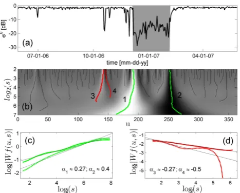
A wavelet function with a Gaussian base is necessary to ensure that wavelet coefficient maxima will be continuous from large to small scales (Mallat, 1999). This allows for the tracing and association of wavelet maxima across scales, a process that is key for multiscale analysis. As an exam-ple, a microwave backscattering time series recorded over the Larsen Ice Shelf AWS during the 2006–2007 season is plotted in Fig. 1a, with the corresponding CWT plotted in Fig. 1b. The magnitude of local maxima or minima inW σ0 (black and white areas, respectively) are correlated with the magnitude of backscatter change (Liu et al., 2005). This is expected asψis equivalent to the first derivative of a smooth-ing function as indicated in Eqs. (2) and (3). In Fig. 1b the conical field of negative W σ0 intercepts the scale axis at its narrowest width at a position (u=185) coincident with a∼20 dB decrease in σ0 over several days. Fields of ele-vatedW σ0in a CWT, or “cones of influence” (Mallat, 1999), are located where the data in the time series (or its deriva-tive) behave as a discontinuous function (Mallat and Hwang, 1992; Holschneider, 1995; Mallat, 1999). Melting or refreez-ing events therefore create cones of influences that will con-verge at fine scales to the position of signal discontinuity (Mallat and Hwang, 1992; Mallat, 1999; Liu et al., 2005). We refer to these positions as singularities (e.g., Mallat and Hwang, 1992).
Fig. 1. (a) QuikSCATσ0time series with the melt duration (MD) estimated using the CWT method shaded in grey. (b) The CWT of the time series in Fig. 1a, where dark-grey to black values indicate positiveW σ0and light-grey to white values negativeW σ0. WT-MMLs are indicated as black, green or red lines associated with melt onset (MO, WTMML 1) melt refreeze (MF, WTMML 2) and sporadic, early season melt (WTMML 3, WTMML 4). (c) TheW σ0
along WTMML plotted over all scales, (s), and the associatedαfor the MO and MF events. (d) Same as Fig. 1c but for an early season sporadic melting.
frequency or scale representation of any signal, is neces-sary in this application as these positions are not easily con-nected if determined only at discrete dyadic scales (e.g., Liu et al., 2005). Additionally, tracing CWT maxima to the finest temporal scale ensures the accurate localization of melting events as these positions will be shifted with increasing scale, as evident in Fig. 1b.
The WTMML is then used to characterize the nature of σ0change at each singularity using multiscale analysis (e.g., Mallat and Zhong, 1992; Le Gondidec et al., 2002). The WTMMLs for several singularities inσ0 are highlighted in Fig. 1b and are labeled 1 through 4. The apparent regularity of aσ0time series in the immediate neighborhood of each singularity can be estimated from the wavelet coefficient val-ues that compose each WTMML (e.g., Mallat, 1999). The Holder exponent, a, is a measure of estimated regularity at the terminating position of each WTMML (Mallat and Zhong, 1992). An estimate ofa is found as (Mallat, 1999)
W σ
0(u, s) ≤Ae
a (4)
so that ln
W σ
0(u, s)
≤alna+lnA. (5)
Here,W σ0
correspond to the wavelet coefficients that com-pose the WTMML. Using Eq. (4) and Eq. (5),a as well as
the coefficientAare determined using a linear least-squares regression.
Each WTMML can be then classified bya using several theoretical transition types whosea value is known. For ex-ample, a step-like or Heaviside function will result in a near 0a(Le Gonidec et al., 2002), while a ramp-like or smoothed transition hasa of 1 or greater (Mallat, 1999; Le Gonidec et al., 2002). For wet snow detection, we assume melt onset transitions (e.g., similar tou=185 in Fig. 1b) can be approx-imated by either a step-like or smoothed transition. Here the corresponding value ofa isa1=0.27. Due to the complex
nature of a time series,avalues determined by Eq. (5) are not expected to match the theoretical case since nearby singular-ities will have contributions to the WTMML (i.e., cones of influence will overlap if transitions are close in time) (Mallat, 1999). In Fig. 1a we observe a more gradual (smoothed)σ0 transition, coincident with a refreezing event nearu=250, where the determined regularity (a2=0.4, Fig. 1c).
Spike-like or cusp-like transitions will produce negative a in multiscale analysis (Le Gonidec et al., 2002; Mallat, 1999). In Fig. 1a, a σ0 fluctuation, corresponding to posi-tion u=140 in Fig. 1b illustrates a transition that is spo-radic in time. This transition produces two WTMMLs, shown in Fig. 1d, labeled 3 and 4, having negative and positive Wσ0 components, respectively. From Eq. (2) it is deter-mined that both can be approximated with negativea values (a3= ∼ −0.27,a4= ∼ −0.4). Negativea values associated
with a WTMML indicate the signal is both discontinuous and non-differentiable at that position, hereu=140 (Mallat and Hwang, 1992). In terms of melt detection, by removing all negativeatransitions, we eliminate sporadicσ0changes that return to “dry” conditions rapidly relative to the reference scale. This creates a melt detection process that eliminates sporadic melting events.
For locations that do not experience melting events, changes in backscatter associated with snow properties changes are of low magnitude compared to changes in liquid water content, but produce positiveain multiscale analysis. To reduce the influence of falsely classified melting events, we set a minimum threshold for |Wσ0|at each temporal scale along the WTMML corresponding to one order of magni-tude (10×) greater than that observed during winter (June, July and August). This is a conservative threshold and this choice does not appear to influence classification for areas experiencing melt.
2.3 Melt detection process
The WTMMLs from each backscattering time series are eval-uated as a possible melting event according to the following criteria:
only at small scales (i.e., high frequency). We set the minimum scale at 25. We observed that using a scale of 23similar to Liu et al. (2005) could not eliminate all noisy transitions during the melting season. This in-creased minimum scale relative to previous studies is expected since the enhanced-resolution remote sensing product used in this study is noisier than the coarser resolution one (Ashcraft and Long, 2006; Spencer et al., 2000).
2. All |Wσ0| along the WTMML must have a value one order of magnitude (10×) greater than those mea-sured during the winter season. For areas experienc-ing melt, this condition does not have a large effect, since |Wσ0| produced at all scales for a∼3 dB transi-tion in backscatter is many orders of magnitude greater than observed wintertime conditions. However, areas that experience snow property changes but no sea-sonal melt will produce WTMMLs with large scalar components since these changes are not “noisy” tran-sitions and are temporally sustained. Since changes in LWC produce greater differences in backscattering values compared to snow property changes over a rel-atively short period (Stiles and Ulaby, 1980), we set the threshold with the |Wσ0| values of a WTMML, at all spatial scales, with a value an order of magnitude (10×) greater than observed wintertime conditions. 3. The Holder exponent, α, of each WTMML must be
equal to or greater than zero. For reasons discussed in the previous section, we eliminate spike-like tran-sitions in backscatter using a test of point-wise signal regularity.
All signal transitions that meet the three criteria above are considered to be either melt onset or refreeze events. To de-fine periods of melt we select the WTMML that extends to the largest scales that has the greatest mean |W σ0|. This tran-sition is matched with a WTMML greatest mean |W σ0| in the set of transitions of opposite magnitude. This defines one seasonal melting event. We assume that refreeze must follow melting. This process is repeated with the remaining melt-related WTMMLs to define additional periods of melting or periods of sustained refreeze within melting. The melt onset (MO) is defined as the first day of melting, and melt-off (MF) is defined as the last melting day plus one. The melt duration (MD) at any pixel location is the total number of days when melting occurs.
A fixed-threshold melting record is created for compari-son, hereafter referred to as FT3. In the FT3 record, melt-ing is classified as where the enhanced-resolution σ0(t) is at or below 3 dB minus winter (June–July–August) mean backscatter, equivalent to the expected backscatter loss from a 2.8 cm layer of 1 % volumetric water content as in Ashcraft and Long (2006). Melting events whose durations are shorter
than three continuous days are removed from the melting record at each pixel following Tedesco et al. (2007).
For our study, we use a MATLAB®wavelet analysis soft-ware library (WaveLab 850) distributed by Stanford Univer-sity and available at http://statweb.stanford.edu/~wavelab/. Because of the computationally intensive nature of the prob-lem and of the high number of pixels necessary to cover the entire Antarctic continent at the spatial resolution considered here (2.225 km), we also made use of the MATLAB’s parallel computing toolbox, running on a dedicated server using eight processing cores. In this configuration, one continent-scale melting season requires between 24 and 48 h of processing.
3 Data sets
3.1 SeaWinds on QuikSCAT
3.2 Automated weather stations
Automated weather station data from the Antarctic Meteo-rological Research Center and Automatic Weather Station program, maintained by the Space Science and Engineer-ing Center at the University of Wisconsin, Madison, are used to evaluate the results of the melt detection algorithms. For our comparison, we use the hand-corrected 3-hourly air tem-perature records. The AWS used in this study are Larsen Ice Shelf (lat. 67.01 S, long. 61.55 W, elev. 17 m), Uranus Glacier (lat. 71.43 S, long. 68.93 W, elev: 780 m), Fossil Bluff (lat. 71.33 S, long. 68.28 W, elev. 63 m), Butler Island (lat. 72.21 S, long. 60.17 W, elev. 91 m), Pegasus South (lat. 77.99 S, long. 166.57 E, elev. 5 m) and Limbert (lat. 75.91 S, long. 59.26 W, elev. 40 m). For each AWS, air-temperature measurements and backscatter are spatially and temporally coregistered using overpass times available from MERS-SCP. Melting is determined from AWS air-temperature mea-surements where there are at least 2–3 h daily above-zero measurements. For Antarctica, extreme fluctuations in daily temperature often prevent the daily mean temperature from exceeding 0◦C, though satellites observations indicate that melting is likely taking place. A threshold below 0◦C is of-ten used to account for this fact (Tedesco and Monaghan, 2009; Van den Broeke et al., 2010), or in those cases where additional measurements are available, such as surface short-wave and long-short-wave radiative fluxes, melting may be de-termined using a simple thermodynamic model (Van den Broeke, 2005). From the lack of a defined sub-zero thresh-old for each AWS station, as well as of sufficient surface measurements for modeling approaches, we choose a tem-poral threshold of at least six hours of above-zero measure-ments in one day to establish melting conditions from AWS measurements and acknowledge that is a source of uncer-tainty in the AWS validation data set. This is equivalent to at least two daily above-zero measurements for the 3 h AWS air temperature data set. Once melt is estimated from AWS data, we study the number of days when the remote-sensing-and air-temperature-based estimates agree (true positive); the omission error, computed as the percentage of days when air temperature indicates melting but the remote sensing-based approach does not (true negative); and the commission, com-puted as the percentage of days when the satellite data indi-cate melting but this is not occurring from the analysis of air temperature (false positive).
4 Results
4.1 Comparison between QuikSCAT-derived melting and analysis of automated weather stations
Results of the FT3 and dynamic wavelet-based (CWT) ap-proaches are compared with estimates of melting derived from surface air temperatures measured by AWS. Because of
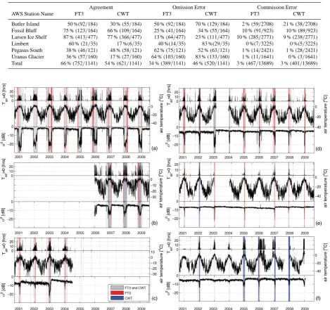
the lack of in situ liquid water content or snow temperature measurements, melt is estimated from AWS air temperatures where the temperature is above zero for at least six hours per day. The time series of coregistered backscattering, air temperature and positive temperatures for the stations con-sidered in this study are plotted in Fig. 2. We evaluate the agreement, commission and omission in percentage at each station, and the results are presented in Table 1. Agreement is defined as the percentage of cases where surface temperature and spaceborne-based estimates both detect melting. Com-mission is defined as the percentage of cases in which re-mote sensing algorithms indicate melting but AWS does not. Lastly, omission indicates the percentage of cases in which AWS suggests melting but the remote sensing algorithms do not.
For stations that experience at least 10 days of melt per year (Butler Island, Fossil Bluff and Larsen Ice Shelf sta-tions), we find the highest rates of agreement. For these stations the FT3 approach performs with more agreement (∼10 %) than the CWT approach. The Larsen Ice Shelf and Fossil Bluff stations show the highest overall agreement, av-eraging 87 % (77 %) and 75 % (66 %) for the FT3 (CWT) approach for all years. Both of these stations have large mag-nitude and sustained change in backscatter over the melting season (Fig. 2a and b). For the Limbert, Butler Island and Uranus Glacier stations, shown in Fig. 2c, d and e, respec-tively, the difference in agreement for the FT3 and CWT methods is greater, up to 43 % (FT3 > CWT) between meth-ods. At these stations, most of the melting occurs as short-duration events. This is not the case during the 2002–2003 and 2003–2004 seasons for the Limbert and Uranus Glacier stations, respectively, where the backscattering time series shows a substantial decrease in backscatter. In this case both remote sensing methods are in good agreement with AWS estimates. Figure 2a and b show that most of the difference between methods at these stations occurs during transitional periods, meaning near the seasonal MO or MF. For the Pe-gasus South station, the CWT method is in better agreement with AWS compared to FT3, with a 10 % greater mean agree-ment. At the Pegasus South station the apparent backscat-ter response to melting, as shown in Fig. 2f, is below de-tection by the FT3. Additionally, the Pegasus South station has the highest mean air temperature during melting condi-tions among these stacondi-tions at+2.16◦C and a mean loss of +1.86 dB (from winter mean) during AWS defined melting. Only the Uranus Glacier station has a smaller backscatter change,+1.80 dB, with an average temperature of+0.79◦C
during melting. In contrast, the Larsen Ice Shelf averages a loss of+15.07 dB with a mean temperature of+1.06◦C dur-ing AWS-defined meltdur-ing.
Table 1. Stations used in the AWS evaluation. Shown are the agreement (true positive), omission (false positive) and commission (true
negative) relative differences from the comparison of melting estimated from AWS air temperatures and melt duration (MD) time series estimated using the FT3 and CWT melt algorithms.
Agreement Omission Error Commission Error
AWS Station Name FT3 CWT FT3 CWT FT3 CWT
Butler Island 50 %(92/184) 30 % (55/184) 50 % (92/184) 70 % (129/184) 2 % (59/2708) 21 % (38/2708)
Fossil Bluff 75 % (123/164) 66 % (109/164) 25 % (41/164) 34 % (55/164) 10 % (91/923) 10 % (89/923)
Larsen Ice Shelf 87 % (413/477) 77 % (366/477) 13 % (64/477) 23 % (111/477) 10 % (285/2771) 9 % (238/2771)
Limbert 60 % (21/35) 17 %(6/35) 40 %(14/35) 83 %(29/35) 0 %(7/3225) 0 %(5/3225)
Pegasus South 38 % (46/121) 48 % (58/121) 62 % (75/121) 52 % (63/121) 1 % (14/2421) 1 % (28/2421)
Uranus Glacier 36 % (57/160) 17 % (27/160) 64 % (103/160) 83 % (133/160) 1 % (11/1641) 0 % (3/1641)
Total 66 % (752/1141) 54 % (621/1141) 34 % (389/1141) 46 % (520/1141) 3 % (467/13689) 3 % (401/13689)
Fig. 2. AWS temperature records for (a) Larsen Ice Shelf, (b), Fossil Bluff, (c), Uranus Glacier, (d) Butler Island, (e) Limbert and (f) Pegasus
South for 2000 to 2009 plotted with the corresponding QuikSCAT backscattering values. Times where the FT3 or CWT approaches estimate melting are shaded red and blue, respectively, while times where both methods agree are shaded grey.
averaging close to 4 days yr−1in length from AWS-derived melting. The majority of these melting events are omitted using the CWT. Conversely, the FT3 approach detects these events with relatively high agreement (83 %). These findings are consistent with the basic principles of the CWT algo-rithm, which aims to detect only sustained melting events. For the Larsen Ice Shelf, we find the lowest rate of omission, averaging 34 % (25 %) for the CWT (FT3). Commission
er-rors are found to be small for both methods, averaging 3 % for all stations for both the FT3 and CWT, respectively.
4.2 Comparison between QuikSCAT melting algorithms
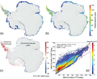
Fig. 3. (a) A map of mean (2000 through 2009) seasonal melt duration estimated from the SeaWinds sensor on QuikSCAT using a 3 dB below
winter mean threshold (FT3) (b) and a continuous wavelet-based method (CWT). (c) The difference between mean MD from both methods is indicated as1MD (FT3-CWT). The location of the Antarctic Peninsula (AP) and Dronning Maud Land (D) are labeled. (d) Autocorrelation analysis using a log-transformed two-axis histogram, where mean MD is compared for all areas where melt is detected by both methods.
MD approaches where1MD=MDFT3−MDCWT. Although
the spatial patterns of MD from the two methods are simi-lar, systematic differences exists regionally and with eleva-tion change. Results are presented and discussed in the con-text of Antarctica as a whole, specific regions and trends in 1MD with elevation.
4.2.1 Continent-scale results
For all areas and years, the CWT algorithm produces an av-erage MD value of 41 days vs. 28 days obtained with the FT3 algorithm. The mean continent-scale melt index (MI), defined as the area subject to melting times the number of melting days, for the two methods is similar although larger for the CWT at 2.971×10⁷day km2than the FT3 at 2.813×10⁷day km2. The MI detected by the CWT is larger than the FT3 because melting events detected by the CWT are continuous and do not contain short-duration intermittent non-melting classifications as in the FT3 melting records. This is also a factor in MD differences; however, the dif-ference in MD can also be explained by the omission of smaller duration melting events by the CWT as shown in air-temperature comparisons at the Butler Island, Uranus Glacier and Limbert AWS. The inclusion of short-duration events in the FT3 record will greatly reduce the mean MD. The total melting extent, defined as the total surface area of Antarctica
subject to at least one day of melting per season, is found to be 6.23 % when using the CWT finds and 8.14 % from the FT3.
The average MO, expressed as day of year, determined by the CWT approach is day 347 (e.g., 13 December for non-leap years) and in the case of the FT3 algorithm is day 352. The mean MF date for the whole of Antarctica be-tween methods differs by 6 days, with the FT3 suggesting a later refreezing (day 28) than the CWT approach (day 22). The difference (5 days MO and 6 days MF) between the seasonal MO and MF obtained with the two approaches is small compared to the standard deviation (σ ) of either method, beingσFT3=26 days andσCWT=16 days for MO
andσFT3=28 days andσCWT=17 in MF over all locations
and years.
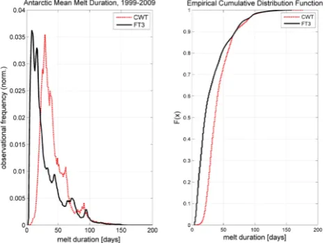
Fig. 4. (a) A histogram of all observed seasonal melt duration in
days for the years 2000 through 2009 for the wavelet-based melt detection method (CWT) and a fixed-threshold method (FT3). It is found that the observations for the CWT are shifted towards longer durations due to the exclusion of short-duration melting events.
(b) An empirical cumulative density function of observed melting
duration.
for MD greater than 34 days, where the CWT method shows longer melt durations.
An analysis of the distribution of melt-duration occur-rences, as shown in Fig. 4a, shows that the CWT algorithm finds more longer MDs relative to the FT3 and that the FT3 is much more likely to detect short-duration events. Close to 5 % of MD values found by the FT3 are 10 days or less, while for the CWT method this accounts for less than 1 % of all detected melting events (Fig. 4b). The inclusion of short-duration melting events using a fixed threshold leads to de-creased mean MD value. The majority (> 50 %) of MDs for the FT3 method are under 27 days, compared to a 37-day MD for the CWT method. Both methods show better agree-ment for longer MD, where about 20 % of all MDs for both methods are 60 days or longer.
4.2.2 Regional results
Detailed results are presented in this section for the Antarctic Peninsula and the coastal area of Dronning Maud Land (as shown in Fig. 3c). These regions are chosen because they exhibit the largest differences in regionally integrated1MD or season length between algorithms.
Over the Antarctic Peninsula, seasonal mean MD val-ues estimated by the CWT and FT3 are similar. The mean MD value obtained from the CWT approach is 55 days and 51 days from the FT3 approach. The spatial distribution of 1MD values obtained with the two approaches (Fig. 3c) in-dicates that the CWT shows generally larger MD values over the ice shelves of the Antarctic Peninsula than those obtained with the FT3 approach. The similarity in mean MD in the
light of a visible difference in MD over large ice shelves can be attributed to the greater melting extent found by the FT3, compared to the CWT, over areas experiencing short melting durations. The melting index over the Antarctic Peninsula is 8.3 % larger for the FT3 than the CWT (the relative differ-ence is defined as|MI1−MI2|
.
1
2(MI1+MI2)).
When observing the seasonal melt initiation over the Antarctic Peninsula, we find that the mean MO date from the FT3 to be day 1 (e.g., 1 January) and the mean MO for the CWT is day 342. The MF dates for the CWT and FT3 over the peninsula are day 46 and day 33, respectively. The FT3 approach estimates a substantially longer (22 days) mean melting season for the Antarctic Peninsula compared to the CWT and most of this difference is due to the estimates of MO.
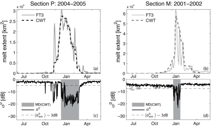
An analysis of selected backscattering time series during the melting season along with regionally integrated melting is presented to show difference between the CWT and FT3 algorithms. For the Antarctic Peninsula during the 2004– 2005 melting season, FT3 values (Fig. 5a, solid grey line) exhibit an early season (November, 2004) peak in ME reach-ing an extent of up to∼80 % of the yearly maximum for a period of∼8 days. This transient melting event is not ob-served in the time series of melting extent from the CWT approach as melt (Fig. 5a, dotted black line). A time series of backscatter from within the region and over this same pe-riod is shown in Fig. 5c. Melting is indicated by a shaded region for the CWT method, and by the location of the 3 dB threshold for the FT3 approach in Fig. 5c, we observe that the CWT excludes several melting events at the beginning of the season (outside of the shaded area) that correspond to the large increase in region-wide melting extent as shown by the FT3 (Fig. 5a). This omission by the CWT here is representative of the differences in melting extent observed regionally. Much of difference between methods over the Peninsula can be attributed to non-sustained short-term melt-ing/refreezing events, as shown in Fig. 5a, before and after the period when most of the melting occurs. Additionally, it is clear that the MO date for most of the Antarctic Peninsula determined using the FT3 approach (defined as the first melt-ing event greater than three days) will correspond to the brief November melting event that, as shown in Fig. 5a, may be several weeks prior to the main melting events. The omis-sions of melting events during transitional periods by the CWT method is also indicated in the AWS validation of the Butler Island, Limbert and Uranus Glacier AWS records.
Fig. 5. (a) A time series of total integrated melt extent for 2004–2005 estimated using the FT3 and CWT methods over the Antarctic Peninsula
(Section P) and (b) during the 2001–2002 melting season for Dronning Maud Land (Section M). Backscattering time series are plotted for
(c) a representative pixel location for the Antarctic Peninsula during the 2004–2005 austral summer and (d) Dronning Maud Land during the
2001–2002 austral summer to illustrate the results of melt classification by of CWT (shaded) and FT3 methods (threshold indicated).
Fig. 6. The empirical probability density function (bar) and
cumu-lative density function (line) of continuous melting periods per sea-son observed over Antarctica (not the total per-pixel seasea-sonal dif-ference) for the 2003–2004 and 2005–2006 season that are found using a FT3 but rejected in by CWT.
found between methods. The percentage of melt days per melting season length (calculated as (MF-MO)/MD) is 65 % for the FT3 method and close to 95 % for the CWT ap-proach. This important difference can be partly attributed to threshold values that underestimate the actual backscat-tering response to increasing liquid water content and as a result backscatter with melting is close in magnitude to the to seasonal in backscatter threshold (e.g., 3 dB). With sig-nal noise, a fixed-threshold algorithm will alternate between classifications of melting and refreeze as backscatter fluc-tuates around the backscatter threshold. Alternatively, sim-ilar fluctuations in backscatter could be attributed to rapid melt–refreeze events in areas where the liquid water content is not sustained through diurnal refreeze cycles. These cases
are difficult to validate without further information and are a weakness of fixed-threshold algorithms in varying snow property and temperature regimes. In the CWT methodology, sustained deviations from wintertime conditions will be de-tected and classified as melt until an additional refreeze tran-sition occurs, regardless of intermittent non-sustained (nega-tivea)fluctuations in backscatter.
A time series of ME and σ0 for Dronning Maud Land are shown in Fig. 5b and d. Here, the CWT method finds a greater regionally integrated MI with respect to the FT3 method. A time series ofσ0 chosen from within Dronning Maud Land, as in Fig. 5c. This backscatter series indicates that the FT3 method will classify multiple melt–refreeze events as σ0 changes rapidly around the threshold value, while the CWT will record a single melting event. This will lead to estimates of a shorter MD by the FT3. It is found that this case is representative of the majority of regions with −1MD. Melting events as shown in Fig. 5d will not result in considerable differences in MO or MF dates.
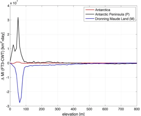
Fig. 7. An analysis of the difference in melting index
(1MI=MIFT3−MICWT)estimates from the FT3 and CWT
meth-ods at a range of elevations for the entire Antarctic continent (red line) as well as the Antarctic Peninsula (black line) and Dronning Maud Land (blue line).
event and CWT does not. During the 2003–2004 season, ∼60 % of MD values differ by only one day,∼20 % show differences of two days, with the remaining values differing by more than six days (∼90 % of observations are six days or less). This six-day duration is similar to the temporal filtering methods used in previous melting studies to eliminate tran-sient melting events (e.g., three days; Tedesco et al., 2007).
4.2.3 Elevation
Figure 7 shows results concerning the difference between the outputs of the two approaches as a function of eleva-tion for the Antarctic Peninsula, Dronning Maud Land and the whole of Antarctica. For the Dronning Maud Land re-gion, the melt index difference between the two methods (1MI=MIFT3−MICWT)is negative, independent of
eleva-tion. For the Antarctic Peninsula, however, the mean differ-ence between methods is positive, and will vary with eleva-tion. For areas below 400 m a.s.l. the CWT method underesti-mates MI with respect to the FT3 method. Conversely, above 400 m a.s.l., the MI difference becomes negative. Building on our previous analysis in this paper, we infer that for the Antarctic Peninsula at lower elevations we find that the melt difference is due to the omission of short-duration melting events, while at higher elevations we find a that melt de-tection differences are more closely related to either short melt–refreeze cycles at high elevations or a lesser backscat-ter response to snow wetness. This may indicate the need for terrain correction when using fixed-threshold methods.
2000 2002 2004 2006 2008
1.5 2 2.5 3 3.5 4 4.5 5 5.5 6 6.5x910
7
year
melt9index9[day
×
km
2]
CWT FT3 MT09 JZ03
0 1 2 3 4 5 6 7
x9107
0 1 2 3 4 5 6 7x910
7
JZ039−9melt9index9[day × km2]
melt9index9[day
×
km
2]
CWT FT3 MT09
(b) (a)
Fig. 8. (a) The time series of total melt index (MI), in day km2, for the Antarctic continent plotted for the years 1999 through 2009 de-rived from the FT3 and CWT methods on an enhanced-resolution QuikSCAT active microwave data set along with estimates from the MT09 and M+K30 methods and an SSM/I data set. (b) The corre-lation between the FT3, QuikSCAT data set MI estimates and the CWT, M+K30 and MT09 methods is indicated using a linear re-gression.
4.3 Comparison with results from passive microwave measurements
We compare melting records from passive microwave SSM/I observations using approaches proposed in the literature with the outputs of both the CWT and FT3 methods. The SSM/I-derived melting is produced using two meth-ods. The first is a fixed-threshold approach as in Zwally and Fiegles (1994), here denoted M+30K. The second data set is produced using a dynamic electromagnetic modeling-based detection approach as in Tedesco (2009), here de-noted MT09. Outputs from both methods are projected onto the 2.225 km QuikSCAT grid using nearest-neighbor inter-polation. Enhanced-resolution passive microwave brightness temperatures generated using the SIR algorithm are available for Antarctica (Long and Stroeve, 2011). Melting records based on these data would reduce scaling discrepancies be-tween the active and passive microwave melt records re-ported here and provide a more consistent analysis. This will be explored in further studies.
The values of seasonally integrated MI for Antarctica for both active and passive microwave methods are plotted in Fig. 8a. The M+30K and CWT approaches show the most similar magnitude in seasonal MI, where the relative differ-ence is 9 %. This is only 2 % greater than the differdiffer-ence be-tween the CWT and FT3 methods (7 %). There is a slightly greater relative difference between the FT3 and M+30K of 11 %. The MT09 method finds on average a 40 % greater MI than the FT3 method, and 35 % greater than the CWT.
season, where most of this difference is from the Antarc-tic Peninsula. Seasonally integrated melting indices derived using the passive microwave methods are well correlated with the QuikSCAT-derived melting records. This relation-ship is shown in Fig. 8b. The best agreement between active and passive microwave records is found between the CWT and M+30K, as indicated in Table 2a. Further, both MT09 and M+30K have a greater degree of correlation and a lower RMSE for the CWT than compared to the FT3.
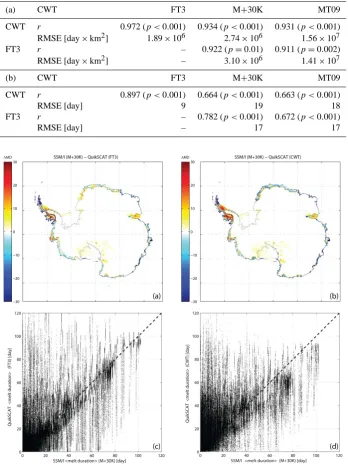
The spatial differences between the mean MD estimated using the M+30K approach and the CWT and FT3 is shown in Fig. 9a and b, respectively. These maps indicate spa-tial patterns in the magnitude of difference between meth-ods (1MDFT3=M+30K-FT3). Over large ice shelves (e.g.,
the Larsen and Amery ice shelves), 1MDFT3 is close to
+10 days (Fig. 9a). Over the same regions, the 1MD be-tween the M+30K and the CWT algorithms is close to +20 days (Fig. 9b). The tendency for the passive microwave data to overestimate active microwave estimates (close to +10 or +201MD in most cases) is usually bordered, to some degree, by an area of underestimation by the passive measurements. The majority of areas that exhibit melting in Antarctica are generally at ice–ocean boundaries. For the Antarctic Peninsula (among other places) areas of melt occur adjacent to sharp contrasts in elevation. For many of these areas sub-pixel mixing will likely lead to a decrease in the observed brightness temperatures of some melting areas. For example, over the coastal regions of Dronning Maud Land we find that the systematic occurrence of positive1MD bor-dered negative1MD. These negative1MDs are found adja-cent to ocean pixels and high elevations and are likely due to a sub-pixel mixing effect. In another case, the relatively nar-row King George VI (lat.−71.965, long.−67.807) Ice Shelf, located roughly east of Wilkens Ice Shelf (lat. −67.525, long.−62.775), appears to increase the apparent MD of the surrounding high-elevation areas for the passive microwave case, resulting in a large positive1MD. Since mixed pixel effects dominate the spatial differences between methods, it is difficult to determine a relationship between MD methods over similar areas other than the positive ∼10 days (FT3) and∼20 days (CWT) reported previously.
An analysis of correlation between colocated melting du-rations from active microwave data sets and the M+30K method indicates that the FT3 has a higher degree of correla-tion with the passive microwave M+30K method Table 2b. It is also found that AMW methods find an RMSE of∼18 days in comparison with both the M+30 and MT09. The rela-tionship between spatially colocated data records are illus-trated the Fig. 9c and d. A first-order least-squares regres-sion between CWT and M+30K shows an∼13-day positive bias. There is an∼3-day positive bias between the FT3 and M+30K from similar analysis. Artifacts that appear as ver-tical striping of data points indicate a high degree of vari-ability for many pixels with similar MD as detected using the M+30K. These are likely a result of a high degree of
sub-pixel variability due to the difference in spatial resolu-tion as previously discussed. In Fig. 9c and d, we see that a larger component of the melt data set for the FT3 method falls along the 1:1 line. The CWT method appears to under-estimate MD as compared to M+30K, or vice versa. It also appears that the CWT method finds greater MD for shorter durations, evident by a cluster of points 0 to 50 MD for CWT and 0 to 20 days for M+30K. This relationship is similar to observation between active microwave methods. The rel-atively strong agreement between active and passive melting indices, shown in Fig. 8a, indicates that the high sub-pixel variability is averaged out when integrated over the entire data set.
5 Summary and conclusion
The use of a combined continuous wavelet transform and multiscale analysis is able to detect changes in the backscat-tering signal upon an increase in liquid water content. This methodology does not require an estimation of the expected response to snowmelt and is therefore applicable to spatially variable snow characteristics and across instrumentation. It has also been found to be effective in the light of increased signal noise. Multiscale analysis provides a quantifiable mea-sure of the nature of transitions in backscatter in terms of relative persistence and rate of transition. This can be used in classification. Here we use multiscale analysis to separate sporadic from persistent melting events.
Estimated mean MD derived from the novel wavelet ap-proach and a more standard fixed-threshold method are very well correlated, r=.897 (p <0.001) with an RMSE of ∼9 days. In mean MD, we found that there is as a 19 % relative difference between methods, and the CWT method averages 13 days longer MD than the FT3. This difference in MD is largely due to the omission of shorter duration melting events, most of which are six days or less.
Measures of MI from both measures have a 5.5 % rela-tive difference, the CWT greater than the FT3. Areas where the CWT is greater in mean MD are found to have intermit-tent refreezing events or a backscatter response to liquid wa-ter content that is close to or below the 3 dB threshold value with signal noise. This is found over much of Dronning Maud Land and at high elevations over the Antarctic Peninsula.
Table 2. The correlation (r) and the root-mean-squared error (RMSE) between surface melting data sets for (a) seasonally integrated melting index (b) and spatially coincident mean melting duration.
(a) CWT FT3 M+30K MT09
CWT r 0.972 (p <0.001) 0.934 (p <0.001) 0.931 (p <0.001) RMSE [day×km2] 1.89×10⁶ 2.74×10⁶ 1.56×10⁷ FT3 r – 0.922 (p=0.01) 0.911 (p=0.002) RMSE [day×km2] – 3.10×10⁶ 1.41×10⁷
(b) CWT FT3 M+30K MT09
CWT r 0.897 (p <0.001) 0.664 (p <0.001) 0.663 (p <0.001)
RMSE [day] 9 19 18
FT3 r – 0.782 (p <0.001) 0.672 (p <0.001)
RMSE [day] – 17 17
Fig. 9. The difference in average melt duration (1MD=MDSSM/I−MDQuikSCAT)over the period of 1999–2009 between the up-sampled
passive microwave SSM/I data set, where melt is estimated using the M+K30 approach, and the enhanced-resolution QuikSCAT scatterome-ter data set, where melt is estimated using the (a) FT3 and (b) CWT methods. Per-pixel scatscatterome-terplots of average melt duration between SSM/I (M+30K) and the (c) FT3 and (d) CWT approaches.
MO coincident to the start of a transitional period of multi-ple freeze–thaw cycles.
From comparison with AWS we find that the FT3 has higher overall level of agreement with air-temperature mea-surements, with a 66 % total agreement compared to the 54 % from the CWT method. This is true for all AWS apart from the Pegasus South station, where the CWT has a 10 %
Many of these above-zero temperature events are not long lasting in nature, and to evaluate the CWT method solely using agreement assessments does not indicate the true util-ity of this approach to create a record of sustained melting events.
Compared to M+30K, a passive microwave-derived ap-proach, both active microwave melting records find a similar yearly MI, where the FT3 is within 11 % and the CWT within 9 % relative difference. These methods find a greater level of disagreement with a dynamic thresholding approach, MT09. The CWT methods find a greater overall agreement in tem-poral trend for both PMW methods, for the M+30K method r=.943 (p <0.001) with CWT andr=.922 (p=0.001) for the FT3 method. Spatially, we find that comparison is dominated by a mixed pixel effect, making it difficult to de-termine the difference between melt duration on a per-pixel basis. The FT3 method has a higher degree of spatial correla-tion with passive microwave (M+30K) approaches than the CWT, with significant variability in AMW-derived MD for similar passive microwave measurements. Since PMW pixels are∼10 times the scale of the spatially enhanced QuikSCAT product, we attribute this variability to mixed pixel effects. Based on the strong correlation in yearly MI totals, the dif-ferences in spatial variability appear to be averaged out over the total area.
In conclusion, the CWT methodology is an alternative to a fixed-threshold method that works well on data with in-creased signal noise, an application where threshold-based methods find difficulty. This approach is also able to classify melting events based on relative duration. This allows for the focused measurements of persistent melting, rather than to-tal integrated melting, a utility that may be useful studying long-term trends in melting
Acknowledgements. The authors acknowledge the support of NSF
grant ANT-1141993. The authors acknowledge D. Long and the NASA Jet Propulsion Laboratory PO.DAAC for providing the enhanced-resolution scatterometer products. The authors appreciate the support of the Automatic Weather Station program and the Antarctic Meteorological Research Center for the data set, data display, information and further assistance (M. Lazzara, NSF grant numbers ARC-0713843, ANT-0944018, and ANT-1141908). This research was supported in part by National Science Foundation grants CNS-0958379 and CNS-0855217 and the City University of New York High Performance Computing Center at the College of Staten Island.
Edited by: J. Stroeve
References
Abdalati, W. and Steffen, K.: Greenland ice sheet melt ex-tent: 1979–1999, J. Geophys. Res.-Atmos., 106, 33983–33988, doi:10.1029/2001jd900181, 2001.
Alexandrescu, M., Gibert, D., Hulot, G., Lemouel, J. L., and Saracco, G.: Detection of Geomagnetic Jerks Using Wavelet Analysis, J. Geophys. Res.-Sol. Ea., 100, 12557–12572, doi:10.1029/95JB00314, 1995.
Ashcraft, I. S. and Long, D. G.: Comparison of methods for melt detection over Greenland using active and passive mi-crowave measurements, Int. J. Remote Sens., 27, 2469–2488, doi:10.1080/01431160500534465, 2006.
Barrand, N. E., Vaughan, D. G., Steiner, N., Tedesco, M., Munneke, P. K., Van den Broeke, M. R., and Hosking, J. S.: Trends in Antarctic Peninsula surface melting conditions from observa-tions and regional climate modeling, J. Geophys. Res.-Earth, 118, 315–330, 2013.
Bromwich, D. H. and Nicolas, J. P.: Sea-Level Rise Ice-sheet uncer-tainty, Nat. Geosci., 3, 596–597, doi:10.1038/ngeo946, 2010. Chen, J. L., Wilson, C. R., and Tapley, B. D.: Interannual variability
of Greenland ice losses from satellite gravimetry, J. Geophys. Res.-Sol. Ea., 116, B07406, doi:10.1029/2010jb007789, 2011. Comiso, J.: Polar oceans from space, Springer, New York, 2010. Daubechies, I.: Ten lectures on wavelets, Society for Industrial and
Applied Mathematics, Philadelphia, Pa., 1992.
Dowdeswell, J. A.: Atmospheric science – The Greenland Ice Sheet and global sea-level rise, Science, 311, 963–964, doi:10.1126/science.1124190, 2006.
Early, D. S. and Long, D. G.: Image reconstruction and enhanced resolution imaging from irregular samples, IEEE T. Geosci. Re-mote, 39, 291–302, doi:10.1109/36.905237, 2001.
Hansen, J., Ruedy, R., Sato, M., and Lo, K.: Global Sur-face Temperature Change, Rev. Geophys., 48, Rg4004, doi:10.1029/2010rg000345, 2010.
Herrmann, F. J.: Singularity characterization by monoscale analy-sis: Application to seismic imaging, Appl. Comput. Harmon. A., 11, 64–88, doi:10.1006/acha.2000.0349, 2001.
Holland, P. R., Corr, H. F. J., Pritchard, H. D., Vaughan, D. G., Arthern, R. J., Jenkins, A., and Tedesco, M.: The air con-tent of Larsen Ice Shelf, Geophys. Res. Lett., 38, L10503, doi:10.1029/2011GL047245, 2011.
Holschneider, M.: Wavelets: an analysis tool, Clarendon Press, Ox-ford University Press, OxOx-ford, New York, 1995.
Hughes, T. J.: The Weak Underbelly of the West Antarctic Ice-sheet, J. Glaciol., 27, 518–525, 1981.
Joshi, M., Merry, C. J., Jezek, K. C., and Bolzan, J. F.: An edge detection technique to estimate melt duration, sea-son and melt extent on the Greenland ice sheet using pas-sive microwave data, Geophys. Res. Lett., 28, 3497–3500, doi:10.1029/2000GL012503, 2001.
Joughin, I. and Alley, R. B.: Stability of the West Antarc-tic ice sheet in a warming world, Nat. Geosci., 4, 506–513, doi:10.1038/ngeo1194, 2011.
Le Gonidec, Y., Gibert, D., and Proust, J. N.: Multiscale anal-ysis of waves reflected by complex interfaces: Basic princi-ples and experiments, J. Geophys. Res.-Sol. Ea., 107, 2184, doi:10.1029/2001JB000558, 2002.
Qin, D., Manning, M., Chen, Z., Marquis, M., Averyt, K. B., Tig-nor, M., and Miller, H. L., Cambridge University Press, Cam-bridge, UK and New York, NY, USA, 2007.
Liu, H., Wang, L., and Jezek, K. C.: Wavelet-transform based edge detection approach to derivation of snowmelt onset, end and du-ration from satellite passive microwave measurements, Int. J. Re-mote Sens., 26, 4639–4660, 2005.
Long, D. G. and Hicks, B. R.: Standard BYU QuikScat/SeaWinds land/ice image products, Brigham Young Univ., Provo, UT, QuikScat Image Product documentation, 2000.
Long, D. G. and Stroeve, J.: Enhanced-Resolution SSM/I and AMSR-E Daily Polar Brightness Temperatures, Boulder, Col-orado, USA: NASA DAAC at the National Snow and Ice Data Center, 2011.
MacAyeal, D. R., Scambos, T. A., Hulbe, C. L., and Fahne-stock, M. A.: Catastrophic shelf break-up by an ice-shelf-fragment-capsize mechanism, J. Glaciol., 49, 22–36, doi:10.3189/172756503781830863, 2003.
Mallat, S. G.: A wavelet tour of signal processing, 2nd Edn., Aca-demic Press, San Diego, 1999.
Mallat, S. G. and Hwang, W. L.: Singularity Detection and Processing with Wavelets, Ieee T. Inf. Th., 38, 617–643, doi:10.1109/18.119727, 1992.
Mallat, S. G. and Zhong, S.: Characterization of Signals from Multiscale Edges, Ieee T. Pattern Anal., 14, 710–732, doi:10.1109/34.142909, 1992.
Mote, T. L. and Anderson, M. R.: Variations in Snowpack Melt on the Greenland Ice-sheet Based on Passive-microwave Measure-ments, J. Glaciol., 41, 51–60, 1995.
Mote, T. L., Anderson, M. R., Kuivinen, K. C., and Rowe, C. M.: Passive microwave-derived spatial and temporal variations of summer melt on the Greenland ice sheet, Ann. Glaciol., 17, p. 233, 1993.
Nghiem, S. V., Steffen, K., Kwok, R., and Tsai, W. Y.: De-tection of snowmelt regions on the Greenland ice sheet us-ing diurnal backscatter change, J. Glaciol., 47, 539–547, doi:10.3189/172756501781831738, 2001.
Nghiem, S. V, Steffen, K., Neumann, G., and Huff, R.: Snow accu-mulation and snowmelt monitoring in Greenland and Antarctica, in: Dynamic Planet, 31–38, Springer, 2007.
Ohmura, A.: Physical basis for the temperature-based melt-index method, J. Appl. Meteorol., 40, 753–761, doi:10.1175/1520-0450(2001)040<0753:pbfttb>2.0.co;2, 2001.
Overpeck, J. T., Otto-Bliesner, B. L., Miller, G. H., Muhs, D. R., Alley, R. B., and Kiehl, J. T.: Paleoclimatic evidence for future ice-sheet instability and rapid sea-level rise, Science, 311, 1747– 1750, doi:10.1126/science.1115159, 2006.
Rignot, E. and Thomas, R. H.: Mass balance of polar ice sheets, Science, 297, 1502–1506, 2002.
Rignot, E., Casassa, G., Gogineni, P., Krabill, W., Rivera, A., and Thomas, R.: Accelerated ice discharge from the Antarctic Penin-sula following the collapse of Larsen B ice shelf, Geophys. Res. Lett., 31, L18401, doi:10.1029/2004GL020697, 2004.
Rignot, E., Velicogna, I., Van den Broeke, M. R., Monaghan, A., and Lenaerts, J.: Acceleration of the contribution of the Green-land and Antarctic ice sheets to sea level rise, Geophys. Res. Lett., 38, L05503, doi:10.1029/2011gl046583, 2011.
Rott, H., Muller, F., Nagler, T., and Floricioiu, D.: The imbalance of glaciers after disintegration of Larsen-B ice shelf, Antarctic
Peninsula, Cryosphere, 5, 125–134, doi:10.5194/tc-5-125-2011, 2011.
Scambos, T. A., Bohlander, J. A., Shuman, C. A., and Skvarca, P.: Glacier acceleration and thinning after ice shelf collapse in the Larsen B embayment, Antarctica, Geophys. Res. Lett., 31, L18402, doi:10.1029/2004gl020670, 2004.
Scambos, T. A., Fricker, H. A., Liu, C. C., Bohlander, J., Fastook, J., Sargent, A., Massom, R., and Wu, A. M.: Ice shelf disintegra-tion by plate bending and hydro-fracture: Satellite observadisintegra-tions and model results of the 2008 Wilkins ice shelf break-ups, Earth Planet. Sc. Lett., 280, 51–60, doi:10.1016/j.epsl.2008.12.027, 2009.
Shepherd, A. and Wingham, D.: Recent sea-level contributions of the Antarctic and Greenland ice sheets, Science, 315, 1529– 1532, doi:10.1126/science.1136776, 2007.
Shepherd, A., Ivins, E. R., Geruo, A., Barletta, V. R., Bentley, M. J., Bettadpur, S., Briggs, K. H., Bromwich, D. H., Forsberg, R., and Galin, N.: A reconciled estimate of ice-sheet mass balance, Science, 338, 1183–1189, 2012.
Spencer, M. W., Wu, C. L., and Long, D. G.: Improved res-olution backscatter measurements with the SeaWinds pencil-beam scatterometer, Ieee T. Geosci. Remote, 38, 89–104, doi:10.1109/36.823904, 2000.
Steffen, K., Nghiem, S. V, Huff, R., and Neumann, G.: The melt anomaly of 2002 on the Greenland Ice Sheet from active and pas-sive microwave satellite observations, Geophys. Res. Lett., 31, L20402, doi:10.1029/2004GL020444, 2004.
Stiles, W. H. and Ulaby, F. T.: The Active and Passive Microwave Response to Snow Parameters .1. Wetness, J. Geophys. Res.-Oc. Atmos., 85, 1037–1044, doi:10.1029/JC085iC02p01037, 1980. Tedesco, M.: Assessment and development of snowmelt retrieval
algorithms over Antarctica from K-band spaceborne brightness temperature (1979–2008), Remote Sens. Environ., 113, 979– 997, doi:10.1016/j.rse.2009.01.009, 2009.
Tedesco, M. and Monaghan, A. J.: An updated Antarctic melt record through 2009 and its linkages to high-latitude and tropical climate variability, Geophys. Res. Lett., 36, L18502, doi:10.1029/2009GL039186, 2009.
Tedesco, M., Abdalati, W., and Zwally, H. J.: Persistent sur-face snowmelt over Antarctica (1987–2006) from 19.35 GHz brightness temperatures, Geophys. Res. Lett., 34, L18504, doi:10.1029/2007gl031199, 2007.
Torinesi, O., Fily, M., and Genthon, C.: Variability and trends of the summer melt period of Antarctic ice margins since 1980 from microwave sensors, J. Climate, 16, 1047–1060, doi:10.1175/1520-0442(2003)016<1047:VATOTS>2.0.CO;2, 2003.
Trusel, L. D., Frey, K. E., and Das, S. B.: Antarctic sur-face melting dynamics: Enhanced perspectives from radar scatterometer data, J. Geophys. Res.-Earth, 117, 2156–2202, doi:10.1029/2011JF002126, 2012.
Ulaby, F. T. and Stiles, W. H.: The Active and Passive Mi-crowave Response to Snow Parameters 2: Water Equivalent of Dry Snow, J. Geophys. Res.-Oc. Atm., 85, 1045–1049, doi:10.1029/JC085iC02p01045, 1980.
Van den Broeke, M.: Strong surface melting preceded collapse of Antarctic Peninsula ice shelf, Geophys. Res. Lett., 32, L12815, doi:10.1029/2005gl023247, 2005.
Van den Broeke, M., Bus, C., Ettema, J., and Smeets, P.: Temperature thresholds for degree-day modelling of Green-land ice sheet melt rates, Geophys. Res. Lett., 37, L18501, doi:10.1029/2010gl044123, 2010.
Vaughan, D. G.: Recent trends in melting conditions on the Antarc-tic Peninsula and their implications for ice-sheet mass bal-ance and sea level, Arct. Antarct. Alp. Res., 38, 147–152, doi:10.1657/1523-0430(2006)038[0147:rtimco]2.0.co;2, 2006. Wang, L. and Yu, J.: Spatiotemporal Segmentation of Spaceborne
Passive Microwave Data for Change Detection, IEEE Geosci. Remote S., 8, 909–913, doi:10.1109/LGRS.2011.2140312, 2011.
Wang, L., Derksen, C., and Brown, R.: Detection of pan-Arctic ter-restrial snowmelt from QuikSCAT, 2000–2005, Remote Sens. Environ., 112, 3794–3805, doi:10.1016/j.rse.2008.05.017, 2008. Weng, H. Y. and Lau, K. M.: Wavelets, Period-doubling, and Time-frequency Localization with Application to Or-ganization of Convection over the Tropical Western Pa-cific, J. Atmos. Sci., 51, 2523–2541, doi:10.1175/1520-0469(1994)051<2523:WPDATL>2.0.CO;2, 1994.