www.atmos-meas-tech.net/5/1699/2012/ doi:10.5194/amt-5-1699-2012
© Author(s) 2012. CC Attribution 3.0 License.
Measurement
Techniques
Eddy-covariance flux measurements with a weight-shift
microlight aircraft
S. Metzger1,2,3, W. Junkermann1, M. Mauder1, F. Beyrich4, K. Butterbach-Bahl1, H. P. Schmid1, and T. Foken5 1Karlsruhe Institute of Technology, Institute for Meteorology and Climate Research, Atmospheric Environmental Research,
Garmisch-Partenkirchen, Germany
2Chinese Academy of Sciences, Institute of Atmospheric Physics, State Key Laboratory of Atmospheric Boundary Layer
Physics and Atmospheric Chemistry, Beijing, China
3National Ecological Observatory Network, Fundamental Instrument Unit, Boulder, USA 4German Meteorological Service, Richard-Aßmann-Observatory, Lindenberg, Germany 5University of Bayreuth, Department of Micrometeorology, Bayreuth, Germany
Correspondence to: W. Junkermann ([email protected])
Received: 18 February 2012 – Published in Atmos. Meas. Tech. Discuss.: 30 March 2012 Revised: 17 June 2012 – Accepted: 18 June 2012 – Published: 19 July 2012
Abstract. The objective of this study is to assess the fea-sibility and quality of eddy-covariance flux measurements from a weight-shift microlight aircraft (WSMA). Firstly, we investigate the precision of the wind measurement (σu,v≤0.09 m s−1, σw=0.04 m s−1), the lynchpin of flux
calculations from aircraft. From here, the smallest resolv-able changes in friction velocity (0.02 m s−1), and sensible-(5 W m−2) and latent (3 W m−2) heat flux are estimated. Secondly, a seven-day flight campaign was performed near Lindenberg (Germany). Here we compare measurements of wind, temperature, humidity and respective fluxes between a tall tower and the WSMA. The maximum likelihood func-tional relationship (MLFR) between tower and WSMA mea-surements considers the random error in the data, and shows very good agreement of the scalar averages. The MLFRs for standard deviations (SDs, 2–34 %) and fluxes (17–21 %) in-dicate higher estimates of the airborne measurements com-pared to the tower. Considering the 99.5 % confidence inter-vals, the observed differences are not significant, with excep-tion of the temperature SD. The comparison with a large-aperture scintillometer reveals lower sensible heat flux es-timates at both tower (−40 to −25 %) and WSMA (−25– 0 %). We relate the observed differences to (i) inconsisten-cies in the temperature and wind measurement at the tower and (ii) the measurement platforms’ differing abilities to cap-ture contributions from non-propagating eddies. These find-ings encourage the use of WSMA as a low cost and highly versatile flux measurement platform.
1 Introduction
Energy and matter fluxes between the Earth’s surface and the atmosphere can be determined using the eddy-covariance (EC) method. This method is based on the Reynolds de-composition of the Navier-Stokes equation, and it assumes steady state conditions and horizontal homogeneity (e.g. Kaimal and Finnigan, 1994). Nevertheless, the EC method is frequently used in complex terrain, for which applicabil-ity is subject of on-going research (e.g. Foken et al., 2010; G¨ockede et al., 2008). In particular, it is assumed that the mean vertical wind approaches zero for a sufficiently long averaging interval. This requirement is more likely fulfilled by spatial than by temporal measurements, because spatial measurements enable registering atmospheric motions on larger scales (e.g. Mahrt, 2010). Under conditions of negli-gible advection and horizontal flux divergence, the total ver-tical flux is then inferred from the covariance between the vertical wind and the scalar of interest (e.g. temperature, hu-midity).
process studies with airborne platforms provide a valuable link to understand and bridge scale discrepancies (e.g. Bange et al., 2002; Davis et al., 1992; Hiyama et al., 2007; Isaac et al., 2004a). At the same time, fixed-wing aircraft and heli-copters are expensive to operate or not applicable in settings such as remote areas beyond the range of an airfield. Un-manned aerial vehicles on the other hand provide mobility, yet do not allow a comprehensive sensor package due to pay-load restrictions (e.g. Egger et al., 2002; Hobbs et al., 2002; Martin et al., 2011; Thomas et al., 2012). Here the weight-shift microlight aircraft (WSMA) can provide an alternative at low cost-, transport- and infrastructural demand. After suc-cessfully applying a WSMA to aerosol and radiation trans-fer studies (Junkermann, 2001, 2005), Metzger et al. (2011) showed that carefully computed wind measurements from WSMA are not inferior to those from other airborne plat-forms. On this basis, the feasibility of EC flux measurements from WSMA in the atmospheric boundary layer (ABL) is ex-plored in this study. The overarching perspective is to work towards an airborne platform that allows characterising com-plex terrain in remote areas, including the measurement of regional turbulent fluxes.
Contributions to the EC flux measurement originate from turbulent atmospheric motions on a variety of wavelengths and amplitudes. In order to reliably estimate the total flux, the fluctuations of the vertical wind and the scalars must be measured with high accuracy and precision. Furthermore, the instrumentation and data acquisition must possess a suit-able frequency response and sampling rate. In the case of airborne measurements, the carrier can additionally influ-ence the spectral quality of the measurement. Therefore, the present study commences with (i) an assessment of the measurement errors. To evaluate the system performance, we (ii) compare spectral properties, averages, deviations and fluxes between WSMA and tower-based EC measurements. The analysis continues with (iii) a study of the measure-ments’ spatial context, which is inferred from footprint mod-elling. The (iv) comparison to a large-aperture scintillome-ter (LAS) brings to attention the effect of larger-scale atmo-spheric motions on the results and completes the study.
2 Materials and methods
2.1 The weight-shift microlight aircraft
The structure of a WSMA differs from common fixed-wing aircraft: it consists of two distinct parts, the wing and the trike, which hangs below the wing and contains the pilot, en-gine and the majority of the scientific equipment. This par-ticular structure provides the WSMA with exceptional trans-portability and climb rate, which qualifies it for applications in complex and inaccessible terrain. A detailed description of the physical properties of the WSMA used in this study as well as characteristics and manufacturers of sensors and
data acquisition is given in Metzger et al. (2011). In short, most variables are sampled at 100 Hz and are block-averaged and stored at 10 Hz, yielding a horizontal resolution of ap-proximately 2.5 m. To conduct fast wind measurements, the WSMA is outfitted with a combination of global position-ing system and inertial measurement unit (GPS/IMU), and a five-hole pressure probe (5HP). The principle is to resolve the meteorological wind vector from the vector difference of the aircraft’s inertial velocity (captured by the GPS/IMU) and the wind vector relative to the aircraft (captured by the 5HP). The structural features of the WSMA also influence the wind measurement: (i) the wing deforms aeroelastically with aircraft trim, and (ii) the trike is free to rotate in pitch and roll against the wing. Metzger et al. (2011) present a time domain procedure which treats the impact of the WSMA’s structural features as well as pilot input on the wind mea-surement. The remaining maximum deviation of the verti-cal wind component is 0.15 m s−1during severe vertical
ma-noeuvres. At typical airspeeds between 23–30 m s−1, simul-taneous wind measurements from WSMA and ground-based instrumentation agree within 0.3 m s−1 for the vertical and within 0.4 m s−1 for the horizontal components (root mean square error). The present study investigates the potential in-fluence of resonance from the WSMA’s engine or propeller, or from the natural frequencies of trike and wing, on the wind measurement. For this purpose, acceleration measurements in the hang point of trike and wing, in the global positioning system/inertial measurement unit and in the five-hole probe, are used. The acceleration measurement in the hang point is transformed to the trike coordinate system. A 100 Hz dataset consisting of ≈3×10⁵data points sampled during a level long-distance flight on 31 July 2009 (Metzger et al., 2011, Table 3) is used for the assessment.
fluctuations measured by the IRGA on the slow dew point mirror reference. A window size of 13.9 s or≈350 m max-imises the integral over the humidity power spectrum, and is used to correct the measurements.
In the present study, also the influence of measurement precision on the eddy-covariance flux results is investigated. For this purpose, we follow Garman et al. (2006) and define measurement precision as 1σ repeatability. The precision of all variables entering the EC flux calculation is presented in Table 1. In the case of the GPS/IMU, precision originates from Kalman filter outputs, and in the case of the 5HP, it is calculated from laboratory and wind tunnel measurements (Metzger et al., 2011).
2.2 Field campaign
A comparison between the airborne WSMA and ground-based measurements was carried out during a flight cam-paign between 14 and 21 October 2008. This experiment was performed around the boundary layer field site Falkenberg (52.2◦N, 14.1◦E) of the German Meteorological Service (DWD), Richard-Aßmann Observatory, Lindenberg, many. This field site lies in the basically flat North Ger-man Plain, and the terrain height varies between 40 m and 130 m above sea level (a.s.l.) within an area of 20×20 km2. To characterize surface heterogeneity, we use the Corine Land Cover 2006 data with a horizontal resolution of 100 m (Version 13, European Environment Agency, 2010). The arable land was harvested before the study period, and, con-sequently, the surface properties differed mainly between but not within landscape units. We thus regrouped the 28 Corine Land Cover fractions in the study area into five land-scape units, thereby reducing unnecessary scatter (Figs. 7 and 9). The resulting representation of the landscape around the Falkenberg site (20×20 km2) is dominated by agricul-ture (47 %) and forests (38 %), interspersed by equal amounts (5 %) of lakes, meadows and settlements.
A full characterisation of the Falkenberg site and its in-strumentation is presented by Beyrich and Adam (2007). Data from an instrumented 99 m tower are used for the com-parison of the WSMA measurements. Sonic anemometers (USA-1 – Metek GmbH, Elmshorn, Germany) as well as open path IRGAs (LI-7500 – LI-COR Biosciences, Lincoln, USA) were installed at 50 m and 90 m above ground level (a.g.l.). These instruments sampled the wind vector, sonic temperature and humidity at a rate of 20 Hz, enabling EC flux computation. For the USA-1, the manufacturer’s 2-D flow distortion correction was operationally applied to the wind vector measurement. These data are used for the com-parison of the average wind as well as variances, covariances and power spectra between the WSMA and the tower. The tower was further equipped with profile measurements of temperature (HMP-45 – Vaisala Oy, Helsinki, Finland) and humidity (Frankenberger Psychrometer – Theodor Friedrichs GmbH, Hamburg, Germany) at 40, 60, 80, and 98 m a.g.l.
Table 1. Measurement precision of global positioning sys-tem/inertial measurement unit (GPS/IMU), five-hole probe (5HP), thermocouple, and infrared gas analyzer (IRGA).
Quantity Precision
Heading (GPS/IMU) 0.1◦ Pitch, Roll (GPS/IMU) 0.04◦ 3-D velocity (GPS/IMU) 0.02 m s−1 3-D angular rate (GPS/IMU) 0.01◦s−1 3-D acceleration (GPS/IMU) 0.01 m s−2 Attack angle (5HP) 0.08◦ Sideslip angle (5HP) 0.18◦ True airspeed (5HP) 0.05 m s−1 Temperature (thermocouple) 0.04 K Humidity (IRGA) 0.005 g m−3
The profiles are interpolated to the heights of the EC in-stallations and are used to compare average temperature and humidity between tower and WSMA. A static pressure measurement (PTB220A – Vaisala Oy, Helsinki, Finland) at 74 m a.s.l. is extrapolated to the heights of the tower EC in-stallations using the hypsometric equation. It is used for the conversion of the tower EC fluxes from kinematic units to units of energy. Tower profile and pressure data were aver-aged and stored in 10 min intervals.
Identical instrumentation as on the tower was used for an additional EC surface flux measurement upwind (south) of the tower base, at 2.4 m a.g.l. The half-hourly sensible heat flux was determined from this measurement as an opera-tional product of the DWD. Global radiation was measured at 2 m using a CM24 pyranometer/albedometer (Kipp and Zonen, Delft, The Netherlands) and stored as 10 min aver-ages. Also 10 min area-averaged surface sensible heat fluxes were derived from a large-aperture scintillometer. At an ef-fective beam height of 43 m a.g.l., the near-infrared LAS runs along a path length of 4.7 km (Fig. 9). The LAS was devel-oped and built by the Meteorology and Air Quality Group of the Wageningen University; technical details are presented in Meijninger et al. (2006). Furthermore, hourly estimates of the ABL depth were derived from sonic detection and rang-ing and wind profiler data, and from six-hourly routine radio soundings performed by the DWD. The surface sensible heat fluxes measured at the 2.4 m EC and the LAS are used in con-junction with the ABL depths to approximate vertical flux profiles. Simultaneous WSMA measurements of the sensible heat flux are compared to these flux profiles.
changing from west to south. The ranges of the surface sensible and the latent heat fluxes were 0–100 W m−2 and
0–200 W m−2, respectively. The sensible heat flux slightly
increased in the course of the campaign, while the latent heat flux remained approximately comparable throughout the flight days. Also the maximum ABL depth increased from 250 m to 1150 m in the course of the campaign. The atmo-spheric stratification was neutral to unstable, with the median of the stability parameterz/L=−0.18±0.21 from WSMA and−0.14±0.29 from tower measurements.
2.3 Data processing
Eddy-covariance data were post-processed analogously for the 99 m tower and for the WSMA turbulence measurements. The software package TK3 (Mauder and Foken, 2011) was used to process the tower EC data, applying the raw data treatments and flux corrections as put forward in Foken et al. (2012). (i) The raw data were screened for spikes us-ing the algorithm of Hojstrup (1993). Visual inspection re-vealed that neighbouring spikes in the IRGA data were not detected by the algorithm. The original algorithm uses av-erage and standard deviation criteria with low break down points for small sample sizes (Rousseeuw and Verboven, 2002). After substituting the criteria with the median and the median absolute deviation, the spikes were efficiently re-moved. (ii) The time delay due to separation between the ver-tical wind measurement and adjacent sensors was determined and corrected by maximizing their lagged correlation. (iii) To correct for potential misalignment, the USA-1 wind mea-surement was rotated into the streamline coordinate system using the planar-fit method by Wilczak et al. (2001). (iv) The temperature variance as well as the sensible heat flux was cal-culated using the crosswind correction by Liu et al. (2001). (v) The formulations by Webb et al. (1980) were used to cor-rect the latent heat flux for density fluctuations.
To handle the WSMA data, an analysis package with sim-ilar processing steps was developed in GNU R version 2.13 (R Development Core Team, 2011), which is available upon request. Several forenamed corrections are not applicable to the WSMA measurement and were omitted: (iii) the aircraft vertical wind is already defined in geodetic normal, which is perpendicular to the spatial average of the streamlines, and (iv) the air temperature is directly measured by the thermo-couple. The sensitivity of the WSMA measured fluxes on the remaining corrections was tested for a flight in the con-vective boundary layer (z/L=−0.8) at 50 m a.g.l. No spikes were present in this dataset, and consequently the spike elim-ination (i) had no influence on the results. The corrections for time delay (ii), high frequency spectral loss (Moore, 1986) and density fluctuations (v) only affected the latent heat flux. The median differences between applying and ne-glecting these corrections were in the order of 5 %, 1 % and 20 %, respectively, which is in agreement with the findings of Mauder and Foken (2006). In the following, the correction
for high frequency loss due to sensor separation is not ap-plied because its influence is negligible at measuring heights ≥50 m. The fluxes computed from both software packages were compared using regression analysis and showed perfect agreement with unity slope. Consequently, comparability is ensured when calculating fluxes from tower and WSMA plat-forms with their respective software packages.
2.4 Evaluation strategy
2.4.1 Propagation of sensor errors
The eddy-covariance technique relies upon the precise mea-surement of fluctuations of atmospheric quantities, based on negligible sensor drift throughout an averaging period. Our intention is to evaluate whether sensor precision and drift fa-cilitate the use of the weight-shift microlight aircraft as tur-bulence measurement platform. Measured from aircraft, the determination of the wind vector requires a sequence of ther-modynamic and trigonometric equations (e.g. Metzger et al., 2011). These equations propagate various sources of error, and are consequently the lynchpin for EC flux measurements from aircraft. Here we propagate known sensor precisions to atmospheric quantities, which yields the minimum resolv-able change in the associated fluxes. Thereafter, the maxi-mum achievable averaging period for the flux calculation is determined as a function of sensor drift.
2.4.2 Spectral properties of the aircraft
As opposed to ground-based measurements, the weight-shift microlight aircraft is subject to several simultaneous mo-tions, such as locomotion, engine and propeller rotation. Our intention is to assess if and to what extent the WSMA’s mo-tions influence the wind measurement. For this purpose, a spectral analysis was carried out by fast Fourier transforma-tion of acceleratransforma-tion measurements in the hang point of trike and wing, in the global positioning system/inertial measure-ment unit and in the five-hole probe. We present power spec-tra representative for these structural parts of the WSMA and interpret the spectral behaviour in the context of the wind measurement.
2.4.3 Comparison between tower and aircraft measurements
comparison is to assess the quality of the WSMA measure-ment, with focus on the EC flux. The objective is not to quan-tify the actual exchange between surface and atmosphere. The comparatively short flight legs are therefore a compro-mise of sample size (≈1200 data points from WSMA) and vicinity of the measurement platforms.
Differing spectral contributions can lead to a systematic bias in the flux estimates between the platforms. To ensure equal contributions from the long wave part of the spectrum, we constrain the averaging periods to the same normalized frequency. The tower averaging periodτtow=τair·vtas/|uvw|
then results from the flight duration for one legτair and the
ratio of airspeedvtasto the module of the wind vector|uvw|.
Forτair≈120 s and the ratiovtas/|uvw| ≈5, the appropriate
tower averaging period isτtow≈600 s or 10 min. Using this
averaging period, the tower results were calculated at incre-ments of 1 min. The WSMA was more frequently travelling upwind (180±720 m median difference) than downwind of the tower. In a window of±10 increments, the tower result was chosen that minimized the scatter (root mean square er-ror) between all flux measurements of both platforms. This allows taking into account advection between the platforms, as well as potential timing differences of the data acqui-sition systems. Best agreement was reached for a shift of 2±6 increments, corresponding to an upwind distance of 600±1800 m for an air mass travelling at 5 m s−1.
In order to detect systematic differences between tower and WSMA measurements, a regression-like analysis was applied to all 36 flights. Simple least-squares regression is strictly applicable only when one measurement is without error (Lindley, 1947). This however is not the case for the measurements in our study, which are subject to uncertainties such as random statistical error. Instead, we use maximum-likelihood fitting of a functional relationship (MLFR, Ripley and Thompson, 1987). This method assigns a weight to each data couple in the relationship, which is inversely propor-tional to its error variances. In our case, the squared random statistical errors in the tower and WSMA measurements are used, which appreciates reliable data and depreciates uncer-tain data couples. These errors are inferred from the integral length scales of the WSMA measurements (Appendix A), and define an inner and an outer scale of confidence in the comparison. The errors in the MLFR coefficients are deter-mined from a jackknife estimator (Quenouille, 1956; Tukey, 1958). Since the regression intercepts were not significant, the relationships were forced through the origin, and confi-dence intervals were determined from the slope error. The coefficient of determination R2 was calculated in analogy to weighted least-squares regression (Kvalseth, 1985; Wil-lett and Singer, 1988). It is the proportion of variation in weightedYthat can be accounted for by weightedX. Finally, the residual standard error is determined using Eq. (A4).
2.4.4 Spatial analysis
We use footprint modelling in order to assess the spatial con-text of measurements. For this purpose, the along-wind foot-print parameterization of Kljun et al. (2004) was combined with a suitable crosswind distribution (Appendix B). The re-sulting model is computationally fast, considers 3-D disper-sion and is applicable beyond the atmospheric surface layer. We compare the overlap of the tower and WSMA footprints as well as the contribution of different land covers to the mea-surements.
2.4.5 Comparison with large-aperture scintillometer
In addition to tower- and aircraft-based eddy-covariance measurements, we also include sensible heat flux estimates from the large-aperture scintillometer in the comparison. On seasonal average, LAS measures 10–20 % higher values of the sensible heat flux compared to tower EC measurements (e.g. Liu et al., 2011; Meijninger et al., 2006). In particu-lar above heterogeneous terrain, the capture of elevated, non-propagating eddies (NPE) by the LAS, but not by the tower EC, is discussed as a potential reason for the observed dif-ferences (Foken et al., 2010). In this respect, the spatially av-eraged EC measurement from WSMA is similar to the LAS. Consequently, the objective of the comparison with LAS is to aid the interpretation of systematic differences between the spatially (aircraft) and temporally (tower) averaged EC measurements. On 20 and 21 October 2008, two flights of 4.7 km length or≈150 s duration were conducted≈1 km to the east of, and parallel to the LAS measuring path (Fig. 9). The duration of the WSMA flight translates to ≈750 s or 12.5 min averaging interval at the 50 m and 90 m levels of the tower. Nevertheless, the tower flux measurements are aver-aged over 10 min, identical to Sect. 2.4.3. For longer averag-ing intervals, the time series became increasaverag-ingly instation-ary on 21 October 2008, and the flux magnitude decreased. WSMA temperature and density measurements were trans-formed to potential quantities at the mean flight altitude, i.e. 108 m and 119 m a.g.l. on 20 and 21 October 2008, respec-tively. Using boundary layer scaling, the results from LAS and WSMA are compared to simultaneous tower EC mea-surements at 2.4 m, 50 m and 90 m a.g.l., which are located at the LAS transmitter site.
3 Results
3.1 Propagation of sensor errors
3.1.1 Measurement precision and least resolvable flux
The measurement precisions in Table 1 were superimposed over the turbulence raw data of the 36 tower–aircraft com-parison flights (N= 37 000). Both original and manipulated datasets were processed through the entire wind computa-tion, and the deviations in the wind components were com-pared (σu=0.07 m s−1,σv=0.09 m s−1,σw=0.04 m s−1).
Drawing on Lenschow and Sun (2007), we assume that a minimum signal-to-noise ratio of 5:1 is required to mea-sure the wind fluctuations with sufficient precision for EC applications. Thus, standard deviations of≤0.45 m s−1and 0.20 m s−1 are reliably resolved in the horizontal and ver-tical wind components, respectively. For all 36 flights, the original and manipulated datasets were further propagated through the EC algorithm, also considering the precisions of the fast temperature and humidity measurement (Table 1). The result is an estimate of the least resolvable change in the measured flux (σu∗=0.003 m s−1,σH =0.9 W m−2,
andσE=0.5 W m−2). Using the above signal-to noise-ratio
of 5:1, changes in friction velocity, sensible- and latent heat of 0.02 m s−1, 5 W m−2, and 3 W m−2, respectively, are reli-ably resolved.
3.1.2 Measurement accuracy and maximum averaging interval
The above repeatability does not consider the environmen-tal changes (temperature, humidity, pressure . . . ) which are experienced by the sensors measuring aboard a moving air-craft. Changes in the environment likely lead to sensor drift, increasingly deteriorating the measurement with flight dura-tion. In the following, we assess whether the measurement accuracy warrants the resolution of horizontal ABL struc-tures up to the mesoscale (10–100 km). We start with the ver-tical wind measurement, because its signal levels and large-scale variability are low compared to the horizontal wind components or the scalars. We use the methods of Lenschow and Sun (2007), and first estimate the required signal level:
∂w ∂t <0.2
√
2σw2π kvtas=1.4×10⁻⁴m s−2 (1)
from the mesoscale variability of the vertical wind σw=
0.1 m s−1, corresponding wavenumberk=2.8×10⁻⁵m−1, and true airspeedvtas=28 m s−1. The required signal level is
compared to the accuracy of the vertical wind measurement, using Eq. (5) from Lenschow and Sun (2007):
∂w ∂t
∼ =2∂vtas
∂t +vtas ∂2
∂t +vtas ∂wAIR
∂t =1.1×10
−4m s−2, (2)
I II III
with2=α−θ, the (radians) angles of attack α, and pitch θ, and the aircraft vertical velocity wAIR. Here we
ap-ply the combined accuracies of the sensors and the wind model description,∂vtas=0.34 m s−1,∂2=1.1×10⁻², and
∂wAIR=0.02 m s−1 (Metzger et al., 2011) over ∂t=1 h
duration of a 100 km flight leg. With 2 rarely exceeding ±0.17 radians, terms I, II and III in Eq. (2) equate to 1.7×10⁻⁵m s−2, 8.4×10⁻⁵m s−2, and 0.6×10⁻⁵m s−2, respectively. It can be seen that the overall performance is limited by the accuracy of2in the second term. This accu-racy is dominated by the dynamic and differential pressure measurements used to inferα.
Analogously, the signal level required for the horizontal wind components (1.8×10⁻³m s−2) and their measurement accuracy (≤1.9×10⁻⁴m s−2) are calculated (Lenschow and Sun, 2007). Again, the dynamic and differential pressure measurements used to infer true airspeed and sideslip angle are the weakest link.
Accuracy in the scalar measurements along a flight leg is constrained by the drifts of the fast thermocouple (7.2× 10⁻⁵K s−1) and the dew point mirror (2.8 ppm s−1).
Us-ing the same 1:5 signal-to-noise criteria as in Eq. (1), temperature- and humidity fields differing>1.3 K or>5 % mixing ratio, respectively, can be reliably distinguished throughout a 100 km flight leg.
3.2 Spectral properties of the aircraft
behaviour of the wing acceleration measurements is different to those of the trike. It displays a distinct peak around 0.7 Hz, which is only present in the transverse component of the trike measurements. It can be understood as the wing’s natural fre-quency, i.e. its inertia. In Sect. 3.3 the spectral characteristics of the wind measurement are related to these properties. 3.3 Comparison between tower and aircraft
measurements
Here we compare average quantities, standard deviations (SD) as well as turbulent fluxes between tower and weight-shift microlight aircraft measurements. The objective is to re-veal systematic differences between the platforms and iden-tify their causes, such as instrument- or platform-related problems.
3.3.1 Statistical error
To unveil systematic differences between the platforms, we have to take into account the random statistical error of the measurements (Sect. 2.4.3). For this purpose, the inte-gral length scales of scalars and fluxes were computed from WSMA measurements using Eq. (A1). The length scales for each flight were then used to calculate the average- and the ensemble random errors σran and σens, respectively, using
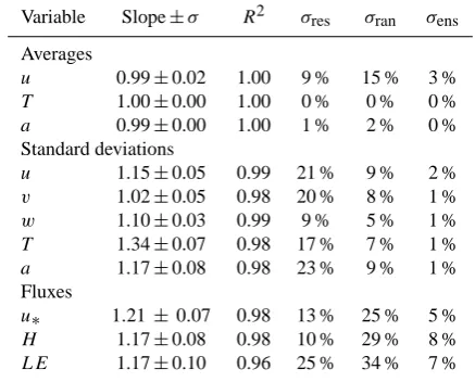
Eqs. (A2)–(A5). In Table 2, the errors are summarized for each variable in the comparison between tower and WSMA. The average random errors are low for the measurement of averages (<1–15 %) and standard deviations (5–9 %), and higher for the friction velocity and the heat fluxes (25–34 %). Likewise, σens increases from averages and SDs to fluxes.
The comparison of the entire dataset between tower and WSMA is associated with an overall uncertainty of≤3 % for the averages,≤2 % for SDs and≤8 % for the fluxes. In the following sections, these errors are used to derive the maximum likelihood functional relationships between tower and WSMA measurements.
3.3.2 Averages
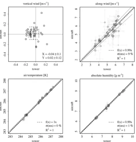
The averages of vertical and along-wind components, tem-perature and absolute humidity were compared between tower and airborne measurements. The vertical wind mea-surements agree within several centimetres and show similar variability (Fig. 2). Taking into account the natural scatter in the data, the average vertical wind is not significantly differ-ent from zero for both platforms. This confirms our assump-tion that the aircraft vertical wind (in geodetic normal) is per-pendicular to the spatial average of the streamlines. For the along-wind component, temperature and humidity measure-ments, the maximum likelihood relationship between tower and WSMA was calculated (Fig. 2). The error bars corre-spond to the random statistical error in the measurements, and the weight of each point in the relationship is represented by the size of the circles. Also shown are the slopef (x),
Table 2. Results of the maximum likelihood functional relation-ships between tower and WSMA measurements. Shown are the MLFR slope and its standard error Slope±σ, weighted coefficient of determinationR2, residual standard errorσres, the average ran-dom statistical errorσranand the ensemble random errorσens.
Variable Slope±σ R2 σres σran σens
Averages
u 0.99±0.02 1.00 9 % 15 % 3 % T 1.00±0.00 1.00 0 % 0 % 0 % a 0.99±0.00 1.00 1 % 2 % 0 % Standard deviations
u 1.15±0.05 0.99 21 % 9 % 2 % v 1.02±0.05 0.98 20 % 8 % 1 % w 1.10±0.03 0.99 9 % 5 % 1 % T 1.34±0.07 0.98 17 % 7 % 1 % a 1.17±0.08 0.98 23 % 9 % 1 % Fluxes
u∗ 1.21 ±0.07 0.98 13 % 25 % 5 %
H 1.17±0.08 0.98 10 % 29 % 8 % LE 1.17±0.10 0.96 25 % 34 % 7 %
the residual standard errorσresand the weighted coefficient
of determinationR2of the MLFR. Along-wind, temperature and humidity measurements agree well between the two plat-forms. The slopes are not significantly different from unity, and the MLFR explains≥99 % of the variance in the dataset. In case of temperature and humidity, the 99.5 % confidence intervals are actually too narrow to be distinguished from the MLFR line. In order to assess the integrity of the MLFR, the results can be compared to the average- and the ensem-ble random errorsσranandσens, respectively. The error in the
residualsσresmeasures the random scatter not accounted for
by the MLFR, and should be lower than the average random errorσran. In the presented data,σresis belowσran(Table 2),
indicating that the significance of the MLFR exceeds the av-erage random error. Likewise, we expect more confidence in the MLFR slope when the ensemble random errorσensis
small. Here the errors in the slopes andσensare equally small,
emphasizing the close relationships. 3.3.3 Spectra and standard deviations
Fig. 1. Smoothed power spectra of acceleration measurements in the WSMA trike coordinate system. The dashed vertical line indicates the −3 dB frequency (20 Hz) of the Butterworth low-pass filter in the wind vector data acquisition system.
Fig. 2. Comparison between tower and WSMA averages of vertical-and along-wind components, temperature vertical-and absolute humidity. Average and standard deviation are given for the vertical wind. For along-wind, temperature and humidity, the solid, dashed and dotted lines are the 1:1 line, the maximum likelihood functional relation-ship, and the 99.5 % confidence interval, respectively. Additional information is given in the text.
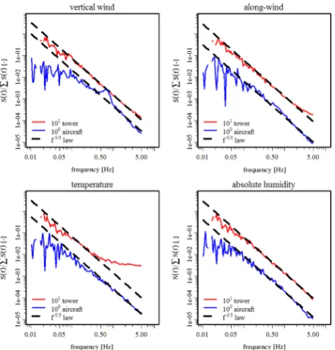
are presented as function of observation frequency to enable the association with the physical properties of the WSMA. Due to fewer samples per dataset, the scatter in the WSMA spectra is higher at low frequencies. We use the streamwise component of the horizontal wind, i.e. in the direction of the mean wind and in the direction of the mean aircraft head-ing for tower and WSMA, respectively. The sonic ture spectrum at the tower is compared to the air tempera-ture spectrum at the WSMA. Kolmogorov (1941) defined the f−5/3 law of isotropic turbulence for the inertial sub-range of atmospheric turbulence (≈0.05–5 Hz). All variables, with exception of the WSMA vertical wind and the tower sonic temperature, follow thef−5/3law well (Fig. 3). The vertical wind and to a lesser degree also the streamwise wind compo-nent of the WSMA show a spectral peak between 0.4–2 Hz, coinciding with the wing’s natural frequency (Sects. 3.2 and 4). Compared to thef−5/3law and relative to the entire fre-quency range, the standard deviations in the wind compo-nents are overestimated by 8±3 % and 2±1 %, respectively (median differences). In the WSMA transverse direction, the wind SD is overestimated by 5±4 % at lower frequencies from 0.15–0.4 Hz (not shown). On the other hand, the power spectrum of the tower sonic temperature does not follow the f−5/3 law very well. For frequencies above 0.3 Hz, the SD is overestimated by 29±19 %. The pattern is consistent for both sonic anemometers at different measurement heights.
Fig. 3. Average power spectra of all measurements between tower and WSMA. To improve legibility, the tower data are offset by one order of magnitude. Also shown is thef−5/3law of isotropic tur-bulence (dashed line). Additional information is given in the text.
(Fig. 4). To a lesser degree, this behaviour is also found in the SD of the cross-wind component (2 %, not shown). Also for temperature (34 %) and humidity (17 %), the WSMA mea-sures higher SDs compared to the tower. However, the dif-ference is significant only for the temperature measurement, while the 99.5 % confidence intervals for all other measure-ments approximately include unity slope. All MLFRs explain ≥98 % of the variance in the data. The ensemble random er-rors are smaller than the slope erer-rors, but the residual stan-dard errors exceed their respective average random statistical error (Table 2). This can partially be attributed to very small denominators in the calculation ofσres, but it is also a
re-sult of the natural scatter in the data. This indicates thatσran
andσensare potentially overoptimistic estimates of the
spa-tial variability in the scalar fields. 3.3.4 Cospectra and fluxes
The correlation of horizontal and vertical wind components was compared between tower (−0.31±0.14) and WSMA (−0.33±0.13) measurements. Both values are close to one another and within the characteristic range from−0.15 to −0.35 (e.g. Foken et al., 2004). However, increased correla-tion due to spectral properties of the WSMA would result in systematically biased EC fluxes. In the following, we quan-tify to what extent the spectral properties of the WSMA con-taminate the measured fluxes, and we correct the resulting bias. For this purpose, cospectra of the fluxes of momentum,
Fig. 4. Comparison between tower and WSMA standard deviations. The results are displayed in the same way as Fig. 2. Additional in-formation is given in the text.
Fig. 5. Average cospectra of all measurements between tower and WSMA. Also shown is the reference cospectrum of Massman and Clement (2004, dashed line). Additional information is given in the text.
the WSMA flux measurement, all individual cospectra are compared between the WSMA and the reference cospectrum in the frequency rangef =0.4–2 Hz of the spectral artifacts. To account for the influence of stratification, the peaks of the reference cospectra were calculated using the forms of Kaimal et al. (1972). Relative to the entire frequency range, the spectral artifacts lead to a systematic deviation in the fluxes of momentum, sensible- and latent heat of 3±6 %, −1±6 % and 1±3 % (median differences), respectively. Sim-ilarly, the inadequate frequency response of the tower sonic temperature measurements results in an underestimation of the sensible heat flux of−3±5 % for frequencies>0.3 Hz. The covariances of the individual measurements were cor-rected for spectral artifacts before continuing the compari-son. Finally, fluxes of momentum, sensible and latent heat are compared between EC measurements from tower and WSMA using the maximum likelihood functional relation-ship (Fig. 6). The WSMA estimates are 17–21 % higher com-pared to the tower, and the 99.5 % confidence intervals en-close unity slope. Alike the SDs, the ensemble random errors of the heat fluxes are less than or equal to the slope errors (Ta-ble 2). This indicates a sufficient sample size supporting the MLFR results. The explained variance is high (≥96 %) for all observed fluxes. All residual standard errors are≤25 %, and significantly lower than the respective average random statistical error (Table 2).
Our analysis revealed that differences in the measurements between tower and weight-shift microlight aircraft partially originate from spectral artifacts. After factoring in these ef-fects, the SDs at the WSMA differ from the tower by 2–15 % for the wind components, 34 % for temperature and 17 % for the humidity measurement. Likewise, the EC fluxes from WSMA remain in excess of 17–21 % compared to the tower.
3.4 Spatial analysis
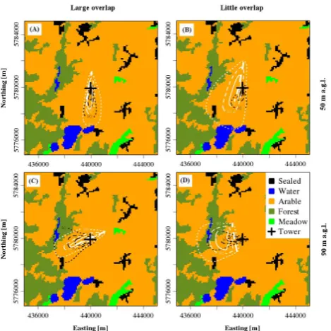
In the following, we investigate whether the remaining dif-ferences between WSMA and tower measurements can be related to their spatial representativeness. For this purpose, we use a cross-wind distributed footprint parameterization (Appendix B) together with the Corine 2006 Land Cover raster. The contributions from all raster cells are cumulated with distance from the measurements, resulting in footprint effect level rings (Fig. 7). When considering the average foot-print contributions over all tower-WSMA comparison mea-surements, the spatial context of the platforms appears to agree quite well. For both platforms, most of the footprint covers arable land (95–97 %). Contributions from the re-maining land covers are sub-percent except for forest (2– 3 %), and meadows do not contribute at all.
Taking a closer look at the individual, simultaneous mea-surements, the source areas can however differ considerably (Fig. 7). The degree of overlap is less related to flight alti-tude than to flight direction. The footprints often agree bet-ter for flights in along-wind direction (Fig. 7a, c). Yet this is not a general rule, because the flight paths are horizontally displaced from the tower (Fig. 7b). For flights in cross-wind direction, the footprint fans out, which additionally reduces the overlap (Fig. 7d). Over all measurements, the overlap ranges from 12–68 % of the footprint weights, with a median of 35±17 %. However, varying overlap did not systemati-cally alter the differences in the flux measurements between tower and WSMA (R2≤0.07).
3.5 Comparison with large-aperture scintillometer
Fig. 6. Comparison between tower and WSMA eddy-covariance fluxes: friction velocity, sensible heat and latent heat. The results are displayed in the same way as Fig. 2. The data points in the shaded areas close to zero are omitted in the calculation of the normalized random errors (see Appendix A). Additional information is given in the text.
Fig. 7. Footprint effect levels of four simultaneous tower and WSMA measurements against the background of the Corine Land Cover raster (10×10 km). The flight path (white dashed line) and the footprint effect levels are shown. Solid, dashed and dotted lines represent a cumulative footprint of 30 %, 60 % and 90 %, respec-tively. Flights (A) and (B) on 15 October 2008, 14:51–14:52 UTC and 14:09–14:12 UTC at 50 m a.g.l. Flights (C) and (D) on 16 Oc-tober 2008, 11:36–11:38 UTC and 11:09–11:10 UTC at 90 m a.g.l.
from the LAS, 55 W m−2and 45 W m−2on 20 and 21
Oc-tober 2008, respectively. Similarly, the measuring heights (Fig. 8, ordinate) are normalized by the boundary layer depth, 450 m and 600 m on 20 and 21 October 2008, respectively. Under conditions of forced convection,Hcan be assumed to diminish below the entrainment zone around 0.8 ABL depth (Deardorff, 1974; Sorbjan, 2006). This allows us to approxi-mate the vertical gradient ofH, for which the measurements
of LAS and 2.4 m EC are used as surface flux reference. The tower measurements at 50 m and 90 m approximately follow the vertical flux gradient derived from the EC surface flux measurements. However, it is evident that anyH measured by tower EC and extrapolated to flight altitude is lower by 25–40 % compared to the LAS. At the same time,H mea-sured by the WSMA is≤25 % lower compared to the LAS, but 15–25 % higher compared to the tower measurements.
Differing source areas of the measurements (Fig. 9) qual-ify as a potential reason for the observed differences in the sensible heat flux. In absence of a better estimate, the LAS footprint was derived from the turbulence statistics at the 50 m tower EC measurement, and weighted along the LAS path (Meijninger et al., 2002; Wang et al., 1978). While southerlies prevailed on 20 October 2008 (Fig. 9a), south-westerly winds were observed on 21 October 2008 (Fig. 9b). Despite weaker winds on 20 October 2008, the footprint extent of the tower measurements is longer compared to 21 October 2008. This can be explained by different sur-face roughness upwind of the measurements and correspond-ing differences in the mechanical generation of turbulence (0.2< u∗<0.5). The roughness lengths are≈10−4m
(wa-ter upwind) and≈10−2m (forest upwind) on 20 and 21 Oc-tober 2008, respectively.
Fig. 8. Vertical profile of the sensible heat flux during two flights: 20 October 2008, 10:53–10:55 UTC (red) and 21 October 2008, 09:56–09:59 UTC (blue). Heat fluxes are compared between large-aperture scintillometer (LAS), tower eddy covariance at 2.4 m, 50 m and 90 m (TOW02, TOW50, TOW90) and the weight-shift micro-light aircraft (WSMA). Where available, error bars show the ran-dom statistical error and the altitude standard deviation. Additional information is given in the text.
4 Discussion
The propagation of sensor errors enables defining the mini-mum change in an atmospheric quantity that can be reliably resolved by the WSMA measurements of respective vari-ables. For the wind measurement, this coincides with the lower margin of the standard deviations observed at both tower and WSMA (Fig. 4). We thus conclude that the pre-cision of the wind measurement warrants eddy-covariance flux measurements under unstable to slightly stable stratifi-cations. The precision of the vertical wind is better by a fac-tor of two compared to the horizontal wind components. This can be traced back to the better precision of the attack- and pitch (≤0.08◦) angles compared to the sideslip- and head-ing (≤0.18◦) angles. From the assessment of sensor accura-cies, we found that the wind and scalar measurements facili-tate the signal levels required for the resolution of mesoscale ABL structures. This enables extending averaging intervals and spectral analyses up to a scale of tens of kilometres.
The focus of this study is on the comparison of turbu-lence statistics between weight-shift microlight aircraft and tower measurements. A potential source of uncertainty is the flow distortion correction of the USA-1 sonic anemome-ters used at the tall tower. Two different corrections are pro-vided by the manufacturer, of which the “milder” 2-D version was used in the operational setup of the DWD. A post pro-cessing comparison for the presented tower data shows that the 3-D version would lead to a systematic increase in the wind SDs by≈35 %, and in the fluxes by≈15 %. From in-strument comparison, the 2-D correction seems to be more
Fig. 9. Footprint effect levels of the measurements from Fig. 8 on 20 October 2008 (A) and 21 October 2008 (B), presented similarly to Fig. 7. In addition, the weighted footprint along the LAS path is shown (red), and the footprints from the tower measurements at 50 m (black) and 90 m (yellow) are distinguished.
appropriate. However, it must be noted that the magnitude of this correction alone is in the order of the differences in the wind SDs and the fluxes observed between the tower and the WSMA. Longer averaging intervals at the tower or detrend-ing of the WSMA data did not change the general behaviour, but increased the scatter in the comparison. Moreover, verti-cal flux divergence can be ruled out as potential error source, since the measurements were conducted at approximately the same altitude above ground. Also, altitude fluctuations by the WSMA were accounted for by using potential quantities of temperature and densities at the tower pressure level. In the following, we consequently focus on the effects of spectral artifacts and surface heterogeneity.
from the comparison of measured spectra and cospectra to modelled ones.
Because of large scatter in the momentum flux cospectra at the tower, no ensemble was calculated. We speculate that the scatter originates from the wind direction-dependent cor-relation of the horizontal and vertical wind components at the USA-1 sonic anemometers (e.g. Mauder et al., 2007b). The erroneous sonic temperature spectrum indicates prob-lems with the measurement of the temperature SD and the sensible heat flux at the tower. The amplitude resolution test by Vickers and Mahrt (1997) would reject 28 out of 36 tower sonic temperature data sets. The problem was related to the insufficient sonic temperature resolution (0.01 K) of the USA-1, which appears as superficial spectral energy in the form of high-frequency white noise. Spectral correction factors analogous to the WSMA measurements were used in an attempt to correct the systematic overestimation of the temperature SD. Such a procedure changes the maximum likelihood functional relationship between tower and aircraft temperature SD from−9 % underestimation to 34 % over-estimation of the WSMA measurement. At the same time, the residual standard error in the MLFR increases from 9 % to 17 %. The scattering can be suppressed by rejecting data points with weak temperature SD (<0.05 K), resulting in a reduced overestimation of 15 % of the WSMA measurement. Consequently, the USA-1 measurements cannot be regarded as reliable reference for the temperature SD, and the spec-tral correction factors must be interpreted with caution. The problem is less pronounced for the sensible heat flux. The white noise in the USA-1 sonic temperature measurement does not affect the measurement of, or the correlation with, the vertical wind measurement. The result is a modest un-derestimation of−3 % of the tower sensible heat flux due to reduced coherence of sonic temperature and vertical wind at high frequencies. The humidity measurements agree well be-tween the platforms in the time and in the frequency domain. Several outliers in the WSMA latent heat flux measurement coincide with WSMA flights west of the tall tower, which are closer to a forest edge. Increased mechanical turbulence downwind of the forest edge is a potential explanation for in-creased turbulent fluxes. This finding however does not hold for the sensible heat flux and the friction velocity, which is in contradiction to scalar similarity.
As a potential source for the observed differences, we as-sess the spatial context of the tower and aircraft measure-ments. The footprint results illustrate that the land cover con-tributions are very similar for both platforms. Provided the land cover data are a suitable proxy for the land-atmosphere exchange, differences between tower and WSMA measure-ments cannot be attributed to different land cover contri-butions alone. However, the footprint analysis also reveals that the source areas only share a fractional overlap. Con-sequently, the observed differences can potentially originate from the platforms’ principally different sampling strategies. Foken (2008) and Mahrt (2010) conclude that the energy
balance non-closure frequently observed from tower EC measurements is connected to the interaction of terrain het-erogeneity and turbulent scales. For this purpose, the trans-fer of heat between surface and atmosphere is considered separately for smaller, random eddies and for larger, non-propagating eddies. Thereof, the transfer by the small, ran-dom eddies is measured by the tower EC. However, an ad-ditional transfer component is suspected to occur at signif-icant surface heterogeneities, leading to the generation of non-uniformly distributed NPEs. Based on intensive mea-surement campaigns and modelling efforts, the presence of NPEs in the study area has been shown (Uhlenbrock et al., 2004). At 100 m measuring height, the resulting average hor-izontal imbalance of the sensible heat flux is in the order of 4–19 % (Steinfeld et al., 2007). In the same study area, Beyrich et al. (2006) found comparable differences between surface flux estimates from aircraft and tower of 11 % for the sensible heat and 23 % for the latent heat. Furthermore, a tendency was shown to close the energy balance on the re-gional scale with spatially averaging methods (Mauder et al., 2007a). This suggests that the tower EC cannot adequately capture all flux contributions due to its inability of spatial sampling. On the other hand, a large-aperture scintillometer captures NPEs up to the dimension of its path length, with increasing sensitivity towards the centre of the path (Foken et al., 2010). Also airborne EC is capable of spatial sampling and captures some of the associated flux, depending on the horizontal extent of the NPEs and the flight path. Therefore, the presence of NPEs in the study area can be considered a potential explanation for the deviation of the tower EC sults from the WSMA, and even more so from the LAS re-sults. In order to further adjust results from tower and air-borne EC measurements, the raw data could be high-pass fil-tered, which restricts low-frequency flux contribution to an identical threshold (e.g. Thomas et al., 2012).
This study combines several principles and methods for the purpose of quantifying: (i) the suitability of airborne in-strumentation for EC measurements, (ii) the complex feed-back of WSMA motions on the EC measurement, and (iii) the direct intercomparison of measurement platforms with differing spatial representativeness. The applied tech-niques are not restricted to use with the WSMA, but are gen-eral enough to be used for the development and assessment of other airborne platforms.
5 Conclusions
on the order of 15–25 % remain between the fluxes measured by the ground-based instruments and the WSMA. At that, the LAS generally measured the highest flux magnitude, fol-lowed by the WSMA and the tower. However, the 99.5 % confidence intervals of the maximum likelihood functional relationships between tower and WSMA include unity slope. Consequently, the observed differences can be considered in-significant, and the accuracy of the WSMA flux measure-ment is quantified to≤10 % (1σ slope error).
Nevertheless, several potential reasons for the disagree-ment of the results between the measuredisagree-ment platforms are investigated. (i) The WSMA wind and flux measurement is subject to spectral artifacts originating from its wing, and the results are corrected prior to the comparison. (ii) The flow distortion correction and the temperature resolution at the tower sonic anemometer measurement alone can explain the full magnitude of the disagreement. (iii) A footprint analysis allows excluding differences in the surface areas as the pri-mary reason for the disagreement. (iv) Principal differences between spatially and temporally averaging flux measure-ments may also explain the observed differences. In partic-ular, energy transfer by non-propagating eddies above het-erogeneous terrain is discussed as a potential reason.
We conclude that the WSMA is a suitable tool to promote the on-going research of surface-atmosphere interactions in heterogeneous landscapes. The flux measurement is suffi-ciently accurate to cover the required flight transect length (10–100 km). Moreover, the WSMA’s low ratio of true air-speed to climb rate is well suited for terrain-following flight over complex terrain. Using e.g. wavelet analysis, the re-gional turbulent exchange measured from the aircraft can be located in space and in spectral scale (Mauder et al., 2007a; Strunin and Hiyama, 2004). All of the above features are ben-eficial for the study of yet poorly understood exchange mech-anisms between the Earth’s surface and the atmosphere. This further substantiates the versatility of the WSMA as a low cost and widely applicable environmental research aircraft.
Appendix A
Integral length scales and statistical error
The integral length scaleλcan be interpreted as the typical size of the most energy-transporting eddies. It is calculated by integration of the autocorrelation function from zero lag to the first crossing with zero at lagr0(Bange et al., 2002;
Lenschow and Stankov, 1986):
λ= r0 Z
0
hf0(x)f0(x+r)i
hf0(x)2i dr . (A1)
Here f represents a turbulent quantity c (scalars or wind components), but also combinations of these with the vertical windf (x)=w0(x)·c0(x)(Bange, 2007). Hence, the integral
scales of the turbulent fluxes were directly calculated from the data of the weight-shift microlight aircraft. The transfor-mation into the integral time scaleτ of simultaneous tower measurements is carried out by division ofλwith the mean horizontal wind speed at the tower. This assumes that Tay-lor’s hypothesis of frozen turbulence is valid (Taylor, 1915). The random statistical error of the sample averagef¯is sim-ply the square root of its variance
q
(f0)2. However, the
er-rors in the varianceV off, or the covarianceF of its combi-nations, are functions of the integral scalesλ,τ. The random statistical errorsσV andσF were determined after Lenschow
and Stankov (1986); Lenschow et al. (1994):
σV2=2·V2· λ
L , (A2)
σF2=2·F2· λ L ·
1+rwc2 r2
wc
, (A3)
with the averaging lengthL and the correlation coefficient between vertical wind and the turbulent quantityrwc. It is
as-sumed thatλL, and thatwandcare Gaussian distributed. The momentum flux consists of two orthogonal components, u0w0 andv0w0, with the wind componentsu,v andw. The
calculation of its random error is obtained from Gaussian er-ror reproduction of the erer-rors in its components (Bange et al., 2002). The individual random errors of the WSMA and the tower measurement,σairandσtow, respectively, were
summa-rized for each variable over all flight legs:
σran= n
P
air
σair+ n
P
tow
σtow
2n−1 , (A4)
resulting in the average random error in the data couplesσran
with the sample sizen. The ensemble random errorσens
con-siders the reduction of the random error with the sample size (Mahrt, 1998):
σens=
σran √
n , (A5)
with zero expected valueσensand the standard deviationσran
of the population. While σran is a measure for the average
dispersion of the data couples, σens quantifies the level of
confidence we can expect from comparing the entire dataset between the two platforms. To use Eqs. (A4)–(A5) for data obtained during different flight days, we use normalized er-ror estimates. Yet, the normalized erer-rors are excessively large when the denominator, i.e. the measurement quantity, ap-proaches zero. For turbulent fluxes, this is usually the case under stable conditions, where e.g. intermittent turbulence can violate the assumptions in the integral length scales. Con-sequently, we constrain the calculation ofσranandσensfor the
fluxes to values of u∗>0.2 m s−1 andH,E >20 W m−2,
Fig. B1. Cross-wind and along-wind integrated distributions of the footprints for case 2,z=100 m from Markkanen et al. (2009). Up-per and lower panels display longitudinal and cross-sections, re-spectively. The footprint weight distributions are shown on the left side, and the cumulative distributions are shown on the right side.
Appendix B
Footprint modelling
The footprint- or source weight function quantifies the spatial contributions to each measurement (Schmid, 2002; Vesala et al., 2008). Analytical footprint models are often limited, e.g. regarding stability regimes or measurement heights (e.g. Kormann and Meixner, 2001, subsequently referred to with KM01). Lagrangian footprint models overcome these lim-itations and additionally consider 3-D dispersion, but are computationally expensive. The footprint model of Kljun et al. (2004, KL04) is a parameterization of the backward Lagrangian model of Kljun et al. (2002, KL02) in the range −200≤z/L≤1,u∗≥0.2 m s−1, and 1 m≤z≤zi, with the
boundary layer depth zi. Thus, it combines little
computa-tional effort with broad applicability. The parameterization depends upon friction velocity u∗, measurement height z,
standard deviation of the vertical windσw and the
aerody-namic roughness lengthz0, of whichu∗,zandσw are
mea-sured directly. The roughness length is inferred using the log-arithmic wind profile with the integrated universal function for momentum exchange after Businger et al. (1971) in the form of H¨ogstr¨om (1988). The KL04 is a cross-wind inte-grated footprint model, i.e. it does not resolve the distribution perpendicular to the main wind direction. In order to account for cross-wind dispersion, the KL04 was combined with
Table B1. Median performance of the footprint parameterizations KL04+ and KM01 compared to the reference Lagrangian model of Kljun et al. (2002). Uncertainty measures NMSE, MAD andrare explained in the text.
Direction Along-wind Cross-wind
Model KL04+ KM01 KL04+ KM01
NMSE 0.34±0.05 0.95±0.48 0.34±0.05 0.33±0.36 MAD [%] 0.43±0.10 0.63±0.28 0.08±0.05 0.12±0.14 r 0.91±0.00 0.66±0.12 0.99±0.01 0.99±0.01
a Gaussian cross-wind distribution function (Kljun et al., 2012). The combination of KL04 with this cross-wind distri-bution results in a computationally fast footprint parameteri-zation which considers 3-D dispersion and is not constrained to applications in the surface layer. In the following, we refer to this model as KL04+.
To evaluate model performance, KM01 and KL04+ were compared to the reference Lagrangian model KL02. For this purpose, four existing realizations of the KL02 model were used from Markkanen et al. (2009, Table 1, case 1 (L= −32 m, u∗=0.27 m s−1) and case 2 (L= −76.6 m, u∗=
0.295 m s−1),z=50 m and 100 m). Markkanen et al. (2009) adopted case 1 from Leclerc et al. (1997), and referenced the results to large eddy simulations (Raasch and Schr¨oter, 2001). The above parameter sets do not includeσvandσw,
which were derived using the integral turbulence characteris-tics proposed by Lumley and Panofsky (1964) and Panofsky et al. (1977), respectively. The computed footprint weights were summarized for each cell of a grid with 100 m hori-zontal spacing and subsequently integrated over cross-wind and along-wind direction, respectively (Fig. B1). In both directions, KL04+ assigns more weight to the close range compared to KM01 (Fig. B1 left panels). This is consis-tent throughout the range of the tested atmospheric condi-tions (not shown). In along-wind direction, KL04+ repro-duces KL02 very well until the cumulative distribution ac-counts for approximately 80 % of the footprint (Fig. B1 upper right panel). Contributions from below the measurement lo-cation due to along-wind dispersion are slightly pronounced by KL04+, and neglected by KM01. The cross-wind distribu-tions of both KL04+ and KM01 agree reasonably well with KL02.
comparison. In both along-wind and cross-wind directions, the similarity between KL04+ and KL02 is as good or bet-ter than between KM01 and KL02 (r). In along-wind di-rection, KL04+ is considerably closer to KL02 in the close range (NMSE) and the far range (MAD) compared to KM01. A similar deviation between KM01 and KL02 has been re-ported by Kljun et al. (2003). In cross-wind direction, both KL04+ and KM01 agree equally well with KL02. For all metrics, the standard errors over the four parameter sets are smaller for the KL04+ model, pointing out its reliability.
Acknowledgements. Recognition has to be given to Frank Neidl
and Rainer Steinbrecher at the Karlsruhe Institute of Technol-ogy, Institute for Meteorology and Climate Research. Neidl programmed and continuously maintained the data acquisition system, while Steinbrecher initiated wind- and flux measurements with the weight-shift microlight aircraft in the first place. Thanks go to Ulrich Weisensee and Jens-Peter Leps at the German Meteorological Service, Richard-Aßmann-Observatory Lindenberg for performing the tower turbulence measurements. We are obliged to Xunhua Zheng and her workgroup at the Chinese Academy of Sciences, Institute of Atmospheric Physics, which was hosting our project and providing indispensable infrastructure. Our thanks to Jens Bange at the Eberhard Karls University of T¨ubingen, Institute for Geoscience, for his advice regarding the flight campaign design. The authors wish to thank Henry Loescher at the National Ecological Observatory Network, Fundamental Instrument Unit for his continued support. Stipend funding by the German Academic Exchange Service, Helmholtz Association of German Research Centres, China Scholarship Council and the European Union under the Science and Technology Fellowship China is acknowledged. The National Ecological Observatory Network is a project spon-sored by the National Science Foundation and managed under cooperative agreement by NEON, Inc. This material is based upon work supported by the National Science Foundation under the grant DBI-0752017. Any opinions, findings, and conclusions or recommendations expressed in this material are those of the authors and do not necessarily reflect the views of the National Science Foundation.
Edited by: S. Malinowski
References
Bange, J.: Airborne Measurement of Turbulent Energy Exchange Between the Earth Surface and the Atmosphere, Faculty of Engineering, Braunschweig University of Technology, Braun-schweig, Germany, 2007.
Bange, J., Beyrich, F., and Engelbart, D. A. M.: Airborne mea-surements of turbulent fluxes during LITFASS-98: Compari-son with ground measurements and remote sensing in a case study, Theor. Appl. Climatol., 73, 35–51, doi:10.1007/s00704-002-0692-6, 2002.
Betts, A. K., Desjardins, R. L., Macpherson, J. I., and Kelly, R. D.: Boundary-layer heat and moisture budgets from FIFE, Bound.-Lay. Meteorol., 50, 109–138, doi:10.1007/BF00120520, 1990.
Beyrich, F. and Adam, W. K.: Site and data report for the Linden-berg reference site in CEOP – phase I, Berichte des Deutschen Wetterdienstes, 55 pp., 2007.
Beyrich, F., Leps, J. P., Mauder, M., Bange, J., Foken, T., Huneke, S., Lohse, H., Ludi, A., Meijninger, W. M. L., Mironov, D., Weisensee, U., and Zittel, P.: Area-averaged surface fluxes over the LITFASS region based on eddy-covariance measurements, Bound.-Lay. Meteorol., 121, 33–65, doi:10.1007/s10546-006-9052-x, 2006.
Businger, J. A., Wyngaard, J. C., Izumi, Y., and Bradley, E. F.: Flux-profile relationships in the atmospheric surface layer, J. Atmos. Sci., 28, 181–189, doi:10.1175/1520-0469(1971)028<0181:FPRITA>2.0.CO;2, 1971.
Chen, J., Jonsson, P., Tamura, M., Gu, Z. H., Matsushita, B., and Eklundh, L.: A simple method for reconstructing a high-quality NDVI time-series data set based on the Savitzky-Golay filter, Remote Sens. Environ., 91, 332–344, doi:10.1016/j.rse.2004.03.014, 2004.
Davis, F. W., Schimel, D. S., Friedl, M. A., Michaelsen, J. C., Kittel, T. G. F., Dubayah, R., and Dozier, J.: Covariance of biophysical data with digital topographic and land use maps over the FIFE site, J. Geophys. Res.-Atmos., 97, 19009–19021, doi:10.1029/92jd01345, 1992.
Deardorff, J. W.: Three-dimensional numerical study of turbulence in an entraining mixed layer, Bound.-Lay. Meteorol., 7, 199–226, doi:10.1007/bf00227913, 1974.
Desjardins, R. L., MacPherson, J. I., Schuepp, P. H., and Karanja, F.: An evaluation of aircraft flux measurements of CO2, water vapor and sensible heat, Bound.-Lay. Meteorol., 47, 55–69, doi:10.1007/BF00122322, 1989.
Desjardins, R. L., MacPherson, J. I., Mahrt, L., Schuepp, P., Pat-tey, E., Neumann, H., Baldocchi, D., Wofsy, S., Fitzjarrald, D., McCaughey, H., and Joiner, D. W.: Scaling up flux measurements for the boreal forest using aircraft-tower combinations, J. Geo-phys. Res.-Atmos., 102, 29125–29133, doi:10.1029/97JD00278, 1997.
Egger, J., Bajrachaya, S., Heinrich, R., Kolb, P., Lammlein, S., Mech, M., Reuder, J., Schaper, W., Shakya, P., Schween, J., and Wendt, H.: Diurnal winds in the Himalayan Kali Gan-daki valley. Part III: Remotely piloted aircraft soundings, Month. Weather Rev., 130, 2042–2058, doi:10.1175/1520-0493(2002)130<2042:DWITHK>2.0.CO;2, 2002.
Foken, T.: The energy balance closure problem: an overview, Ecol. Appl., 18, 1351–1367, doi:10.1890/06-0922.1, 2008.
Foken, T., G¨ockede, M., Mauder, M., Mahrt, L., Amiro, B., and Munger, W.: Post-field Data Quality Conirol, in: Handbook of Micrometeorology: A Guide for Surface Flux Measurement and Analysis, 1st Edn., edited by: Lee, X., Law, B., and Mass-man, W., Springer Netherlands, Dordrecht, The Netherlands, 264 pp., 2004.
Foken, T., Mauder, M., Liebethal, C., Wimmer, F., Beyrich, F., Leps, J.-P., Raasch, S., DeBruin, H. A. R., Meijninger, W. M. L., and Bange, J.: Energy balance closure for the LITFASS-2003 experiment, Theor. Appl. Climatol., 101, 149–160, doi:10.1007/s00704-009-0216-8, 2010.
Heidel-berg, London, New York, 85–131, 2012.
Garman, K. E., Hill, K. A., Wyss, P., Carlsen, M., Zimmerman, J. R., Stirm, B. H., Carney, T. Q., Santini, R., and Shepson, P. B.: An airborne and wind tunnel evaluation of a wind turbulence mea-surement system for aircraft-based flux meamea-surements, J. Atmos. Ocean. Tech., 23, 1696–1708, doi:10.1175/JTECH1940.1, 2006. G¨ockede, M., Foken, T., Aubinet, M., Aurela, M., Banza, J., Bern-hofer, C., Bonnefond, J. M., Brunet, Y., Carrara, A., Clement, R., Dellwik, E., Elbers, J., Eugster, W., Fuhrer, J., Granier, A., Gr¨unwald, T., Heinesch, B., Janssens, I. A., Knohl, A., Koeble, R., Laurila, T., Longdoz, B., Manca, G., Marek, M., Markka-nen, T., Mateus, J., Matteucci, G., Mauder, M., Migliavacca, M., Minerbi, S., Moncrieff, J., Montagnani, L., Moors, E., Ourcival, J.-M., Papale, D., Pereira, J., Pilegaard, K., Pita, G., Rambal, S., Rebmann, C., Rodrigues, A., Rotenberg, E., Sanz, M. J., Sed-lak, P., Seufert, G., Siebicke, L., Soussana, J. F., Valentini, R., Vesala, T., Verbeeck, H., and Yakir, D.: Quality control of Car-boEurope flux data – Part 1: Coupling footprint analyses with flux data quality assessment to evaluate sites in forest ecosys-tems, Biogeosciences, 5, 433–450, doi:10.5194/bg-5-433-2008, 2008.
Hanna, S. R. and Paine, R. J.: Hybrid Plume Disper-sion Model (HPDM) development and evaluation, J. Appl. Meteorol., 28, 206–224, doi:10.1175/1520-0450(1989)028<0206:HPDMDA>2.0.CO;2, 1989.
Hiyama, T., Strunin, M. A., Tanaka, H., and Ohta, T.: The devel-opment of local circulations around the Lena River and their ef-fect on tower-observed energy imbalance, Hydrol. Process., 21, 2038–2048, doi:10.1002/hyp.6705, 2007.
Hobbs, S., Dyer, D., Courault, D., Olioso, A., Lagouarde, J. P., Kerr, Y., McAneney, J., and Bonnefond, J.: Surface layer pro-files of air temperature and humidity measured from unmanned aircraft, Agronomie, 22, 635–640, doi:10.1051/agro:2002050, 2002.
H¨ogstr¨om, U.: Non-dimensional wind and temperature profiles in the atmospheric surface layer: A re-evaluation, Bound.-Lay. Me-teorol., 42, 55–78, doi:10.1007/BF00119875, 1988.
Hojstrup, J.: A statistical data screening procedure, Meas. Sci. Tech-nol., 4, 153–157, doi:10.1088/0957-0233/4/2/003, 1993. Isaac, P. R., Leuning, R., Hacker, J. M., Cleugh, H. A.,
Cop-pin, P. A., Denmead, O. T., and Raupach, M. R.: Estima-tion of regional evapotranspiraEstima-tion by combining aircraft and ground-based measurements, Bound.-Lay. Meteorol., 110, 69– 98, doi:10.1023/A:1026054317990, 2004a.
Isaac, P. R., McAneney, J., Leuning, R., and Hacker, J. M.: Comparison of aircraft and ground-based flux measure-ments during OASIS95, Bound.-Lay. Meteorol., 110, 39–67, doi:10.1023/A:1026002301152, 2004b.
Junkermann, W.: An ultralight aircraft as platform for research in the lower troposphere: System performance and first results from radiation transfer studies in stratiform aerosol layers and broken cloud conditions, J. Atmos. Ocean. Tech., 18, 934–946, doi:10.1175/1520-0426(2001)018<0934:AUAAPF>2.0.CO;2, 2001.
Junkermann, W.: The actinic UV-radiation budget during the ES-COMPTE campaign 2001: results of airborne measurements with the microlight research aircraft D-MIFU, Atmos. Res., 74, 461–475, doi:10.1016/j.atmosres.2004.06.009, 2005.
Kaimal, J. C. and Finnigan, J. J.: Atmospheric Boundary Layer Flows: Their Structure and Measurement, Oxford University Press, 289 pp., New York, USA, 1994.
Kaimal, J. C., Wyngaard, J. C., Izumi, Y., and Cot´e, O. R.: Spectral characteristics of surface-layer turbulence, Q. J. Roy. Meteorol. Soc., 98, 563–589, doi:10.1002/qj.49709841707, 1972. Kanda, M., Inagaki, A., Letzel, M. O., Raasch, S., and
Watan-abe, T.: LES study of the energy imbalance problem with Eddy covariance fluxes, Bound.-Lay. Meteorol., 110, 381–404, doi:10.1023/B:BOUN.0000007225.45548.7a, 2004.
Kljun, N., Rotach, M. W., and Schmid, H. P.: A three-dimensional backward lagrangian footprint model for a wide range of boundary-layer stratifications, Bound.-Lay. Meteorol., 103, 205– 226, doi:10.1023/A:1014556300021, 2002.
Kljun, N., Kormann, R., Rotach, M. W., and Meixer, F. X.: Compar-ison of the Langrangian footprint model LPDM-B with an ana-lytical footprint model, Bound.-Lay. Meteorol., 106, 349–355, doi:10.1023/A:1021141223386, 2003.
Kljun, N., Calanca, P., Rotach, M. W., and Schmid, H. P.: A simple parameterisation for flux footprint pre-dictions, Bound.-Lay. Meteorol., 112, 503–523, doi:10.1023/B:BOUN.0000030653.71031.96, 2004.
Kljun, N., Rotach, M. W., and Schmid, H. P.: A Simple Parame-terisation for Two-dimensional Flux Footprints, in preparation, 2012.
Kolmogorov, A. N.: Lokalnaja struktura turbulentnosti v neschtschimaemoi schidkosti pri otschen bolschich tschislach Reynoldsa (The local structure of turbulence in incompressible viscous fluid for very large Reynolds numbers), Proceedings of the USSR Academy of Sciences, 30, 299–303, 1941.
Kormann, R. and Meixner, F. X.: An analytical footprint model for non-neutral stratification, Bound.-Lay. Meteorol., 99, 207–224, doi:10.1023/A:1018991015119, 2001.
Kvalseth, T. O.: Cautionary note aboutR2, Am. Stat., 39, 279–285, 1985.
Leclerc, M. Y., Shen, S., and Lamb, B.: Observations and large-eddy simulation modeling of footprints in the lower convec-tive boundary layer, J. Geophys. Res.-Atmos., 102, 9323–9334, doi:10.1029/96JD03984, 1997.
Lenschow, D. H. and Stankov, B. B.: Length Scales in the Convective Boundary Layer, J. Atmos. Sci., 43, 1198–1209, doi:10.1175/1520-0469(1986)043<1198:LSITCB>2.0.CO;2, 1986.
Lenschow, D. and Sun, J.: The spectral composition of fluxes and variances over land and sea out to the mesoscale, Bound.-Lay. Meteorol., 125, 63–84, doi:10.1007/s10546-007-9191-8, 2007. Lenschow, D. H., Mann, J., and Kristensen, L.: How long is
long enough when measuring fluxes and other turbulence statis-tics?, J. Atmos. Ocean. Tech., 11, 661–673, doi:10.1175/1520-0426(1994)011<0661:HLILEW>2.0.CO;2, 1994.
Lindley, D. V.: Regression lines and the linear functional relation-ship, Supplement, J. R. Stat. Soc., 9, 218–244, 1947.
Liu, H. P., Peters, G., and Foken, T.: New equations for sonic tem-perature variance and buoyancy heat flux with an omnidirec-tional sonic anemometer, Bound.-Lay. Meteorol., 100, 459–468, doi:10.1023/A:1019207031397, 2001.