Multi-objective facility layout problems using BBO, NSBBO and NSGA-II metaheuristic algorithms Pages 239-262 Download PDF

(1)

* Corresponding author

E-mail: [email protected] (D. Singh) 2019 Growing Science Ltd.

doi: 10.5267/j.ijiec.2018.6.006

International Journal of Industrial Engineering Computations 10 (2019) 239–262

Contents lists available at GrowingScience

International Journal of Industrial Engineering Computations

homepage: www.GrowingScience.com/ijiec

Multi-objective facility layout problems using BBO, NSBBO and NSGA-II metaheuristic algorithms

Dinesh Singha*_{and Supriya Ingole}a

a_{S.V. National Institute of Technology, Surat, India} C H R O N I C L E A B S T R A C T

Article history: Received Januar 18 2018 Received in Revised Format May 12 2018

Accepted June 16 2018 Available online June 16 2018

Quantitative and qualitative objectives are both significant to solve any facility layout problem (FLP), which is called as multi-objective FLP. Generally, quantitative factors are considered as material handling cost, time, etc., and qualitative factors are considered as closeness rating, hazardous movement between the facilities, etc. For solving and optimizing two or more objectives, two methods are available. First is weight approach method and second is non-dominated sorting method. In the former method, suitable weights are given to each objective and combined in a single objective function; while in later method, the objectives are defined separately and by making comparison of the solutions on the non-dominance criteria, best Pareto-optimal solutions are obtained. In this paper, equal area multi-objective FLPs which are formulated as quadratic assignment problem (QAP) are considered and optimized using biogeography based optimization (BBO) algorithm and non-dominated sorting BBO (NSBBO) algorithm. BBO is one of the efficient metaheuristic techniques, developed to solve complex optimization problems. Computational results of BBO algorithm using weight approach illustrate its better performance compared to other methods while solving multi-objective FLPs. Furthermore to obtain Pareto optimal solutions, NSBBO algorithm is implemented.

Multi-objective facility layout problems

Weight approach Pareto optimality approach Biogeography-based optimization Non-dominated sorting biogeography-based optimization

1. Introduction

(2)

facilities in the layout are of equal area and identical shape and formulated as QAP. Each facility is assigned to a square block in the layout. The problems are solved using multi-objective optimization.

Singh and Singh (2010)proposed an approach to solve multi-objective FLPs by using weight method. In

this work, the same problems are solved and optimized using BBO algorithm with weight approach and non-dominated sorting biogeography-based optimization (NSBBO) algorithm with Pareto approach. In this paper, BBO and NSBBO algorithms are proposed because it is observed that BBO and NSBBO algorithms are applicable in wide variety of complex optimization problems. BBO and NSBBO are innovative non-traditional optimization techniques and till date, they are not applied to solve multi-objective FLPs. The results obtained using BBO are better than previous employed techniques. The performance of NSBBO is compared with non-dominated sorting genetic algorithm (NSGA-II). The paper further consists of Section 2: Literature review; Section 3: QAP function for multi-objective FLP; Section 4: BBO and NSBBO algorithm; Section 5: Performance evaluation of BBO and NSBBO algorithms for multi-objective FLPs and Section 6: Conclusion.

2. Literature Review

The facility layout of equal and unequal area with single objective function is discussed and solved by

many researchers; however for obtaining more improved results, layout planner should consider more

than one objective while solving FLP. The present literature review focussed on multi-objective FLPs and various heuristic and meta-heuristic techniques used to optimize them. The literature review categorised as follows:

2.1 Multi-objective FLPs using weight approach

Weight method is implemented by many researchers while solving multi-objective FLPs to normalise the different objective functions and obtain the optimal solution. Rosenblatt (1979) first attempted the concept of multi-goal approach for FLPs. Dutta and Sahu (1982) implemented a pairwise exchange heuristic to solve multi-objective FLP considering material handling cost and closeness rating. Fortenberry and Cox (1985) considered material flow as quantitative objective to minimize and closeness rating as qualitative objective to maximize. The objectives are combined using weight approach. Khare et al. (1988) proposed a combined computer-aided approach for multi-objective FLP. They obtained the solutions by summation of objective values at different weightage. Harmonosky and Tothero (1992) formulated a methodology to solve multi-factor FLP by combining the quantitative and qualitative factors

with suitable weights. Chen and Sha (2001) proposed a new approach by considering suboptimal

solutions for large size multi-objective layout problems. Chen and Sha (2005) considered four objectives to solve equal area FLP (namely material handling cost, adjacency requirement, material handling time and hazardous movement between the facilities).

While designing a facility layout, the effect of workflow interference is studied (Chiang et al., 2006) with linear and non-linear formulations of the problem. Ye and Zhou (2007) developed a hybrid algorithm using genetic algorithm (GA) and tabu search to solve multi-objective FLPs having material handling cost and adjacency requirement. They considered unequal area facilities with fixed aisle structure. A multi-goal layout approach is presented by Peer and Sharma (2008) and the objective function consists of closeness relationship and workflow. Material flow factor cost (MFFC), shape ratio factor (SRF) and

area utilisation factor (AUF) are considered by Ku et al. (2011) to determine total layout cost by

conducting a weighted summation of MFFC, SRF and AUF and optimized using parallel GA. Total MHC (quantitative) and the total closeness rating (qualitative) are considered to solve FLP by using weight

assignment method for each objective by Sahin (2011). Matai (2015) proposed modified simulated

annealing (SA) algorithm to solve multi-objective FLP using the weight assignment method introduced

by Singh and Singh (2010). This method is independent of decision maker and thus makes the layout

(3)

D. Singh and S. Ingole / International Journal of Industrial Engineering Computations 10 (2019)

2.2 Multi-objective FLPs using Pareto-optimal approach

This section gives the idea about the Pareto-optimal criteria used to solve multi-objective FLPs in previous literature. Aiello et al. (2006) applied a multi-objective constrained GA to find Pareto-optimal solutions of unequal area FLP and the optimal solution is selected using multi-criteria decision-making

procedure i.e. Electre.They considered four objectives namely, MHC, aspect ratio, closeness request and

distance request between the departments. A dynamic FLP with unequal shape facilities and

pickup-drop-off points explained by Jolai et al. (2012)using multi-objective particle swarm optimization (PSO).

The objectives considered are adjacency, distance request, orientation and rearrangement cost of moving or reorienting departments. A multi objective GA is proposed for solving unequal area FLP with more than one objective function and obtained Pareto-optimal solutions (Aiello et al. 2012).

Hathhorn et al. (2013)considered two objective functions of minimising material handling and facility

building costs and formulated using mixed integer programming (MIP); further they proposed a lexicographic ordering technique to handle multiple objectives. A multi-objective FLP having unequal area facilities with slicing tree representation is approached in two steps by Aiello et al (2013). The first step is to determine Pareto-optimal solutions by using multi-objective GA and the second step is to select the optimal solution by means of the multi-criteria decision-making procedure. A modified SA based approach is presented for solving equal area multi-objective FLP by Matai et al. (2013). An evolutionary

approach is investigated by Ripon et al. (2013) for solving unequal area multi-objective FLP using

variable neighbourhood search (VNS) with an adaptive scheme that presents the final layouts as a set of Pareto-optimal solutions. A mathematical model presented for equal area FLP considering two objectives (i.e. MHC and adjacency requirement) and optimized using a new developed heuristic technique (Chen & Lo, 2014).

2.3 Application of BBO and NSBBO from literature

The literature survey states that a number of meta-heuristic techniques such as GA, PSO, SA, etc., have been implemented to solve multi-objective FLPs, but till now, BBO algorithm is not attempted to solve the FLPs. However, an application of BBO algorithm for machine layout design problems to minimize

the material handling distance is described by Sooncharoen et al. (2015).A hybrid technique is proposed

combining BBO and TS algorithms to solve QAP and obtained better results within reasonable computational time by Lim et al. (2016). Regarding multi-objective BBO, some of its applications are

depicted here. Ma et al. (2012)introduced biogeography-based multi-objective optimization (BBMO) to

solve several test functions and compared with NSGA-II developed by Deb et al. (2002). Further, Simon

(2013)explained objective BBO and NSBBO algorithms to find Pareto optimal solutions of

multi-objective problems. Chutima and Naruemitwong (2014) implemented Pareto-BBO algorithm to solve

mixed-model sequencing problems on a two-sided assembly line by considering three conflicting

objectives. Ma et al. (2015)proposed an ensemble multi-objective BBO (EMBBO) algorithm to solve

the automated warehouse scheduling problem. The EMBBO algorithm constitutes vector evaluated BBO (VEBBO), NSBBO and niched Pareto BBO (NPBBO). A community detection problem in dynamic networks with two objectives is solved using multi-objective BBO algorithm with decomposition mechanism (Zhou et al., 2015).

BBO is a nature-inspired optimization technique which is developed by Simonin 2008 and is based on

the migration characteristic of species from one island to another. Simon (2008) successfully optimized

all the continuous functions by using BBO algorithm. Therefore, by observing the efficiency of BBO and

(4)

Therefore, NSBBO algorithm is implemented to solve multi-objective FLPs to obtain non-dominated solutions and to test the performance of NSBBO algorithm.

3. QAP function for multi-objective FLP

In this paper, two objective functions (i.e. MHC and closeness rating) are considered. The multi-objective

FLP is formulated as QAP (Singh & Singh, 2010).

(1)

(2)

To compare the results with previous methods, weight approach is considered. The objective functions are converted into single-objective function using suitable weights given as below:

(3)

where

f1 -Objective function to minimise the material work flow or MHC

f2 - Objective function to maximise the closeness rating (CR)

n - Number of facility

fij -Work flow from facility i to j

dij - Distance from facility i to j

cij - Closeness rating between facility i and facility j

w - Objective weight for each objective

F1 - Combined objective function

It is observed that Singh and Singh (2010) and Matai (2015) considered the sum of closeness rating as a second objective which is constant for every solution and it is not having contribution towards the improvement of the layout. However, as mentioned by Urban (1987) and Khare et al. (1988), closeness rating is multiplied with the distance between the departments which will provide the actual combined solution of multi-objective FLP. Therefore, second objective is considered as given in Eq. (4) and the combined objective function is shown in Eq. (5).

(4)

(5)

The multi-objective FLPs from (Singh & Singh, 2010)are solved using the objective function considered

by them for making comparison. The same problems are solved using the function in Eq. (5) to observe the difference between the results. Using weighted sum method, each objective function should be given proper weight to obtain the best solution. All factors are normalized before solving the final objective function, as the value of each factor is different from other. For instance, the values of material flow can vary from zero to very large amount while the value of closeness rating can be in the range of 0 to 5.

Singh and Singh (2010)described a capable method to calculate the weights of each objective. For detail

procedure, please refer (Singh & Singh, 2010).To calculate weights for each objective following steps

(5)

Stage1: Matrix normalization

Normalize the matrices of material work flow and closeness rating. The first step is summation of all the elements of each matrix and the second step is dividing each element of the matrix with the sum of all the elements of the matrix.

Stage 2: Objective weight calculation

In this stage, suitable weight of each objective is calculated using four methods proposed by (Singh &

Singh, 2010). These methods are mean weight method (MWM), geometric mean weight method

(GMWM), standard deviation weight method (SDWM) and critical importance through inter criteria correlation method (CRITICM). The weights considered in this paper for solving multi-objective FLPs are directly considered from weights calculated by Singh and Singh (2010).

Stage 3: Solve multi-objective FLP considering above weights using BBO algorithm

Each problem is solved considering the weight values of all the above mentioned methods and optimized using BBO algorithm. Amongst all the methods, whichever is providing minimum objective function value will be considered as best method.

4. Biogeography-based optimization (BBO)

In this section, the working of BBO and NSBBO algorithms are described in details. BBO algorithm is implemented using weight approach to compare with previous results and NSBBO is implemented to obtain Pareto-optimal solutions.

4.1 Introduction to BBO algorithm

BBO is an evolutionary, population-based algorithm (Simon, 2008). This algorithm is based on the

principle of island biogeography in which geographical distribution of biological species is explained (Alroomi et al., 2013). BBO algorithm follows migration and mutation operations to reach global

minimum solution.The mathematical formulation of BBO algorithm is developed by considering the

migration behaviour of species from one place to another. On an island or habitat, if the living conditions are appropriate for species then that habitat have high suitability index (HSI), because this habitat have better features than other habitats. The variables that characterize habitability of an island are called as

suitability index variables (SIVs) (Simon, 2008). Habitats having high HSI consist of more number of

species than that of low HSI habitats. Therefore, the species on the high HSI habitats can emigrate to other habitat and have low species immigration rate as they are already full with species. Similarly, the low HSI habitats have high immigration rate of species because of their low population.

4.1.1 BBO Algorithm

BBO algorithm is established on the concept of distribution of species on islands which converts into a general problem function solution. Each island is considered as one member or solution. By considering

the emigration (μ) and immigration (λ) rates of each member, the information between the habitats is

shared probabilistically.High-HSI habitat represents a good solution and low-HSI habitat represents poor

solution. The good solution means the island has lots of good features such as trees, food, rainfall, temperature, humidity, etc.; therefore this island or habitat has high HSI. Each feature is indicated as SIV, which denotes the independent variable of the problem function or facilities in case of FLP. Good

solution features emigrate from high-HSI islands to low-HSI islands (Rahmati & Zandieh, 2012).A poor

(6)

population in each iteration. If the algorithm traps in local minima, then the elitist solutions will remain intact and gives near-optimal solutions.

4.1.2 Algorithm Steps of BBO

Step 1. Initialisation of BBO parameters

k - Number of islands or number of layouts, each island represents the permutation of

facilities from n =1,2,…..,k

G - Generations of algorithm

I – maximum immigration rate (Fig. 2)

E – maximum emigration rate (Fig. 2)

Smax – Maximum number of species on an island

Step 2. Defining the objective function and finding the objective function value (OFV) of each island or layout

Step 2. Migration of species from one island to another with a probability

Step 3. Mutation is performed to update the islands

Step 4. Calculation of OFV of updated islands

Step 5. Repeat steps 2-4 until best value is obtained or maximum iterations are reached.

4.2 Non-dominated sorting biogeography-based optimization (NSBBO)

NSBBO algorithm is described by Simon (2013).The working of NSBBO algorithm is the same as that

of NSGA-II. To overcome the problem of assigning the proper weights to the objective, NSGA-II is

developed by Deb et al. (2002)for multi-objective optimization problems of continuous functions. The

working of NSGA-II is based on the sorting of non-dominated or Pareto-optimum solutions, calculation of crowding distance and sharing fitness between the solutions. A Pareto frontier is generated when a set of optimal solutions are connected together.

Pareto optimal solutions are called as non-dominated solutions. For understanding, two objective

functions Fi and Fj are considered with two solutions, P1 and P2. If P1 dominates P2 in terms of both

objectives, P1 is dominant over P2. If P1 is not dominated by the other solution, P1 is called the

dominant solution. The set of dominant solutions is called the Pareto front or frontier. A

non-dominated solution can be considered as explained here. Suppose, x∗_{represents a feasible solution while}

x represents some other feasible solution. For a minimization problem, if x∗_{satisfy following two}

conditions

(1) Fi (x*) < Fi (x) and (2) Fj (x*) ≤ Fj (x)( j≠i),

Then x∗ _{is called the non-dominated solution. Therefore, when}_x_∗ _{is a non-dominated solution, its}

objective function value can be equal to or less than other feasible solutions (Chen & Lo, 2014). The non-dominated sorting procedure of NSGA-II is implemented in NSBBO. The crossover and mutation operators of NSGA-II are replaced by migration and mutation operators of BBO algorithm.

4.2.1 NSBBO procedure steps

1. Initialisation

Initial solutions of arbitrary islands are generated. Each island solution is compared with other solutions to find the non-dominant solutions. These island solutions are sorted using non-dominance approach and numbers of Pareto-fronts of final objective values are obtained as discussed in section 4.2. According to non-domination level, each solution is allotted a fitness or rank. The first front of subpopulation of islands

(7)

2. Crowding distance calculation

After obtaining non-dominated solutions, crowding distance is calculated; this is the distance between the islands. The distance is calculated to get an evaluation of the concentration of solutions nearby a particular point in the population of islands. The crowding distance provides an estimate of the density

of solutions around each solution belonging to the same front. Suppose, n number of solutions belonging

to the same feasible front, so these solutions are sorted in descending order, with respect to an objective

K. The crowding distance is shown in Fig. 1.

(6)

(i = 2, 3, . . ., n-1) and (K= 1, 2, …., k)

where and are the maximum and minimum values of the objective function K of the solutions

belonging to the front, respectively. The overall crowding distance of the solution i, considering all the k

objectives, is

(7)

i+1 di1

i

objective 1 di2 i-1

Objective 2

Fig. 1 Crowding distance (Aiello et al., 2006)

3. Sharing function and niche count

A proportionate variety is maintained using the sharing function with suitable setting of all the associated

parameters. A sharing parameter σshare is involved in sharing function method which sets the level of

sharing preferred in a problem. The parameter indicates the largest value of that distance within which any two solutions share each other’s fitness. This parameter is usually set by the user (Deb et al., 2002). The sharing function is as follows:

1 0,

, (8)

where, σshare is the maximum distance allowed between any two island solutions to be the members of a

niche. The σshare value is to be chosen properly. A niche count (nci) that provides an estimate of the extent

of crowding near a chromosome is calculated using following equation:

(9)

(8)

(10) This procedure is continued till the shared fitness values are calculated for all the fronts.

4. Selection of the habitats for migration

In migration operator, the good features and information are shared between habitats or islands. This

depends on emigration rate μ and immigration rate λ of each solution. Migration is the interchanging of

facilities between the population members or habitats. We determine the objective function value or HSI

of each island. In FLP, the objective function is to minimize the MHC/total layout cost; therefore

low-HSI is a good solution. In Fig. 2, immigration curve is indicated as I, which follows when there are no

species on the island. The maximum number of species that an island can maintain is Smax, at this point

the immigration rate becomes zero. Now, considering the emigration curve indicated as E. If no species

present on an island then the emigration rate will be zero. When an island holds the largest number of

species, then the maximum emigration rate is E. The emigration rate μs and immigration rate λs at the

presence of S species in that island are calculated from Eq. (11) and Eq. (12) respectively to start the

migration operator.

(11)

1 (12)

Rate of

cha

ng

e in n

o of

sp

ec

ie

s I E

λ1 μ2

T

μ1 λ2

S1 S S2 Smax Number of species

Fig. 2 Immigration and Emigration rates of species (Alroomi et al., 2013)

Now the probability of presence of S species in the island is calculated, which is denoted by PS. This

probability is obtained from Eq. (13), as the number of species varies from time t to t+Δt.

Δ 1 Δ Δ Δ Δ (13)

From Eq. (13), one of the following three conditions should satisfy to contain S species on an island at

time (t+Δt):

1. S species at time t and no immigration or emigration took place during the interval Δt;

2. (S - 1) species at time t and one species immigrated;

3. (S + 1) species at time t and one species emigrated

For finding Ps(t) in steady state,Eq. (14) is as given:

∑ (14)

(9)

, , … . . , (15)

!

1 ! 1 ! 1, … , 1 (16)

Migration loop of NSBBO algorithm:

Select an island Hi in which the species will immigrate using probability λi (i =1,2,…..,k)

If rand < i

for j=1 to k

Select an island Hj from which the species will emigrate using probability μj

IfHj is selected

Randomly select an SIV or department from Hj

Replace a random SIV or department in Hi with that of Hj

end If end for end If

go to next SIV or department go to next Island

After selecting immigrating and emigrating islands from initial population, the migration is done using the probabilities.

5. Mutation

In island principle, the number of species present at equilibrium state can be differed due to some peripheral happenings such as diseases, tsunamis, volcanoes or earthquakes which cause decrease in total number of species. If there are other suitable events which provide good features to an island, they improve the solution (Alroomi et al., 2013). The mutation operation is used to increase the diversity of

the population members to obtain the good solutions. In BBO algorithm, mutation is done based on

probability of species PS and is used for modifying SIV or facility which is randomly selected. The

mutation rate can be obtained from Eq. (17).

1 (17)

mmax is a user-defined maximum mutation rate that m can reach, and Pmax is the maximum species

probability.

Mutation loopof NSBBO algorithm:

For i = 1:k (k is the number of islands) Calculate mutation rate (m) using Eq. (17)

Select an island Hi with probability PS for mutating SIV

If Hi is selected for mutation

Replace selected SIV of island with a randomly generated SIV end if

end for

5. Application of NSBBO and BBO algorithms to multi-objective FLPs

The problems considered are having 6, 8, 12 and 15 departments. To make comparison with previous results, BBO algorithm is applied to solve multi-objective FLPs. The data related to material flow and

(10)

steps of NSBBO algorithm are shown in Appendix A.2 with 8-department FLP.The proposed BBO and NSBBO algorithms are programmed in MATLAB (2010) for all the problems and run on Microsoft Windows 8, Intel core processor with 4GB RAM. The detail procedure of implementation of BBO algorithm to equal area FLP is given in Appendix A.1 with an illustrative pseudo example of 5 departments.

5.1 Performance evaluation of BBO algorithm

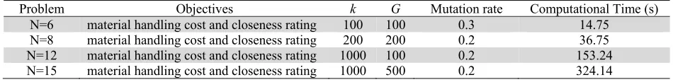
The specifications of FLPs are shown in Table 1. The problem size, objectives, fine-tuned parameter values of BBO algorithm and computational time required to run one trial of algorithm presented in Table 1. The parameters are finalised by taking number of trials to reach at optimum solutions. Table 2 shows the objective weights of all the problems determined by MWM, GMWM, SDWM and CRITICM methods explained in (Singh & Singh, 2010).

Table 1

Problem specification and BBO parameters setting

Problem Objectives k G Mutation rate Computational Time (s)

N=6 material handling cost and closeness rating 100 100 0.3 14.75

Table 2

Objective weights obtained using MWM, GMWM, SDWM and CRITICM

Problem MWM GMWM SDWM CRITICM

N = 6 (Rosenblatt, 1979) w1 = 0.5899

w2 =0.4101

w1 = 0.5036 w2 =0.4964

w1= 0.5051 w2 =0.4949

w1 = 0.5051 w2 =0.4949

N = 8 (Fortenberry and Cox, 1985) w1 = 0.5949

w2 = 0.4051

w1 = 0.4703 w2 = 0.5297

w1 = 0.5991 w2 = 0.4009

N = 12 (Dutta and Sahu, 1982) w1 = 0.6945

w2 =0.3055

w1 = 0.4693 w2 =0.5307

w1 = 0.5096 w2 =0.4904

N = 15 (Chen and Sha, 1999) w1 = 0.7448

w2 =0.2552

na w1 = 0.4566

w2 =0.5434

w1 = 0.4566 w2 =0.5434 The objective function value (OFV) using each weight method and the layout obtained using BBO algorithm is shown in Table 3. The best solutions are displayed in bold face. For N=8, BBO obtained two layouts using GMWM method which are shown in Table 3.

Fig. 3 Convergence of BBO for N= 6 FLP

From Table 3, it is seen that for problem size of 6, 8 and 12 the results obtained using BBO algorithm

are same as obtained by Matai (2015) and for size 15, BBO algorithm is giving better solutions in all the

21.85 21.9 21.95 22 22.05 22.1 22.15 22.2 22.25

1 5 9 ₁₃ ₁₇ ₂₁ ₂₅ ₂₉ ₃₃ ₃₇ ₄₁ ₄₅ ₄₉ ₅₃ ₅₇ ₆₁ ₆₅ ₆₉ ₇₃ ₇₇ ₈₁ ₈₅ ₈₉ ₉₃ ₉₇

101

Objective function

valu

e

Generations

(11)

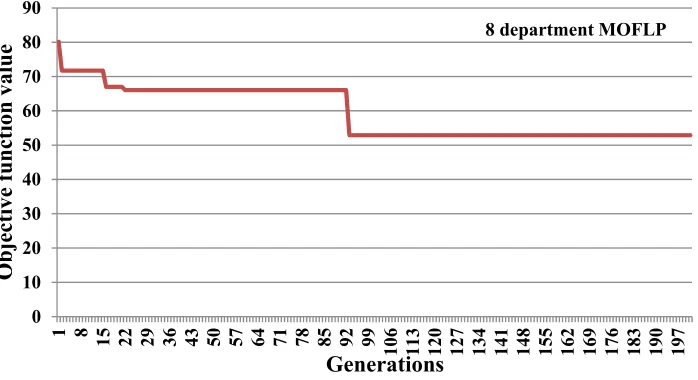
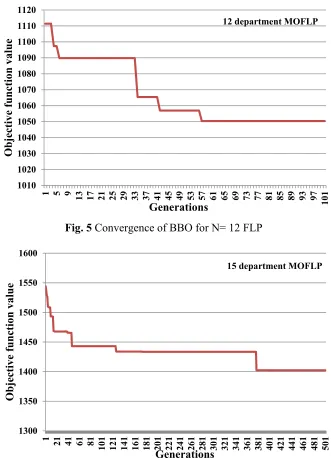
three methods. In 8-department FLP, two layouts are obtained for the same OFV. In Figs. 3-6, the graphs are plotted between generations and OFV which show the convergence nature of BBO algorithm. The algorithm is converging to near optimal solutions in minimum number of generations. This shows the capability of BBO algorithm to solve FLPs.

Table 3

Comparison of multi-objective FLPs with previous results

Problem Approach MWM GMWM SDWM CRITICM

N = 6 (Rosenblatt,

1979)

Singh and Singh (2010) 34.1759 [2-6-5-3-1-4] 22.0076 [2-6-5-3-1-4] 22.2191 [2-6-5-3-1-4] 22.2191 [2-6-5-3-1-4] Matai (2015) 34.1759

[4-3-1-5-6-2] 22.0076 [5-6-3-4-2-1] 22.2191 [4-3-1-5-6-2] 22.2191 [4-3-1-5-6-2]

BBO 34.1759

[2-6-5-3-1-4] 22.0076 [3-6-5-1-2-4] 22.2191 [5-6-2-4-3-1] 22.2191 [1-2-4-3-6-5] N = 8

(Fortenberry and Cox, 1985)

Singh and Singh (2010) 128.6624 [1-5-8-3-2-7-6-4] 105.78 [4-6-7-2-3-8-5-1] 127.256 [2-7-6-4-1-5-8-3] 127.256 [2-7-6-4-1-5-8-3] Matai (2015) 124.6624

[1-5-8-3-2-7-6-4] 52.8928 [4-6-7-2-3-8-5-1] 127.0816 [2-7-6-4-1-5-8-3] 127.0816 [2-7-6-4-1-5-8-3]

BBO 124.6624

[2-7-6-4-1-5-8-3] 52.8928 [1-5-8-3-2-7-6-4] [3-8-5-1-4-6-7-2] 127.0816 [3-8-5-1-4-6-7-2] 127.0816 [3-8-5-1-4-6-7-2]

N = 12 (Dutta and Sahu, 1982)

Singh and Singh (2010)

1766.99

[1-6-7-2-9-10-12-8-4-11-5-3]

1116.36 [4-6-

5-2-9-10-12-8-1-11-7-3]

1255.435 [4-6-

5-2-9-10-12-8-1-11-7-3]

1255.435 [4-6-

5-2-9-10-12-8-1-11-7-3] Matai (2015) 1678.2656

[3-5-12-2-8-7-10-6-1-11-9-4]

1050.4075 [3-5-

12-2-8-6-7-10-1-11-9-4]

1162.7645 [4-9-

11-1-10-7-6-8-2-12-5-3]

1162.7645 [4-9-

11-1-10-7-6-8-2-12-5-3] BBO 1678.2656

[4-9-11-1-10-7-6-8-2-12-5-3]

1050.4000 [2-

12-5-3-6-10-7-8-4-9-11-1]

1164.8000 [3-8-

11-1-12-5-6-7-2-10-9-4]

1164.8000 [3-8-

11-1-12-5-6-7-2-10-9-4] N = 15 (Chen

and Sha, 1999)

Singh and Singh (2010)

2701.64 [10-

12-1-13-6-15-14-8-2-11-4-7-9-3-5]

na 1557.68

[10-12-1-7-4-11-14-2-8-15-5-13-9-3-6]

1557.68 [10-

12-1-7-4-11-14-2-8-15-5-13-9-3-6] Matai (2015) 2459.5818

[12- 7-14-15-6-13-9-1-8-11-10-5-3-2-4]

na 1411.1108

[12-7-14-15-6-13-9-1-8-11-10-5-3-2-4]

1411.1108 [12-7-

14-15-6-13-9-1-8-11-10-5-3-2-4] BBO 2445.5000

[10-5-3-2-4-13-1- 14-8-11-12-9-7-15-6]

na 1402.4000

[10-5-3-2-4-13-1- 14-8-11-12-9-7-15-6]

1402.9000 [10- 3-1-2-4-13-5-14-8-11-12-9-7-15-6] 0 10 20 30 40 50 60 70 80 90

1 8 ₁₅ ₂₂ ₂₉ ₃₆ ₄₃ ₅₀ ₅₇ ₆₄ ₇₁ ₇₈ ₈₅ ₉₂ ₉₉

10 6 11 3 12 0 12 7 13 4 14 1 14 8 15 5 16 2 16 9 17 6 18 3 19 0 19 7 Ob jective fu nction value Generations

(12)

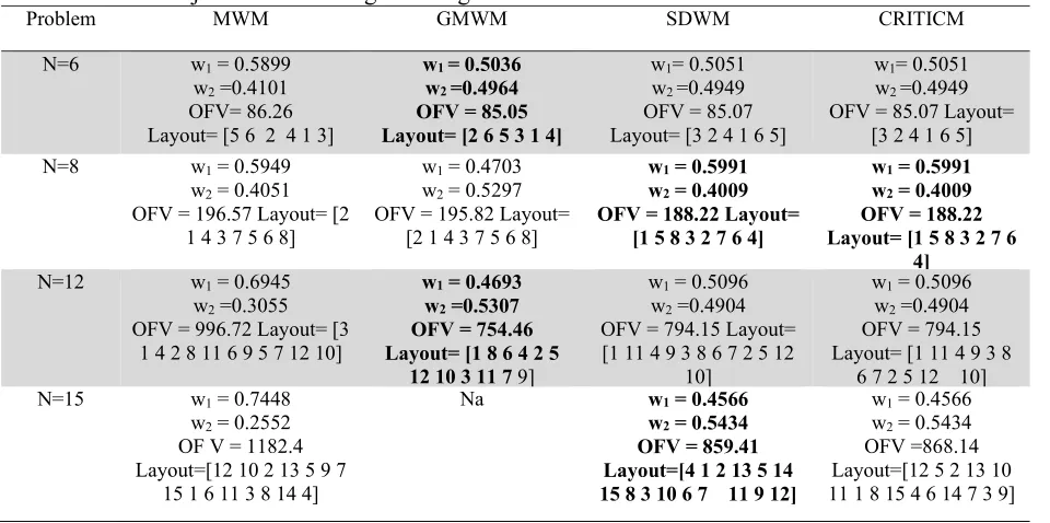
As we have earlier stated in section 3 about the objective functions; the results of multi-objective FLPs obtained using Eq. (4) and Eq. (5) are shown in Table 4. All the objective functions are evaluated separately to show the difference between the results. The comparison of original OFV obtained in this

work with that of Singh and Singh (2010) and Matai (2015)is given in Table 4. It is seen from Table 4

that the new values obtained from remodelled objective functions are different from original values. The results obtained for different objective weights are presented in Table 4 and these results cannot be

compared with the previous results due to the difference in second objective i.e. f2. The reason to show

the difference between the results obtained in this paper and results obtained by Singh and Singh (2010) and Matai (2015), is the correct values of the objective functions which should be considered as best layout by the layout planner.

1010 1020 1030 1040 1050 1060 1070 1080 1090 1100 1110 1120

1 5 9 ₁₃ ₁₇ ₂₁ ₂₅ ₂₉ ₃₃ ₃₇ ₄₁ ₄₅ ₄₉ ₅₃ ₅₇ ₆₁ ₆₅ ₆₉ ₇₃ ₇₇ ₈₁ ₈₅ ₈₉ ₉₃ ₉₇

10 1 Ob jective fu nction value Generations

12 department MOFLP

1300 1350 1400 1450 1500 1550 1600

1 ₂₁ ₄₁ ₆₁ ₈₁

10 1 12 1 14 1 16 1 18 1 20 1 22 1 24 1 26 1 28 1 30 1 32 1 34 1 36 1 38 1 40 1 42 1 44 1 46 1 48 1 50 1 Ob jective fu nction value Generations

(13)

Table 4

Results of multi-objective FLPs using BBO algorithm

Problem MWM GMWM SDWM CRITICM

N=6 w1 = 0.5899

w2 =0.4101 OFV= 86.26 Layout= [5 6 2 4 1 3]

w1 = 0.5036

w2 =0.4964

OFV = 85.05 Layout= [2 6 5 3 1 4]

w1= 0.5051 w2 =0.4949 OFV = 85.07 Layout= [3 2 4 1 6 5]

w1= 0.5051 w2 =0.4949 OFV = 85.07 Layout=

[3 2 4 1 6 5]

N=8 w1 = 0.5949

w2 = 0.4051 OFV = 196.57 Layout= [2

1 4 3 7 5 6 8]

w1 = 0.4703 w2 = 0.5297 OFV = 195.82 Layout=

[2 1 4 3 7 5 6 8]

w1 = 0.5991

w2 = 0.4009

OFV = 188.22 Layout= [1 5 8 3 2 7 6 4]

w1 = 0.5991

w2 = 0.4009

OFV = 188.22 Layout= [1 5 8 3 2 7 6

4]

N=12 w1 = 0.6945

w2 =0.3055 OFV = 996.72 Layout= [3

1 4 2 8 11 6 9 5 7 12 10]

w1 = 0.4693

w2 =0.5307

OFV = 754.46 Layout= [1 8 6 4 2 5

12 10 3 11 79]

w1 = 0.5096 w2 =0.4904 OFV = 794.15 Layout= [1 11 4 9 3 8 6 7 2 5 12

10]

w1 = 0.5096 w2 =0.4904 OFV = 794.15 Layout= [1 11 4 9 3 8

6 7 2 5 12 10]

N=15 w1 = 0.7448

w2 = 0.2552 OF V = 1182.4 Layout=[12 10 2 13 5 9 7

15 1 6 11 3 8 14 4]

Na w1 = 0.4566

w2 = 0.5434

OFV = 859.41 Layout=[4 1 2 13 5 14 15 8 3 10 6 7 11 9 12]

w1 = 0.4566 w2 = 0.5434 OFV =868.14 Layout=[12 5 2 13 10 11 1 8 15 4 6 14 7 3 9]

5.2 Performance evaluation of NSBBO algorithm

The multi-objective FLPs considered in this paper are not solved using Pareto-optimality method or non-dominance criteria in previous literature. In this section, NSBBO algorithm is applied to solve multi-objective FLPs. As we cannot compare the solutions obtained using weight approach with the solutions obtained using Pareto-optimality criteria, therefore both NSBBO and NSGA-II algorithms are implemented. The objective functions are described in previous section. In Pareto-optimality procedure the objective function are kept separate to obtain non-dominated solutions. The multi-objective FLP can be stated as:

, (18)

Eq. (18) indicates the functions of MHC and CR. In f2, which represents closeness rating score, is

considered as a penalty to be minimized (Sahin & Turkbey, 2009). The parameters of NSBBO and NSGA-II such as population or island size (P), generations (G), mutation rate and sharing fitness are decided by taking number of trials and kept same for both the algorithms. The values of these parameters are mentioned in Table 5.

Table 5

NSBBO and NSGA-II parameters setting

Problem P G Mutation rate Sharing fitness

N=6 100 100 0.15 1.3

N=8 100 150 0.15 1.2

N=12 200 500 0.20 1.2

N=15 200 1000 0.20 1.3

(14)

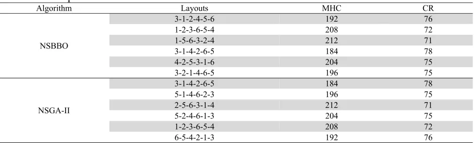
Table 6

Results of 6-department FLP

Algorithm Layouts MHC CR

NSBBO

3-1-2-4-5-6 192 76

1-2-3-6-5-4 208 72

1-5-6-3-2-4 212 71

3-1-4-2-6-5 184 78

4-2-5-3-1-6 204 75

3-2-1-4-6-5 196 75

NSGA-II

3-1-4-2-6-5 184 78

5-1-4-6-2-3 196 75

2-5-6-3-1-4 212 71

5-2-4-6-1-3 204 75

1-2-3-6-5-4 208 72

6-5-4-2-1-3 192 76

The results of 6-department FLP using NSBBO and NSGA-II are shown in Table 6. This problem is

small in size; therefore best solutions are obtained from both the algorithms. Each method has provided 6 solutions with different layouts. Therefore, the layout planner can decide the layout according to his/her preference. Pareto solutions and efficient frontier of 6-department FLP for NSBBO and NSGA-II are shown in Fig. 7 and Fig. 8, respectively. It is seen that both the frontier are same.

Fig. 7. Pareto solution front of 6-department FLP using NSBBO

Fig. 8. Pareto solution front of 6-department FLP using NSGA-II

70 71 72 73 74 75 76 77 78 79

180 185 190 195 200 205 210 215

Closeness rati

ng

Material handling cost

NSBBO

70 71 72 73 74 75 76 77 78 79

180 185 190 195 200 205 210 215

C

lo

se

n

es

s ra

ti

ng

(15)

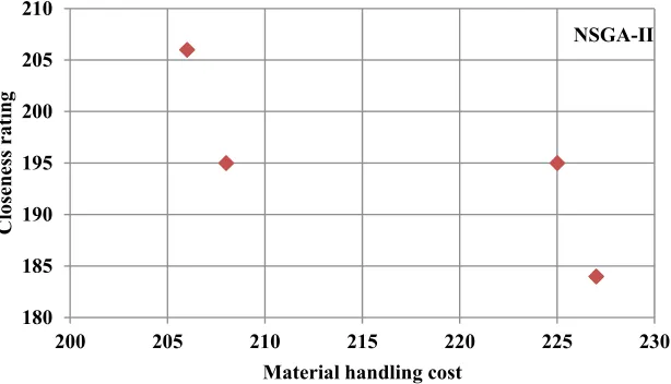
Table 7 shows the results of 8-department problem using NSBBO and NSGA-II methods. NSBBO algorithm has provided five non-dominated solutions while NSGA-II has provided four solutions of MHC and CR.

Table 7

NSBBO

7-5-8-4-2-1-6-3 206 206

4-6-5-8-2-7-1-3 210 203

3-8-5-1-4-7-6-2 203 208

6-7-1-4-8-5-2-3 228 182

3-6-8-2-4-7-5-1 202 212

NSGA-II

2-4-1-3-7-6-5-8 208 195

2-1-5-7-3-4-6-8 225 195

2-1-8-3-7-6-5-4 206 206

2-1-7-6-4-3-5-8 227 184

Fig. 9 and Fig. 10 show that Pareto frontiers of NSBBO and NSGA-II respectively for 8-department problem.

Fig. 9. Pareto solution front of 8-department FLP using NSBBO

180 185 190 195 200 205 210 215

200 205 210 215 220 225 230

Clos

eness rat

ing

NSBBO

180 185 190 195 200 205 210

200 205 210 215 220 225 230

Cl

oseness rati

ng

(16)

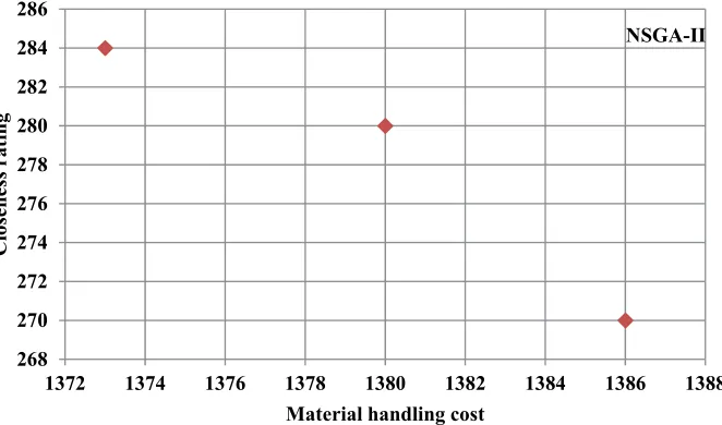
In Table 8, results of 12-department problem are presented. NSBBO has provided four non-dominated solutions while II has provided three solutions. Efficient Pareto frontier of NSBBO and NSGA-II for 12-department MOFLP are shown in Fig. 11 and Fig. 12, respectively.

Table 8

NSBBO

4-10-5-11-9-12-7-8-2-1-6-3 1334 307

10-8-7-4-12-5-6-3-9-2-11-1 1380 265

1-4-7-6-10-9-12-8-2-11-5-3 1322 314

2-7-9-4-1-11-8-6-3-12-5-10 1367 304

NSGA-II

4-1-3-2-6-5-11-8-7-9-12-10 1386 270

1-2-3-4-5-12-6-11-8-10-7-9 1380 280

1-2-3-8-9-11-5-10-4-7-6-12 1373 284

Fig. 11 Pareto solution front of 12-department FLP using NSBBO

Fig. 12 Pareto solution front of 12-department FLP using NSGA-II

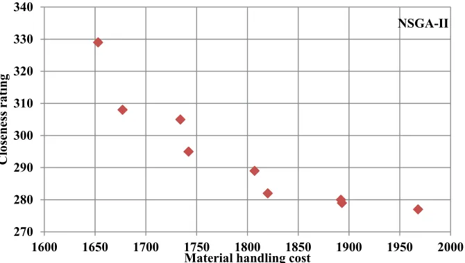
Table 9 shows the Pareto solutions of 15-department FLP. NSBBO provided 6 solutions while NSGA-II provided 9 solutions. The Pareto curves of NSBBO and NSGA-II for 15-department problem are shown in Fig. 13 and Fig.14, respectively.

260 270 280 290 300 310 320

1310 1320 1330 1340 1350 1360 1370 1380 1390

Cl

oseness r

ating

NSBB

268 270 272 274 276 278 280 282 284 286

1372 1374 1376 1378 1380 1382 1384 1386 1388

Closene

ss rating

(17)

Table 9

NSBBO

13-7-6-2-4-3-5-10-8-1-11-12-14-15-9 1886 280

4-7-12-10-5-9-3-13-2-1-6-15-8-11-14 1624 318

2-14-8-4-11-12-1-7-6-9-5-10-13-15-3 1617 357

5-10-12-6-11-2-8-14-1-9-3-13-7-15-4 1667 302

4-13-1-6-11-12-15-8-2-3-7-9-14-5-10 1693 298

6-5-1-4-10-14-11-3-13-9-12-8-2-7-15 1714 285

NSGA-II

14-1-11-8-2-3-4-7-12-5-6-9-13-10-15 1734 305

7-4-1-2-3-9-13-8-5-12-6-10-15-14-11 1807 289

7-15-1-2-12-4-13-8-3-5-9-10-11-6-14 1820 282

5-4-2-15-1-3-10-8-7-6-13-9-12-11-14 1677 308

1-2-5-7-3-4-10-11-6-14-9-8-15-13-12 1968 277

6-2-1-7-4-3-5-10-8-9-11-13-14-12-15 1893 279

5-3-1-4-9-2-14-8-11-7-6-13-15-10-12 1742 295

4-1-3-8-2-6-11-15-7-5-14-13-9-12-10 1653 329

1-2-3-5-11-4-13-6-7-8-9-10-15-14-12 1892 280

Fig. 13. Pareto solution front of 15-department FLP using NSBBO

0 50 100 150 200 250 300 350 400

1600 1650 1700 1750 1800 1850 1900

C

lo

se

n

es

s ra

ti

ng

NSBBO

270 280 290 300 310 320 330 340

1600 1650 1700 1750 1800 1850 1900 1950 2000

Cl

os

eness rati

ng

(18)

All the 15 solutions obtained are non-comparable and considered as equally good. This gives flexibility to the layout planner to select appropriate layout considering other criteria as per requirement. The overall performance of both BBO and NSBBO algorithms show their applicability on complex combinatorial problems of multi-objective FLPs.

6. Conclusion

In this paper, BBO meta-heuristic algorithm has been employed to solve complex multi-objective FLPs, which are otherwise very difficult to solve using traditional techniques. Both weight approach and Pareto-optimality approach were considered to obtain better results. The results obtained using BBO algorithm (weight approach) for 6, 8, 12 and 15 departments FLP are better or equal as compared to previous results. Furthermore, NSBBO algorithm was proposed to find Pareto-optimal solutions of FLPs. The solutions are non-dominated which are not biased to any one objective. The comparison of NSBBO and NSGA-II is proving that NSBBO is performing as good as NSGA-II. The layout planner can decide best layout among number of solutions according to his/her preference.

The computational time required to run BBO algorithm is satisfactory. This makes BBO algorithm efficient to solve combinatorial optimization problems like FLP. An important observation regarding objective functions of FLP is discussed and remodelled functions are evaluated to show the difference between the final solutions. The distance between the departments should be incorporated while considering the objectives related to movement of material. As BBO and NSBBO algorithms are capable to solve multi-objective FLPs, it can be further implemented to solve multi-objective, dynamic and unequal area FLPs.

References

Aiello, G., Scalia, G. L. & Enea, M. (2012). A multi objective genetic algorithm for the facility layout

problem based upon slicing structure encoding. Expert Systems with Applications,39, 10352–10358.

Aiello, A., LaScalia, G. & Enea, M. (2013). A non-dominated ranking multi objective Genetic Algorithm

& electre method for unequal area facility layout problems. Expert Systems with Applications, 40,

4812–4819.

Alroomi, A. R., Albasri, F. A. & Talaq, J. H. (2013). Essential modifications on Biogeography-based

optimization algorithm. Computer Science & Information Technology, 141-160. doi:

10.5121/csit.2013.3812

Chen, G. Y. & Lo, J. (2014). Dynamic facility layout with multi-objectives. Asia-pacific Journal of

Operation Research,31(4), 1450027. doi: 10.1142/s0217595914500274

Chen, C.W. & Sha, D.Y. (1999). A design approach to the multi-objective facility layout problem.

International journal of production research, 37(5), 1175- 1196.

Chen, C.W. & Sha, D.Y. (2005). Heuristic approach for solving the multi-objective facility layout

problem. International Journal of Production Research, 43(21), 4493–4507.

Chiang, W. C., Kouvelis, P. & Urban, T. L. (2006). Single- & multi-objective facility layout with

workflow interference considerations. European Journal of Operational Research, 174, 1414–1426.

Chutima, P. & Naruemitwong, W. (2014). A Pareto biogeography-based optimisation for multi-objective

two-sided assembly line sequencing problems with a learning effect. Computers & Industrial

Engineering, 69, 89–104.

Deb, K., Pratap, A., Agarwal, S. & Meyarivan, T. (2002). A fast & elitist multi-objective genetic

algorithm: NSGA-II. IEEE Transactions on Evolutionary Computation, 6(2), 82–197.

Dutta, K. N. & Sahu, S. (1982). A multigoal heuristic for facilities design problems: MUGHAL.

International Journal of Production Research,20(2), 147-154.

Fortenberry, J. C. & Cox, J. F. (1985). Multiple criteria approach to the facilities layout problem.

(19)

Harmonosky, C. M. & Tothero, G. K., (1992). A multi-factor plant layout methodology. International

Journal of Production Research, 30, 1773–1789.

Hathhorn, J., Sisikoglu, H. & Mustafa Y. (2013). A multi-objective mixed-integer programming model

for a multi-floor facility layout. International Journal of Production Research, 51(14), 4223–4239.

Jolai, F., Moghaddam, R.T. & Taghipour, M. (2012). A multi-objective particle swarm optimisation

algorithm for unequal sized dynamic facility layout problem with pickup/drop-off locations.

International Journal of Production Research, 50(15), 4279–4293.

Khare, V. K., Khare, M. K. & Neema, M. L. (1988). Combined computer-aided approach for the facilities design problem & estimation of the distribution parameter in the case of multi-goal optimization.

Computers & Industrial Engineering, 14(4), 465-476.

Ku, M.Y., Hu, M. H. & Wang, M. J. (2011).Simulated annealing based parallel genetic algorithm for

facility layout problem. International Journal of Production Research, 49 (6), 1801–1812.

Lim, W. L., Wibowo, A., Desa, M. I. & Haron, H. (2016). A biogeography-based optimization algorithm

hybridized with tabu search for the quadratic assignment problem. Computational Intelligence &

Neuroscience, Article ID 5803893. doi: org/10.1155/2016/5803893

Ma, H., Ruan, X., & Pan, Z. (2012). H&ling multiple objectives with biogeography-based Optimization.

International Journal of Automation & Computing, 9(1), 30-36.

Ma, H., Su, S., Simon, D. & Fei, M. (2015). Ensemble multi-objective biogeography-based optimization

with application to automated warehouse scheduling. Engineering Applications of Artificial

Intelligence, 44, 79–90.

Matai, R., Singh, S.P. & Mittal, M.L. (2013). Modified simulated annealing based approach for multi

objective facility layout problem. International Journal of Production Research, 51(14), 4273–4288.

Matai, R. (2015). Solving multi objective facility layout problem by modified simulated annealing.

Applied Mathematics & Computation,261, 302–311.

Peer, S. K. & Sharma, D. K. (2008).Human–computer interaction design with multi-goal facilities layout

model. Computers & Mathematics with Applications, 56, 2164–2174.

Rahmati, S. A. & Zandieh, M. (2012). A new biogeography-based optimization (BBO) algorithm for the

flexible job shop scheduling problem. International Journal of Advanced Manufacturing Technology,

58, 1115–1129.

Ripon, K. S. N., Glette, K., Khan, K. N., Hovin, M. & Torresen, J. (2013). Adaptive variable neighbourhood search for solving multi-objective facility layout problems with unequal area facilities.

Swarm & Evolutionary Computation,8, 1–12

Rosenblatt, J. M. (1979). The facilities layout problem: A multi-goal approach. International Journal of

Production Research,17(4), 323–332.

Sahin, R. & Turkbey, O. (2009). A simulated annealing algorithm to find approximate Pareto optimal

solutions for the multi-objective facility layout problem. International Journal of Advanced

Manufacturing Technology,41, 1003–1018.

Sahin , R. (2011). A simulated annealing algorithm for solving the bi-objective facility layout problem.

Expert Systems with Applications, 38, 4460–4465.

Simon, D. (2008). Biogeography-based optimization. IEEE Transactions on Evolutionary Computation,

12(6), 702-713.

Simon, D. (2013). Evolutionary Optimization Algorithms. John Wiley & Sons, Hoboken, NJ.

Singh, S. P. & Singh, V. K. (2010). An improved heuristic approach for multi-objective facility layout

problem. International Journal of Production Research, 48(4), 1171–1194.

Sooncharoen, S., Vitayasak, S., & Pongcharoen, P. (2015). Application of biogeography-based

optimisation for machine layout design problem. International Journal of Mechanical Engineering &

Robotic Research, 4(3), 251-254.

Urban, T. L. (1987). A multiple criteria model for the facilities layout problem. International Journal of

Production Research, 25(12), 1805-1812.

Ye, M., & Zhou, G. (2007). A local genetic approach to multi-objective, facility layout problems with

(20)

Zhou, X., Liu, Y., Li, B. & Sun, G. (2015). Multi-objective biogeography based optimization algorithm

with decomposition for community detection in dynamic networks. Physica A: Statistical Mechanics

& its Applications, 436, 430–442.

Appendix A

A.1 Demonstration steps of BBO algorithm with an illustrative example of n=5 department

problem

Step 1: Randomly generate islands (k = 5). Each layout is considered as one island. Since there are 5 departments, string length of each island consists of 5 random numbers.

{0.8147 0.0975 0.1576 0.1419 0.6557} {0.9058 0.2785 0.9706 0.4218 0.0357} {0.1270 0.5469 0.9572 0.9157 0.8491} {0.9134 0.9575 0.4854 0.7922 0.9340} {0.6324 0.9649 0.8003 0.9595 0.6787}

Step 2: Obtain the integer numbers for departments by sorting and indexing each row of above matrix. Evaluate OFV of each layout.

L1 : 2 – 4 – 3 – 5 – 1; OFV: 186 L2 : 5 – 2 – 4 – 1 – 3; OFV: 168 L3 : 1 – 2 – 5 – 4 – 3; OFV: 179 L4 : 3 – 4 – 1 – 5 – 2; OFV: 151 L5 : 1 – 5 – 3 – 4 – 2; OFV: 163

From initial layouts, the minimum OFV is 151 and the corresponding layout is the best layout.

Step 3: Start first iteration. The emigration rate μs and immigration rate λs are calculated using Eqs. (11) and (12) respectively.

μs = {0.2, 0.4, 0.6, 0.8, 1}

λs = {0.8, 0.6, 0.4, 0.2, 0}

Probability of the species Ps is calculated using Eq. (13)

Ps = {0.0313, 0.1563, 0.3125, 0.3125, 0.1563, 0.0313 }

Step 4: Start migration operation. Select two islands for emigration and immigration. Using μs, fourth

island is selected for emigration and using λs, first island is selected for immigration. Randomly select

SIVs from fourth and first island to replace their positions. Suppose fifth and second SIVs are selected from fourth and first island respectively and their positions are replaced. The numbers replaced are shown in bold. The new islands will be as follows:

{0.8147 0.9340 0.1576 0.1419 0.6557}

{0.9058 0.2785 0.9706 0.4218 0.0357} {0.1270 0.5469 0.9572 0.9157 0.8491}

{0.9134 0.9575 0.4854 0.7922 0.0975}

{0.6324 0.9649 0.8003 0.9595 0.6787}

Step 5: Start mutation operation. The mutation rate is calculated using Eq. (17). m = {0.8998, 0.4998, 0, 0, 0.4998, 0.8998}

Using Ps, two islands are selected. In each island, one SIV is selected to replace with randomly generated

number. Suppose first and fifth islands are selected for mutation. From first island, third SIV is selected

and from fifth island, fourth SIV is selected to replace with random numbers r1 = 0.3781and r2 = 0.4424,

respectively. After mutation the islands obtained are

(21)

D. Singh and S. Ingole / International Journal of Industrial Engineering Computations 10 (2019) {0.9058 0.2785 0.9706 0.4218 0.0357} {0.1270 0.5469 0.9572 0.9157 0.8491} {0.9134 0.9575 0.4854 0.7922 0.0975} {0.6324 0.9649 0.8003 0.4424 0.6787}

Again find the integer numbers by sorting and indexing each row of above matrix to get the layouts and their OFVs after mutation.

L1 : 4 – 3 – 5 – 1 – 2; OFV: 166 L2 : 5 – 2 – 4 – 1 – 3; OFV: 168 L3 : 1 – 2 – 5 – 4 – 3; OFV: 179 L4 : 5 – 3 – 4 – 1 – 2; OFV: 172 L5 : 4 – 1 – 5 – 3 – 2; OFV: 148

Step 7: After first iteration, the best layout and its OFV obtained is: 4 – 1 – 5 – 3 – 2; OFV = 148

Step 8: Repeat steps 3 to 7 until maximum number of iterations is reached.

A.2 Demonstration steps of NSBBO with an illustrative example of 8 departments.

Step 1. Generate initial islands/population (P=10) of random numbers. Set the values of

iterations/generations (G), mutation rate, sharing fitness (σshare) and dummy fitness. The random numbers

are indexed and sorted to obtain layouts. Calculate both the objectives of material handling cost (MHC) and closeness rating (CR) for each layout.

Sr.

No. Randomly generated islands Layout MHC CR

1 0.7772 0.6679 0.0615 0.7989 0.1103 0.9705 0.0866 0.1006 3 7 8 5 2 1 4 6 244 212

2 0.9051 0.6034 0.7801 0.7343 0.1174 0.8669 0.7719 0.2940 5 8 2 4 7 3 6 1 247 227

3 0.5337 0.5261 0.3375 0.0513 0.6407 0.0862 0.2056 0.2373 4 6 7 8 3 2 1 5 226 198

4 0.1091 0.7297 0.6078 0.0728 0.3288 0.3664 0.3882 0.5308 4 1 5 6 7 8 3 2 269 237

5 0.8258 0.7072 0.7412 0.0885 0.6538 0.3691 0.5517 0.0914 4 8 6 7 5 2 3 1 261 234

6 0.3380 0.7813 0.1048 0.7983 0.7491 0.6850 0.2289 0.4053 3 7 1 8 6 5 2 4 264 226

7 0.2939 0.2879 0.1278 0.9430 0.5831 0.5979 0.6419 0.1048 8 3 2 1 5 6 7 4 232 210

8 0.7463 0.6925 0.5495 0.6837 0.7400 0.7893 0.4844 0.1122 8 7 3 4 2 5 1 6 243 216

9 0.0103 0.5566 0.4852 0.1320 0.2348 0.3676 0.1518 0.7844 1 4 7 5 6 3 2 8 252 218

10 0.0484 0.3965 0.8904 0.7227 0.7349 0.2060 0.7819 0.2915 1 6 8 2 4 5 7 3 241 221

Step 2: Start first iteration. Rank the objectives according to non-dominated solutions as shown below:

Rank Layouts Islands MHC CR

(22)

Step 3. Calculate shared fitness, niche count and dummy fitness using Eqs.8-10 respectively. Calculate probability and cumulative probability for selection of islands.

Sr. No. Niche count Dummy fitness Shared fitness Probability Cumulative probability

1 1.2 50.0000 41.6666 0.3949 0.3949

2 1.2 41.5631 34.6359 0.3282 0.7232

3 4.2 34.1715 8.1360 0.0771 0.8003

4 4.2 34.1715 8.1360 0.0771 0.8774

5 4.2 34.1715 8.1360 0.0771 0.9545

6 4.2 8.0685 1.9210 0.0182 0.9727

7 4.2 8.0685 1.9210 0.0182 0.9910

8 4.2 1.7263 0.4110 0.0038 0.9948

9 4.2 1.7263 0.4110 0.0038 0.9987

10 1.2 0.1529 0.1274 0.0012 1.0000

Step 4: Generate random number for each member and sort the islands with respect to probability and cumulative probability.

Rand no. Sorted Islands sorted with respect to cumulative probability and random no.

0.6554 2 0.2939 0.2879 0.1278 0.9430 0.5831 0.5979 0.6419 0.1048

0.1097 4 0.7463 0.6925 0.5495 0.6837 0.7400 0.7893 0.4844 0.1122

0.9337 5 0.0484 0.3965 0.8904 0.7227 0.7349 0.2060 0.7819 0.2915

0.1874 10 0.1091 0.7297 0.6078 0.0728 0.3288 0.3664 0.3882 0.5308

0.2661 9 0.3380 0.7813 0.1048 0.7983 0.7491 0.6850 0.2289 0.4053

0.7978 7 0.0103 0.5566 0.4852 0.1320 0.2348 0.3676 0.1518 0.7844

0.4876 1 0.5337 0.5261 0.3375 0.0513 0.6407 0.0862 0.2056 0.2373

0.7689 8 0.8258 0.7072 0.7412 0.0885 0.6538 0.3691 0.5517 0.0914

0.3960 6 0.9051 0.6034 0.7801 0.7343 0.1174 0.8669 0.7719 0.2940

0.2729 3 0.7772 0.6679 0.0615 0.7989 0.1103 0.9705 0.0866 0.1006

Step 5: Apply migration operator to the islands by using migration probability. Mutation is done by using mutation probability. The updated islands are given below:

Sr. No. Islands after migration Islands after mutation

1 0.2939 0.2879 0.1278 0.9430 0.5831 0.5979 0.6419 0.1048 0.2939 0.2879 0.1278 0.9430 0.5831 0.5979 0.6419 0.1048

2 0.7463 0.6925 0.5495 0.6837 0.7400 0.7893 0.4844 0.1122 0.7463 0.6925 0.5495 0.6837 0.7400 0.7893 0.4844 0.1122

3 0.0484 0.3965 0.8904 0.0728 0.5831 0.2060 0.7819 0.2915 0.0484 0.3965 0.8904 0.0728 0.5831 0.2060 0.7819 0.2915

4 0.1091 0.7297 0.6078 0.7983 0.2348 0.6850 0.3882 0.5308 0.1091 0.7297 0.6078 0.7983 0.2348 0.6850 0.3882 0.5308

5 0.0484 0.7813 0.1048 0.7983 0.2348 0.6850 0.2289 0.4053 0.0484 0.7813 0.1048 0.7983 0.2348 0.6850 0.2289 0.4053

6 0.0103 0.6679 0.7412 0.1320 0.1174 0.3676 0.7719 0.0914 0.0103 0.6679 0.7412 0.1320 0.1174 0.3676 0.7719 0.0914

7 0.0103 0.5261 0.7412 0.0513 0.6407 0.7893 0.7719 0.1006 0.0103 0.5261 0.7412 0.0513 0.6407 0.7893 0.7719 0.1006

8 0.9051 0.6034 0.8904 0.0513 0.5831 0.3691 0.3882 0.1006 0.9051 1.5346 0.8904 0.0513 0.5831 0.3691 0.3882 0.1006

9 0.9051 0.6034 0.7801 0.7343 0.1174 0.8669 0.7719 0.2940 0.9051 0.6034 0.7801 0.7343 0.1174 0.8669 0.7719 0.2940 10 0.7772 0.6679 0.0615 0.7989 0.1103 0.9705 0.0866 0.1006 0.8667 0.6679 0.0615 0.7989 0.1103 0.9705 0.0866 0.1006

Step 6: Evaluate the objective function values after first iteration as follows:

Sr. No. Layouts MHC CR

1 8 3 2 1 5 6 7 4 232 210

2 8 7 3 4 2 5 1 6 243 216

3 1 4 6 8 2 5 7 3 220 216

4 1 5 7 8 3 6 2 4 250 215

5 1 3 7 5 8 6 2 4 254 231

6 1 8 5 4 6 2 3 7 256 233

7 1 4 8 2 5 3 7 6 252 222

8 4 8 6 7 5 3 1 2 234 219

9 5 8 2 4 7 3 6 1 247 227

10 3 7 8 5 2 4 1 6 244 207

Step 7: The non-dominated solutions after first iteration are given below:

Sr. No. Layouts MHC CR

1 1 3 7 5 8 6 2 4 254 231

(23)

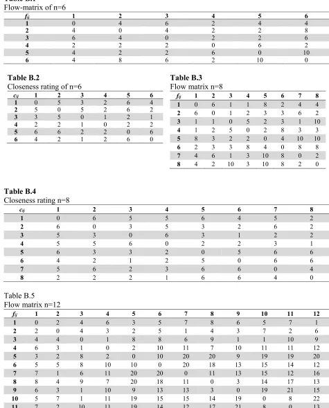
Appendix B: Tables B.1 – B.8 shows the material flow and closeness rating for multi-objective FLPs.

Table B.1

Flow-matrix of n=6

fij 1 2 3 4 5 6

1 0 4 6 2 4 4

2 4 0 4 2 2 8

3 6 4 0 2 2 6

4 2 2 2 0 6 2

5 4 2 2 6 0 10

6 4 8 6 2 10 0

Table B.2

Closeness rating of n=6

cij 1 2 3 4 5 6

1 0 5 3 2 6 4

2 5 0 5 2 6 2

3 3 5 0 1 2 1

4 2 2 1 0 2 2

5 6 6 2 2 0 6

6 4 2 1 2 6 0

Table B.3

Flow matrix n=8

fij 1 2 3 4 5 6 7 8

1 0 6 1 1 8 2 4 4

2 6 0 1 2 3 3 6 2

3 1 1 0 5 2 3 1 10

4 1 2 5 0 2 8 3 3

5 8 3 2 2 0 4 10 10

6 2 3 3 8 4 0 8 8

7 4 6 1 3 10 8 0 2

8 4 2 10 3 10 8 2 0

Table B.4

Closeness rating n=8

cij 1 2 3 4 5 6 7 8

1 0 6 5 5 6 4 5 2

2 6 0 3 5 3 2 6 2

3 5 3 0 6 3 1 2 2

4 5 5 6 0 2 2 3 1

5 6 3 3 2 0 5 6 6

6 4 2 1 2 5 0 6 6

7 5 6 2 3 6 6 0 4

8 2 2 2 1 6 6 4 0

Table B.5

Flow matrix n=12

fij 1 2 3 4 5 6 7 8 9 10 11 12

1 0 2 4 6 3 5 7 8 6 5 7 1

2 2 0 4 3 2 5 1 4 3 7 2 6

3 4 4 0 1 8 8 6 9 1 1 10 9

4 6 3 1 0 2 10 11 7 10 11 11 12

5 3 2 8 2 0 10 20 20 9 19 19 20

6 5 5 8 10 10 0 20 18 13 15 14 12

7 7 1 6 11 20 20 0 11 13 15 12 16

8 8 4 9 7 20 18 11 0 3 14 17 13

9 6 3 1 10 9 13 13 3 0 19 21 15

10 5 7 1 11 19 15 15 14 19 0 8 22

11 7 2 10 11 19 14 12 17 21 8 0 13

(24)

Table B.6

cij 1 2 3 4 5 6 7 8 9 10 11 12

1 0 5 4 1 1 1 1 1 -1 1 2 2

2 5 0 3 1 4 4 1 5 1 3 2 2

3 4 3 0 3 1 1 1 1 -1 1 2 2

4 1 1 3 0 4 3 3 3 1 1 2 2

5 1 4 1 4 0 5 4 1 1 1 2 2

6 1 4 1 3 5 0 5 1 1 1 2 2

7 1 1 1 3 4 5 0 1 1 1 2 2

8 1 5 1 3 1 1 1 0 1 4 2 2

9 -1 1 -1 1 1 1 1 1 0 1 2 2

10 1 3 1 1 1 1 1 4 1 0 2 2

11 2 2 2 2 2 2 2 2 2 2 0 2

12 2 2 2 2 2 2 2 2 2 2 2 0

Table B.7

Flow matrix n=15

fij 1 2 3 4 5 6 7 8 9 10 11 12 13 14 15

1 0 4 5 8 12 16 3 7 2 6 8 9 12 17 12

2 15 0 6 8 12 0 9 35 4 7 3 6 9 8 12

3 15 16 0 9 2 0 15 6 17 6 12 3 5 8 9

4 1 25 9 0 2 6 5 8 0 0 0 0 3 2 9

5 5 0 15 6 0 2 0 8 0 9 0 6 6 3 2

6 8 5 0 6 9 0 5 8 8 0 6 0 3 5 8

7 0 3 5 0 8 9 0 9 9 8 7 12 0 13 15

8 16 17 0 16 15 11 14 0 1 4 12 2 15 15 13

9 17 6 9 11 25 6 12 12 0 5 7 8 9 2 6

10 3 8 9 6 0 0 0 0 0 0 0 5 6 0 7

11 8 9 0 12 15 16 0 0 2 4 0 5 0 5 7

12 6 7 2 8 9 12 15 5 5 0 0 0 7 0 5

13 6 4 3 8 9 0 11 5 15 15 10 10 0 5 10

14 12 6 9 8 10 11 15 5 16 12 10 10 5 0 7

15 2 3 4 8 0 12 15 16 12 0 0 0 0 2 0

Table B.8

cij 1 2 3 4 5 6 7 8 9 10 11 12 13 14 15

1 0 2 0 3 0 -1 2 0 3 1 4 -1 2 2 0

2 2 0 3 1 2 3 2 4 0 3 0 1 1 0 1

3 0 3 0 0 3 1 0 2 -1 0 4 0 2 1 0

4 3 1 0 0 -1 0 1 0 4 4 0 1 2 0 2

5 0 2 3 -1 0 0 1 3 0 2 1 0 1 0 0

6 -1 3 1 0 0 0 2 0 0 3 0 1 3 3 0

7 2 2 0 1 1 2 0 0 0 0 -1 2 1 0 1

8 0 4 2 0 3 0 0 0 1 4 3 2 3 3 2

9 3 0 -1 4 0 0 0 1 0 3 0 2 1 0 3

10 1 3 0 4 2 3 0 4 3 0 1 0 1 0 1

11 4 0 4 0 1 0 -1 3 0 1 0 3 2 1 1

12 -1 1 0 1 0 1 2 2 2 0 3 0 -1 1 1

13 2 1 2 2 1 3 1 3 1 1 2 -1 0 0 1

14 2 0 1 0 0 3 0 3 0 0 1 1 0 0 0

15 0 1 0 2 0 0 1 2 3 1 1 1 1 0 0