www.solid-earth.net/6/33/2015/ doi:10.5194/se-6-33-2015
© Author(s) 2015. CC Attribution 3.0 License.
Finite-difference modelling to evaluate seismic P-wave and
shear-wave field data
T. Burschil, T. Beilecke, and C. M. Krawczyk
Leibniz Institute for Applied Geophysics, Stilleweg 2, 30655 Hannover, Germany
Correspondence to: T. Burschil ([email protected])
Received: 16 July 2014 – Published in Solid Earth Discuss.: 1 August 2014
Revised: 12 November 2014 – Accepted: 14 November 2014 – Published: 13 January 2015
Abstract. High-resolution reflection seismic methods are an established non-destructive tool for engineering tasks. In the near surface, shear-wave reflection seismic measurements usually offer a higher spatial resolution in the same effective signal frequency spectrum than P-wave data, but data quality varies more strongly.
To discuss the causes of these differences, we investigated a P-wave and a SH-wave seismic reflection profile mea-sured at the same location on the island of Föhr, Germany and applied seismic reflection processing to the field data as well as finite-difference modelling of the seismic wave field. The simulations calculated were adapted to the acquisition field geometry, comprising 2 m receiver distance (1 m for SH wave) and 4 m shot distance along the 1.5 km long P-wave and 800 m long SH-wave profiles. A Ricker wavelet and the use of absorbing frames were first-order model parameters. The petrophysical parameters to populate the structural mod-els down to 400 m depth were taken from borehole data, VSP (vertical seismic profile) measurements and cross-plot rela-tions.
The simulation of the P-wave wave-field was based on in-terpretation of the P-wave depth section that included a priori information from boreholes and airborne electromagnetics. Velocities for 14 layers in the model were derived from the analysis of five nearby VSPs (vP=1600–2300 m s−1). Syn-thetic shot data were compared with the field data and seis-mic sections were created. Major features like direct wave and reflections are imaged. We reproduce the mayor reflec-tors in the depth section of the field data, e.g. a prominent till layer and several deep reflectors. The SH-wave model was adapted accordingly but only led to minor correlation with the field data and produced a higher signal-to-noise ra-tio. Therefore, we suggest to consider for future simulations
additional features like intrinsic damping, thin layering, or a near-surface weathering layer. These may lead to a better understanding of key parameters determining the data quality of near-surface shear-wave seismic measurements.
1 Introduction
Near-surface geophysical methods constitute a non-destructive means to investigate the shallow subsurface. Especially engineering tasks, for instance geohazard assess-ment or groundwater prospecting, profit from structural and parametrical methods (e.g. Miller, 2013; Kirsch, 2008). In some cases, results of geophysical prospecting are compiled into 3-D models and can act as input for, e.g. groundwater flow modelling.
structures is finite-difference (FD) modelling (Alterman and Karal, 1968). The advantage of the FD method is the ability to choose arbitrary heterogeneous input models without fun-damental restrictions. Drawbacks like high-computational requirements have become less restricting during the past years. The FD code by Bohlen (2002) has the ability to in-clude intrinsic seismic wave absorption, an advantage with respect to the study of unconsolidated material.
Full waveform inversion with either synthetic or real field data is an evolving field in exploration seismology. It aims at the automatic subsurface model generation from seismic field data. Although there has been a lot of progress in its evolution, and it can be applied routinely for simple subsur-face structures, especially in marine environments, its appli-cation for near-surface studies is still experimental (Romd-hane et al., 2011; Groos et al., 2012; Plessix, 2012). This has to do with the importance of a good starting model for the inversion process but also with the large parameter space in the near surface. Also, many seismic surveys try to avoid low frequencies in order to not generate large surface waves. Yet, the low frequencies are an important prerequisite to find the global optimum in the optimization process of the inversion (e.g. Virieux and Operto, 2009; Fichtner et al., 2011). There-fore, we focus here on direct modelling.
In this paper we describe the acquisition and processing of P-wave and SH-wave reflection seismic field data along an example profile. We generated synthetic P-wave data of the same profile with a FD algorithm on the basis of the P-wave depth section interpreted with a priori geological and geophysical information. The synthetic data were compared with the field data. Main reflectors can be reproduced. To assess the lower signal-to-noise ratio of the recorded shear-wave field data, we simulated SH-shear-wave seismograms on the basis of this model to comprehend quality variations in the SH-wave reflection field data.
2 Finite-difference modelling
Seismic wave-field modelling reveals the propagation of seis-mic waves within a subsurface model. So far, no exact ana-lytical solution exists for the calculation of such wave fields in arbitrary media. Therefore, a number of approximation
These properties represent, e.g. the seismic response to a re-ceiver at the surface or in a borehole. FD modelling simu-lates the entire wave-field and thus contains surface waves naturally. FD modelling has only recently become feasible for routine application, because of enhanced computing ca-pabilities.
The FD software we used in this work is described in Bohlen (2002). This code, Seismic mOdelling with FInite differences called SOFI, is based on earlier work by Virieux (1986) and Levander (1988) for the elastic wave simulation but also on work by Robertsson et al. (1994) for the vis-coelastic case. It allows the user to also consider intrinsic wave absorption (viscoelasticity,Q), and it provides an al-ternative rotated grid representation of the subsurface, based on work by Gold et al. (1997) and Saenger et al. (2000) for a more exact simulation of surface waves. Absorption is a common phenomenon in unconsolidated near-surface rock units, and surface waves pose a typical problem in near-surface seismic data processing. The consideration of these phenomena in the simulation offers a better separation of the different subsurface parameters responsible for seismic field data signatures. SOFI provides full wave-field simula-tions for 3-D media and 2-D modelling. The 2-D codes sim-ulate either P and SV waves within the propagation plane or SH waves oscillating orthogonally to the propagation plane. For geometrical reasons SH waves will never convert into P or SV waves in this case. This kind of simulation is of-ten unrealistic because the subsurface has a 3-D structure in which arbitrary wave conversion takes place. Nonetheless, it is a valuable aid for the interpretation of the SH-wave field surveys. SOFI requiresvP,vS, and density (ρ) as input infor-mation and optionally accepts absorption models for P and S waves. The SH version does not require compressional wave parameters.
of all CPUs and a respective number of subgrids not neces-sarily delivers the fastest result. Here, the minimum compu-tational time for one test model was achieved with 48 pro-cessors and a corresponding number of subgrids.
3 Test site Föhr
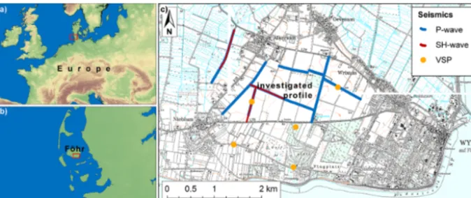
The test site is the North Sea island of Föhr (Fig. 1) that was investigated as a pilot area in the Interreg project CLIWAT (Harbo et al., 2011), which was co-financed by the European Union. The aim of CLIWAT was to analyse the influence of climate change to groundwater systems, and one major out-come was a hydrogeological model to forecast the ground-water evolution (Burschil et al., 2012a).
3.1 Geological evolution
The investigation area is located on the German North Sea island of Föhr, which is part of the UNESCO world her-itage Wadden Sea (Fig. 1). In general, the deeper subsurface was sedimented as part of the North German Basin while the landscape of Föhr was formed during the glacial and post glacial epoch (Scheer, 2012). The older sediments were de-posited under marine conditions since the Cretaceous age un-til the youngest Tertiary. For this reason, marine clay (mica clay) is found up to Miocene age. Sedimentation changed during the Pliocene, and sandy material (kaolin sand) was deposited until a climate change marked the beginning of the Pleistocene age. Glaciations from the Baltic–Scandinavian area reworked the shallow underground by alternating pro-cesses of glacial advance followed by erosion and sedimen-tation. In the region of Föhr, push moraines as well as a sys-tem of tunnel valleys were formed and refilled with glacial deposits (Scheer, 2012). The great outwash plains were in-creasingly flooded during the Holocene so that tidal mud de-posits were accumulated and formed large marshland areas. Finally, heavy floods in historical times eroded large parts and formed the present North Frisian Islands and Wadden Sea.
3.2 Geophysical and geological framework
In the project CLIWAT we accomplished a multidisciplinary geophysical acquisition (Burschil et al., 2012a). Between 2009 and 2011, we acquired seven seismic reflection profiles with P waves (in total 8 km) and three profiles with SH waves (in total 2.4 km). Five vertical seismic profiles (VSPs) were recorded with a 3C borehole geophone and the small electro-dynamical vibrator system ELVIS (Polom et al., 2011) with excitation in the vertical and horizontal–transversal direc-tions relative to the borehole location (Fig. 1). Maximum depths of five VSPs were in the range of 39–102 m, depend-ing on the borehole. Additionally, in 2008 the island was mapped within the airborne geophysics mapping project of LIAG (Leibniz Institute for Applied Geophysics; Wieder-hold et al., 2010) with the airborne electromagnetic system
SkyTEM (Sørensen and Auken, 2004). The result of the P-wave seismic survey was used as a priori information for the electromagnetic data inversion (Burschil et al., 2012b). The information transfer between the different geophysical methods improved the electric resistivity model of the island. Borehole logging data were evaluated statistically regard-ing electric resistivity as well as seismic velocity. This al-lowed for a petrophysical classification of sand, till, and clay (Burschil et al., 2012a). These lithological units form struc-tures such as push-moraines and buried valleys, which are consistent with the geological evolution of the region. A sim-plified hydrogeological model was compiled from all geo-physical and geological results for groundwater flow mod-elling (Burschil et al., 2012a).m
4 Seismic reflection field data 4.1 Seismic acquisition
Seismic equipment varied with surveys due to different wave types used for exploration. For two P-wave surveys we used the hydraulic vibrator systems of the LIAG, the MHV2.7 in 2009 and the new HVP-30 in 2010. As source signal we chose a linear sweep in the range of 30–240 Hz with 10 s duration. The source excited the seismic signal on a paved street in the western part of the profile and on grassland in the eastern part. The receivers were vertical geophones (20 Hz), planted in the green strip next to the line of the source locations (cross-line offset ca. 1 m). We chose a re-ceiver spacing of 2 m to enhance the near-surface resolution and fold. A combination of split-spread/roll along geometry was used (Fig. 2a) with a source spacing of twice the re-ceiver spacing (4 m). High-quality data had been acquired with this geometry before. We operated up to 268 active channels with Geometrics Geode seismographs with a max-imum in-line source–receiver offset of 360 m. This resulted in a fold between 47 and 72 in the main parts of the profiles. To avoid large data volumes, we recorded the seismic traces after vibro-seismic correlation with the Pelton Vib Pro input signal.
Figure 1. Overview maps with location of the island of Föhr (a, b). Detail map of the seismic locations on the island of Föhr (c). The profile
discussed in this paper is labelled.
profile. Here, the surface is paved, which helps avoiding the generation of surface waves.
All P-wave profiles show a good signal-to-noise ratio (Fig. 3). Seismic reflections can be detected down to 1 s two-way-travel time (TWT). In contrast, the shear waves of-fer a smaller signal-to-noise ratio (Fig. 4). Reflection hyper-bola signals are faint and within a reverberating background. Chevron patterns, also called herring-bone pattern, appear ir-regularly among shot gathers as part of the reverberations. The reflection signal bandwidth decreases with time. Below 0.7 s the signal vanishes, and further analysis in combination with seismic FD modelling is suggested.
4.2 Seismic processing
P-wave and shear-wave data processing differ due to different signal locations within the wave field. For the P-wave data, we set up a processing scheme (Table 1) focusing on the en-hancement of the reflections (e.g. Yilmaz, 2001). Processing was carried out with Landmark’s ProMAX 2D. The most im-portant processing steps turned out to be muting of the sur-face waves, spectral whitening, and dynamic corrections, in-cluding dip move-out corrections. The detailed velocity anal-ysis left a certain tolerance within the semblance calcula-tions. We therefore included geological a priori knowledge to reduce the uncertainty so that the resulting interval veloc-ity distribution better corresponds to the reflectors (Burschil et al., 2012a). At the end of the processing sequence, we ap-plied a time-migration to the CDP (common-depth-point)-stacked section. The migrated section was time-to-depth con-verted, using a single velocity function from one borehole, yielding a seismic depth section (Fig. 5).
To test the robustness of the result, a post-stack depth mi-gration of the non-migrated CDP-stacked section was also carried out (not shown here). It provided a similar seis-mic image as time-migration and time-to-depth conversion. Only small differences in the location of some reflectors of up to 3 m can be identified, but the reflector continuity remains. Therefore, we continued with the time-migrated, depth-converted section.
The shear-wave data contain surface wave interferences related to the specific shear-wave reflection move-out. This is the reason why we cannot simply mute the surface wave noise and purely focus on reflection signals, as we could for P waves. To enhance the reflection signals, we applied sev-eral techniques, e.g. fk filtering, spectral whitening, and de-convolution. Finally, automatic gain control (AGC, 300 ms) and fk-filtering with low-cutoff velocities below 350 m s−1 provided the best results (Table 1). This filter also removes a wide range of the chevron patterns that are present in the lower part of the seismograms around the shot location, de-picted in Fig. 4. In contrast to Polom (1997), who investi-gated a chevron pattern that originated in ghost sweeps, we cannot identify a comparable increase of the frequency with
time in the data. Here, the chevron pattern is rather monofre-quent and no ghost sweeps can be detected within the pattern. Velocity analysis was very difficult because reflections can only be identified sporadically and can hardly be traced through to neighbouring shots. This restrains velocity anal-ysis in CMP (common-mid-point)-sorted data. After nor-mal move-out correction and common midpoint stacking, we converted the section to depth with a velocity function de-rived from VSP measurements. The result is rather monofre-quent, but the till layer as well as deeper reflectors can be identified (Fig. 6). However, the quality of this shear-wave survey is less compared to the P-wave seismic results.
5 Synthetic data from finite-difference modelling To understand data quality differences between shear-wave measurements and compressional wave measurements on the island of Föhr, seismic wave-field modelling is introduced here for further data analysis. We chose the 2-D P/SV-version of SOFI for P-wave simulations and the 2-D SH version of SOFI for SH-wave modelling.
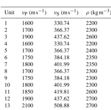
To create the input velocity and density models, we inter-preted the major structures of the P-wave seismic field data depth section (Fig. 5) and assigned P-wave velocities and densities according to geological and geophysical a priori in-formation (Fig. 7; Table 2). To supplement detailed shear-wave velocity information, we generated a cross-plot of ve-locity data (vPandvS) from the VSP surveys on the island of Föhr. This allowed us to calculate mean and median val-ues and the linear regression for different lithological classes. For statistical confidence, the number of classes was limited to those for which more than 20 velocity samples were avail-able. We then picked shear-wave velocities from the linear regression line of this cross-plot and thereby defined 14 litho-logical units with knownvPandvSvalues that constitute the input model (Fig. 8; Burschil et al., 2012a).
Figure 3. Seismic recordings of five single P-wave shots at different locations along the profile. The amplitude is displayed with an automatic
gain control (AGC) of 150 ms.
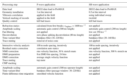
Table 1. Overview of processing of P-wave and SH-wave seismic field data including normal move-out (NMO) correction, dip move-out
(DMO) correction, and common midpoint (CMP) stacking (rms – root mean square).
Processing step P-wave application SH-wave application
Data load SEG2-data load to ProMAX SEG2-data load to ProMAX Geometry installation 1 m bin interval 0.5 m bin interval
Vibroseis correlation applied in the field using individual sweep Vertical stacking of records applied in the field twofold
Quality control kill bad traces kill bad traces
Refraction statics calculated from first breaks;vreplace=1600 m s−1 not applied
Amplitude scaling automatic gain control (300 ms length) automatic gain control (200 ms length) Fan filtering not applied low cut 350 m s−1
Deconvolution zero-phase spiking deconvolution (80 ms length) not applied
Time-variant filter bandpass filter (36–220 Hz) bandpass filter (30–160 Hz) Trace muting removal of noise cone not applied
Interactive velocity analysis 100 m node spacing, iteratively 100 m node spacing, iteratively Residual statics correction correlation auto statics not applied
NMO correction rms velocity function, 30 % stretch mute rms velocity function, 300 % stretch mute DMO preparation 8 m DMO bin spacing, 24 bins not applied
DMO correction average single velocity function not applied
Trace muting top mute not applied
CMP stacking
Amplitude scaling automatic gain control (300 ms operator length) not applied Time-variant filter bandpass filter (passage window: 30–220 Hz) not applied Finite-difference time migration smoothed velocity function not applied
Time-to-depth conversion single velocity function from VSP single velocity function from VSP
hosts the absorbing frame of 45 m. We did this to suppress surface multiples, which is the same approach that was used by Jones (2013). The effect of this absorbing frame is com-parable to a weathering layer with high parameter gradients. Additionally, we introduced a low-velocity layer with a free surface to test the simulation of a weathering layer. We used a zero-phase Ricker wavelet for the simulations instead of a vibro-seismic correlated sweep signal, i.e. a Klauder wavelet. This is a practical compromise which takes into account that the field data signals are absorbed to a certain degree and do
not show a white frequency spectrum. In contrast to the field data source signals, we used the same central frequency of the Ricker wavelet for P-wave simulation as well as for SH-wave simulation.
Figure 4. Seismic recordings of five single shear wave shots with
spatial divergence correction and AGC of 300 ms applied.
Table 2. Seismic velocities and densities for refined input model
(cf. Fig. 7b). Shear-wave velocity was calculated according to the cross-plot relation (Fig. 8).
Unit vP(m s−1) vS(m s−1) ρ(kg m−3)
1 1600 330.74 2200 2 1700 366.37 2300 3 1900 437.62 2600 4 1600 330.74 2200 5 1700 366.37 2400 6 1750 384.18 2350 7 1800 401.99 2350 8 1700 366.37 2300 9 1750 384.18 2300 10 1800 401.99 2300 11 1850 419.81 2600 12 1900 437.62 2700 13 2100 508.88 2700 14 2300 580.13 2700
5.1 Computational facility
The computer we are currently using for the simulations is a DELL Poweredge 910. It accommodates four CPUs Intel Xeon E7-4870 with 2.4 GHz, 10 cores each, DDR3 memory, and hyper threading. That results in 80 usable single CPUs with SuSE 11.4 Linux. Our computer hosts 512 GB of RAM, which is by far larger than needed for our 2-D models but will be necessary for larger 3-D simulations.
The computational time for modelling strongly depends on the number of modelled time steps and the size of the model. For P-wave modelling, we simulated the propaga-tion for 1 s and 20 000 time steps (Table 3). The computa-tional time for one single shot with the settings described was
ca. 30 min on 2 CPUs using the 2-D P–SV version of SOFI. 2-D shear-wave modelling with the SH version of SOFI was much faster per computational step. Simulating 2.5 s, i.e. 50 000 time steps, of wave propagation took ca. 60 min per shot.
5.2 P-wave modelling
In the simulated single shot data (Fig. 10), we detect direct P and SV waves as well as reflections of P and SV waves. The surface wave pattern of the field data is not present in the synthetic data, (cf. noise cone in Fig. 3). P-wave reflections can be tracked in the synthetic data, even in those regions where they are usually covered by surface waves. Also, the simulated data have an apparent higher frequency content, not showing the typical subsurface low-pass filter effect.
We applied a simple processing scheme to all 300 mod-elled single shots comprising amplitude control, frequency filtering, normal move-out correction, common midpoint stacking, time-migration, and time-to-depth conversion. Stacking velocities were picked via an interactive velocity analysis from CMP gathers.
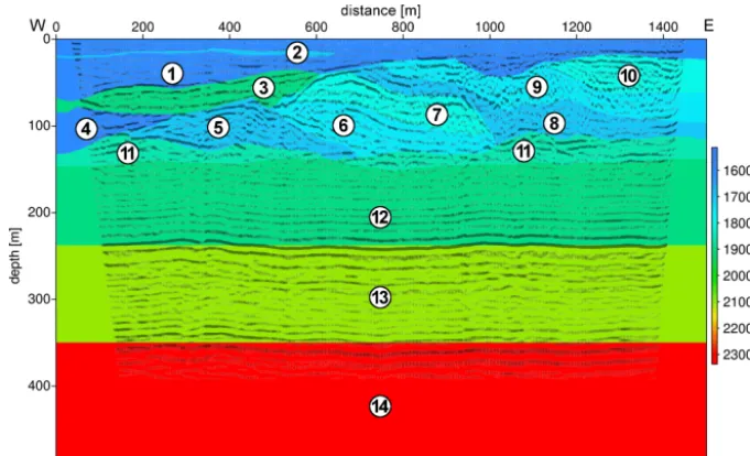
In the migrated depth section (Fig. 11a), the uppermost reflector at 30 m is faint. Below, two strong reflectors mark the upper and lower boundaries of the till unit. The upper re-flector can be traced through the entire section with varying amplitude. Also, a large number of reflectors with different amplitudes is imaged. In the central part of the seismogram at 150 m depth, two close reflectors mark the lower end of the complex geological units. Below, two nearly horizontal re-flectors at 250 and 380 m depths are present. At the western and eastern edges of the section the migration process gener-ated minor artefacts. Because this P-wave depth section was basically able to explain the P-wave field data, we continued with the simulation of the shear-wave field data instead of a further study of additional features present in the P-wave field data, like surface-wave ground roll.
5.3 Shear-wave modelling
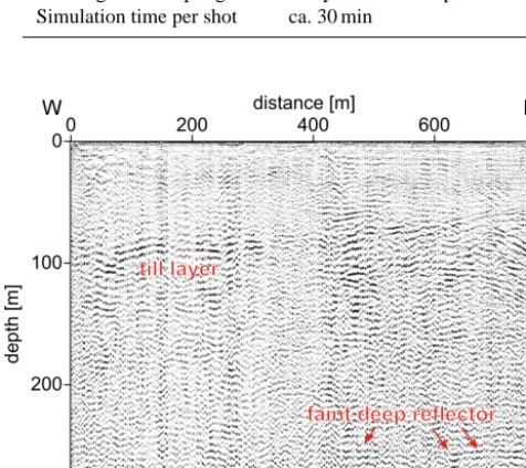
Figure 5. Final time migrated depth section of the P-wave seismic survey with AGC of 200 ms applied before time-to-depth conversion. The
blue box marks the position of the SH-wave section (Fig. 6).
Table 3. Input parameters for FD modelling. Grid size is specified by node spacing dh, and absorbing frame width FW characterizes the
width of the absorbing frame. dt specifies the calculated time stepping.
P wave SH wave
Model size 1200×1100 nodes, dh = 0.5 m 1200×1100 nodes, dh = 0.5 m Propagation time time = 1 s, time steps dt = 5×10⁻⁵s time = 2.5 s, time steps dt = 5×10⁻⁵s
Source wavelet Ricker, 100 Hz central frequency, vertical force Ricker, 100 Hz central frequency, SH-wave force Boundary FW = 90 nodes, 6 % damping per node FW = 90 nodes, 6 % damping per node
Receiver vertical geophone, spacing = 2 nodes horizontal (SH) geophone, spacing = 2 nodes Seismograms sampling rate every 10th time step every 20th time step
Simulation time per shot ca. 30 min ca. 60 min
Figure 6. Depth-converted stack of the shear-wave seismic survey
with AGC of 300 m applied after time-to-depth conversion.
6 Discussion
Figure 7. Input model of P-wave velocity. The P-wave field depth section is superimposed. Numbers 1–14 mark the units listed in Table 2.
Figure 8.vP/vScross-plot from VSP data colour-coded for
differ-ent lithologies. Additionally, median values, mean values and the linear regression (LinReg) are indicated. The shear-wave velocity was calculated for each P-wave velocity with the relation resulting from the linear regression.
and land streamer is the favourite choice for shear-wave seis-mics. General data processing reported in some of the stud-ies is similar to the processing we finally applied (Table 1). Sauvin et al. (2014) reported the application of elevation stat-ics for only one of their shear-wave profiles. None of the authors reported refraction statics for shear waves. In some cases, differences in shear-wave processing are related to de-convolution and spectral whitening, which was applied by Pugin et al. (2009b) and Sauvin et al. (2014). Here, deconvo-lution and spectral whitening did not provide success.
Figure 9. Westernmost model segment of the input model.
Indi-vidual single shots were modelled and the yellow stars mark the locations of the shot points (every 4 m). Black triangles mark the receiver position (each 1 m). The region of the absorbing frame is faded out.
Figure 10. Five different synthetic P-wave single shots. Shot gathers are displayed with 150 ms AGC.
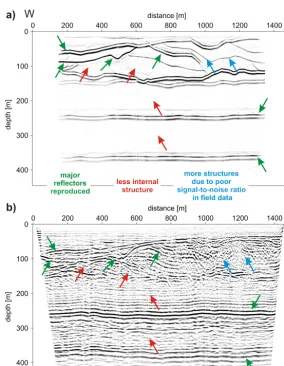
Figure 11. FD modelling of the P-wave section (a) and section from field data (b). Both sections are displayed with AGC of 100 ms.
waves are not present in VSP data and do not affect data qual-ity significantly. Scattering also affects the surface data more
Figure 12. Five different shear wave FD-modelling single shots.
Shot gathers with 120 m spread, amplified by 300 ms AGC, are dis-played.
longer for surface data than for VSP data. If this explanation is true, we will have to take small-scale inhomogeneities and a weathering layer as origin of surface waves into account for future studies.
6.1 Influence on data quality in land seismic surveys In general, a number of factors can influence the quality of land seismics data, listed and illustrated in Sheriff (1975). Typical factors, one would assume to be the most likely in our case, are source strength, inappropriate coupling of sources and receivers, superimposed surface waves, multiples, scat-tering, and intrinsic absorption (Q).
The vertical hydraulic vibrator sources MHV2.7 and HVP-30 have proven their ability to reach reflectors at least 2 km deep (Buness et al., 2009). The LIAG shear-wave vibra-tor source MHV-4S has been able to generate clear reflec-tions at least as deep as 200 m in fluviatile and marine deposits (Polom et al., 2010). Sauvin et al. (2014) used a wheelbarrow-mounted microvibrator source for the anal-ysis of quick clays. Their data show clear reflections from 40 m below ground level within fluviatile and marine sedi-ments. In the underlying bedrock, reflections can be traced down to 120 m depth. Malehmir et al. (2013) report clear reflections in a similar environment from at least 40 m be-low ground level with the same source. This means that even small sources are able to create reflections from at least 40 m below the source. Pugin et al. (2009b) used an IVI Minivib on a minibuggy carrier, which is comparable to the MHV-4S. They show SH-wave reflections down to about 50 m in glacial deposits before reaching the bedrock. In the light of these studies, the MHV-4S source can be expected to be strong enough to image the glacially overworked deposits
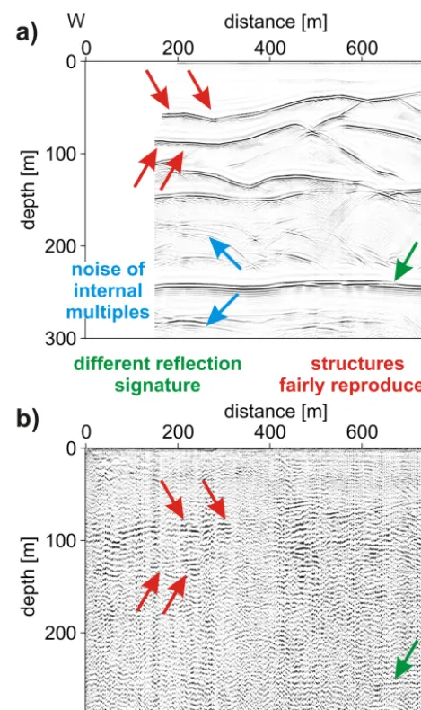
Figure 13. Shear wave FD-modelling section (a) and section from
field data (b). Both sections are displayed with AGC of 300 ms ap-plied.
down to 150 m. In fact, the SH-wave image shows faint re-flections even from ca. 270 m depth (Fig. 6).
which geophones are directly fixed to aluminium plates that have a gravitational three-point contact to the ground. This system has proven to receive good shear-wave signals from the subsurface before (Polom et al., 2010; Krawczyk et al., 2013; Malehmir et al., 2013). On one SH-wave profile on gravel, Sauvin et al. (2014) used the same streamer but on grassland they planted the geophones in the ground. They do not report any difference in data quality. Pugin et al. (2004, 2009a, b) use a different land streamer system that works suc-cessfully as well. In the field, we took care that the geophone coupling was good. Every time a new streamer position was reached, a noise test was carried out and noisy geophones were coupled to the ground by hand. We therefore expect coupling to be sufficient.
Surface waves are an important degradation factor for shear-wave reflection surveys. Here, the reflection hyperbola often interferes with surface wave (Love wave) signals; cf. surface waves (Fig. 3) and reflection hyperbolas (Fig. 4). This factor has complicated the application of shear waves in the past and still limits the application of this method. However, the observation that a high-velocity layer at the surface sup-presses the generation of surface waves in shear-wave explo-ration (e.g. Inazaki, 2004) was an important step to overcome this limitation in many urban applications and even in ru-ral environments if paved or consolidated roads are present. Even though surface waves are often excited during an SH-wave surveys on unconsolidated surfaces, SH-SH-wave reflec-tion seismics surveys have been successful in these condi-tions (e.g. Malehmir et al., 2013; Sauvin et al., 2014). Polom et al. (2013) identify partly dispersive Love waves that show a similar signature as the chevron pattern depicted in Fig. 4. In their case and in our case, these waves seem to be linked to the shot-point location. Even neighbouring shot points show strong variations in this respect. For instance, in Fig. 4 we show shot gathers with shot-point locations of FFID’s 1126 and 1127 that are just 4 m apart. To cancel surface waves with a linear move out or mild dispersive character fk filtering is often successfully used (e.g. Polom et al., 2013; Sauvin et al., 2014). We successfully applied an fk filter as well (Table 1), but this did not improve the coherency of reflectors in the final depth section (Fig. 6).
Further issues for data quality of land seismics data are intrinsic damping (e.g. Kang and McMechan, 1994) and
6.2.1 P-wave shot gathers
The simulated P-wave and the corresponding field data of single shot seismograms (Figs. 3, 10) contain reflection events that show a similar basic waveform. However, the field data (Fig. 3) are much noisier, in particular before the first break as well as inside the surface-wave cone. No reflections are detectable inside this field data cone whereas in the syn-thetic data (Fig. 10) reflections can be traced through all parts of the seismogram. This can be explained to a large degree by the lack of a weathering layer in the models. The absence of this layer prevents the build-up of simulated surface waves and thus, a surface wave cone is missing in simulated shot records. Therefore, the refracted wave in the field data corre-sponds to the direct wave in the synthetic data.
Another noticeable observation is the signature of the re-flections. In general, the reflection signals of the synthetic data seem to be more focused whereas many of the reflec-tions within the field data seem to be made up of a number of oscillations/reverberations instead of single reflections (com-pare reflection signal at 0.3 s in Figs. 3 and 10). We expect an additional fine-layering within the 14 units of the input model to be able to reproduce this observation (Fig. 10). Per-haps, the simulation of a multilayer surface unit, related to the weathering zone might also help explaining the rever-beration observation. We also simulated a low-velocity top layer (thickness = 10 m,vP=500 m s−1,vS=200 m s−1, and
6.2.2 SH-wave shot gathers
Shear-wave shot simulations show larger differences com-pared with their corresponding field data (Figs. 4 and 12). The clear and continuous reflections in the synthetic data are not present in the field data. Some of the field records show the mentioned chevron pattern parallel to the first break with varying amplitude (Fig. 4) that does not show up in the syn-thetic data. In the model, we did not consider very shallow structures that could create Love waves.
The spectrum of the synthetic data does not change with time in the seismogram (Fig. 12). The Ricker wavelet has the same spectral shape for shallow reflections as for deep re-flections. This is no surprise since up to this point we have not included any kind of signal damping in the model like in-trinsic damping or sources for attenuation through scattering or interference. In contrast, the field data signals for longer travel times lose some of the higher-frequency components (Fig. 4). This indicates some kind of intrinsic or scattering attenuation. However, this cannot explain the lateral appear-ance variation among shot gathers of the shear-wave data.
6.2.3 P-wave depth section
The post-stack time-migrated P-wave depth section of syn-thetic data shows less noise and less amplitude variability while the corresponding field data show natural levels of dif-ferent signals and thus contain more information about small-scale and internal structures (Fig. 11). The modelled depth section reproduces the major features of the field data. The till top reflector between 50 and 80 m depth appears con-tinuous and two deep reflectors show as well. Some of the dipping reflectors in this modelled section add details that similarly appear in the field data.
The field data section (Fig. 11b) can be divided into two parts: excitation on paved street and on grassland. Within the seismic field data section, we detected a lack of resolution in the grassland part (about 900–1400 m, marked with blue arrows in Fig. 11b) that is not present in the modelled data. However, we have not implemented the structural complex-ity of unconsolidated grassland as a near-surface weathering layer, i.e. large velocity contrasts, inhomogeneities, and in-trinsic damping, in the model so far.
In general, the reflection signatures in the field data spa-tially vary more strongly than in the synthetic data (Fig. 11). Sources for these observations in the field data can be intrin-sic damping, scattering attenuation including fine layering, and inhomogeneous lithological units. All of these features were not included in the input model (Fig. 7). In a natural en-vironment, complex structures or fine layers can be sources of multiples and wave conversion that subsequently can pose similar challenges to data processing like random noise sig-nals do. Since the model consisted of comparatively large units, this kind of noise was not simulated.
6.2.4 SH-wave stacked sections
The SH-wave stacked sections of synthetic data and field data (Fig. 13) differ more than the P-wave sections. While no clear interpretation can be carried out for the stacked field data, the stacked section from the modelled data set well repro-duces the input model. For example reflector segments occur at 90 m depth, which correspond to the interface of the sub-horizontal layer at 90 m (top till layer) and at 250 m depth corresponding to the first deep reflector in the P-wave seis-mic section. Nonetheless, the reflection signatures in the field data are much noisier than in the synthetic data.
7 Summary and outlook
Shear-wave field data recorded on the island of Föhr showed less quality compared with their compressional wave coun-terparts. To comprehend the reasons for this quality differ-ence, we used seismic wave-field modelling within simple models of the subsurface, using the seismic field geometry. We chose finite-difference modelling to try to reproduce the field data because of its ability to simulate the entire wave field and to allow for arbitrary input models. We come to the following conclusions.
1. We were able to simulate P waves that show clear first-order similarities compared with the P-wave field data. 2. Simplified FD modelling does not explain the small
signal-to-noise ratio of the shear-wave field data. For future analyses, we therefore suggest to consider addi-tional complexity in the subsurface model that will presum-ably be able to explain the different quality of compressional and shear-wave field data. The most important additional fac-tors are intrinsic damping, thin layers within the modelled units, a complex near-surface weathering layer structure, and heterogeneous material within the layers. While 2-D calcula-tions gain faster results and allow testing the effect of differ-ent features, the full complexity of field acquisition may be understood using 3-D simulations in the future.
Acknowledgements. We acknowledge Karlsruhe Institute of Technology (KIT) for providing an academic licence of the SOFI software package. We thank Y. Yang (referee), the anonymous second referee, and Helga Wiederhold for their helpful comments.
Science Journal, 57, 338–366, 2009.
Burschil, T., Scheer, W., Kirsch, R., and Wiederhold, H.: Compil-ing geophysical and geological information into a 3-D model of the glacially-affected island of Föhr, Hydrol. Earth Syst. Sci., 16, 3485–3498, doi:10.5194/hess-16-3485-2012, 2012a.
Burschil, T., Wiederhold, H., and Auken, E.: Seismic re-sults as a-priori knowledge for airborne TEM data inver-sion – A case study, J. Appl. Geophys., 80, 121–128, doi:10.1016/j.jappgeo.2012.02.003, 2012b.
Carcione, J. M., Herman, G. C., and ten Kroode, A.: Seismic mod-eling, Geophysics, 67, 1304–1325, 2002.
Cheraghi, S., Malehmir, A., Bellefleur, G., Bongajum, E., and Bas-tani, M.: Scaling behavior and the effects of heterogeneity on shallow seismic imaging of mineral deposits: A case study from Brunswick No. 6 mining area, Canada, Journal of Applied Geo-physics, 90, 1–18, 2013.
Fichtner, A., Bleibinhaus, F., and Capdeville, Y.: Full seismic wave-form modelling and inversion, Springer, 2011.
Gold, N., Shapiro, S. A., and Burr, E.: Modeling of high contrasts in elastic media using a modified finite difference scheme, in: 68th Annual International Meeting, Soc. Explor. Geophys., Expanded Abstracts, 1997.
Groos, L., Schäfer, M., Forbriger, T., and Bohlen, T.: On the sig-nificance of viscoelasticity in a 2D full waveform inversion of shallow seismic surface waves, in: 74th EAGE Conference & Ex-hibition, Copenhagen, 2012.
Harbo, M. S., Pedersen, J., Johnsen, R., and Peteren, K.: Groundwa-ter in a Future Climate: The CLIWAT Handbook, The CLIWAT Project Group, 2011.
Hardage, B. A., DeAngelo, M. V., Murray, P. E., and Sava, D.: Mul-ticomponent seismic technology, Society of Exploration Geo-physicists, 2011.
Inazaki, T.: High-resolution seismic reflection surveying at paved areas using an S-wave type land streamer, Explor. Geophys., 35, 1–6, 2004.
Jones, I. F.: Tutorial: the seismic response to strong vertical ve-locity change, First Break, 31 (6), 79–90, doi:10.3997/1365-2397.2013018, 2013.
Jørgensen, F., Scheer, W., Thomsen, S., Sonnenborg, T. O., Hinsby, K., Wiederhold, H., Schamper, C., Burschil, T., Roth, B., Kirsch, R., and Auken, E.: Transboundary geophysical mapping of geo-logical elements and salinity distribution critical for the assess-ment of future sea water intrusion in response to sea level rise, Hydrol. Earth Syst. Sci., 16, 1845–1862, doi:10.5194/hess-16-1845-2012, 2012.
N., Polom, U., and Persson, L.: Geophysical assessment and geotechnical investigation of quick-clay landslides – a Swedish case study, Near Surf. Geophys., 11, 341–350, 2013.
Miller, R. D.: Introduction to this special section: Urban geophysics, The Leading Edge, 32, 248–249, 2013.
Plessix, R.-E.: Waveform inversion overview: Where are we? And what are the challenges?, in: 74th EAGE Conference & Exhibi-tion, Copenhagen, 2012.
Polom, U.: Elimination of source-generated noise from correlated vibroseis data (the “ghost-sweep” problem), Geophys. Prospect., 45, 571–591, 1997.
Polom, U., Hansen, L., Sauvin, G., L’Heureux, J.-S., Lecomte, I., Krawczyk, C. M., Vanneste, M., and Longva, O.: High-resolution SH-wave seismic reflection for characterization of on-shore ground conditions in the Trondheim harbor, central Nor-way, in: Advances in Near-Surface Seismology and Ground-Penetrating Radar, SEG, Tulsa, 297–312, 2010.
Polom, U., Druivenga, G., Grossmann, E., Grüneberg, S., and Rode, W.: Transportabler Scherwellenvibrator, Patent application, Ger-man Patent and Trade Mark Office, 5 pages, 2011 (in GerGer-man). Polom, U., Bagge, M., Wadas, S., Winsemann, J., Brandes, C.,
Binot, F., and Krawczyk, C.: Surveying near-surface depocen-tres by means of shear wave seismics, First Break, 31 (8), 67–79, 2013.
Pugin, A. J. M., Larson, T. H., Sargent, S. L., McBride, J. H., and Bexfield, C. E.: Near-surface mapping using SH-wave and P-wave seismic land-streamer data acquisition in Illinois, US, The Leading Edge, 23, 677–682, 2004.
Pugin, A. J.-M., Pullan, S. E., and Hunter, J. A.: Multicomponent high-resolution seismic reflection profiling, The Leading Edge, 28, 1248–1261, 2009a.
Pugin, A. J.-M., Pullan, S. E., Hunter, J. A., and Oldenborger, G. A.: Hydrogeological prospecting using P-and S-wave landstreamer seismic reflection methods, Near Surf. Geophys., 7, 315–327, 2009b.
Robertsson, J. O., Blanch, J. O., and Symes, W. W.: Viscoelastic finite-difference modeling, Geophysics, 59, 1444–1456, 1994. Robertsson, J. O., Bednar, B., Blanch, J., Kostov, C., and van
Ma-nen, D.-J.: Introduction to the supplement on seismic modeling with applications to acquisition, processing, and interpretation, Geophysics, 72, SM1–SM4, 2007.
Rumpel, H.-M., Binot, F., Gabriel, G., Siemon, B., Steuer, A., and Wiederhold, H.: The benefit of geophysical data for hydrogeo-logical 3D modelling an example using the Cuxhaven buried val-ley, Z. Dtsch. Ges. Geowiss., 160, 259–269, 2009.
Saenger, E. H., Gold, N., and Shapiro, S. A.: Modeling the prop-agation of elastic waves using a modified finite-difference grid, Wave Motion, 31, 77–92, 2000.
Sauvin, G., Lecomte, I., Bazin, S., Hansen, L., Vanneste, M., and L’Heureux, J.-S.: On the integrated use of geophysics for quick-clay mapping: The Hvittingfoss case study, Norway, J. Appl. Geophys., 106, 1–13, doi:10.1016/j.jappgeo.2014.04.001, 2014. Scheer, W.: Geologie und Landschaftsentwicklung von Schleswig-Holstein, in: Der Untergrund von Föhr: Geologie, Grundwasser und Erdwärme; Ergebnisse des Interreg-Projektes CLIWAT, 11– 20, Schriftenreihe LLUR SH – Geologie und Boden, Landesamt für Landwirtschaft, Umwelt und ländliche Räume des Landes Schleswig-Holstein, Flintbek, 2012 (in German).
Sheriff, R. E.: Factors affecting seismic amplitudes, Geophys. Prospect., 23, 125–138, 1975.
Sheriff, R. E. and Geldart, L. P.: Exploration Seismology, Cam-bridge University Press, 1995.
Sørensen, K. I. and Auken, E.: SkyTEM – a new high-resolution helicopter transient electromagnetic system, Explor. Geophys., 35, 194–202, 2004.
Steeples, D. W. and Miller, R. D.: Seismic reflection methods ap-plied to engineering, environmental, and groundwater problems, Geotechnical and Environmental Geophysics, 1, 1–30, 1990. Virieux, J.: P-SV wave propagation in heterogeneous media:
Velocity-stress finite-difference method, Geophysics, 51, 889– 901, 1986.
Virieux, J. and Operto, S.: An overview of full-waveform inversion in exploration geophysics, Geophysics, 74, WCC1–WCC26, 2009.
Wiederhold, H., Siemon, B., Steuer, A., Schaumann, G., Meyer, U., Binot, F., and Kühne, K.: Coastal aquifers and saltwater intru-sions in focus of airborne electromagnetic surveys in Northern Germany, in: Proc. 21st Salt Water Intrusion Meeting, Azores, 94–97, 2010.