www.the-cryosphere.net/10/2027/2016/ doi:10.5194/tc-10-2027-2016
© Author(s) 2016. CC Attribution 3.0 License.
Sea-ice indicators of polar bear habitat
Harry L. Stern1and Kristin L. Laidre1,2
1Polar Science Center, Applied Physics Laboratory, University of Washington, 1013 NE 40th Street, Seattle, WA 98105, USA
2Greenland Institute of Natural Resources, Box 570, 3900 Nuuk, Greenland
Correspondence to:Harry L. Stern (harry@apl.washington.edu)
Received: 5 May 2016 – Published in The Cryosphere Discuss.: 24 May 2016
Revised: 18 August 2016 – Accepted: 24 August 2016 – Published: 14 September 2016
Abstract. Nineteen subpopulations of polar bears (Ursus maritimus) are found throughout the circumpolar Arctic, and in all regions they depend on sea ice as a platform for travel-ing, hunttravel-ing, and breeding. Therefore polar bear phenology – the cycle of biological events – is linked to the timing of sea-ice retreat in spring and advance in fall. We analyzed the dates of sea-ice retreat and advance in all 19 polar bear sub-population regions from 1979 to 2014, using daily sea-ice concentration data from satellite passive microwave instru-ments. We define the dates of sea-ice retreat and advance in a region as the dates when the area of sea ice drops below a certain threshold (retreat) on its way to the summer mini-mum or rises above the threshold (advance) on its way to the winter maximum. The threshold is chosen to be halfway be-tween the historical (1979–2014) mean September and mean March sea-ice areas. In all 19 regions there is a trend to-ward earlier sea-ice retreat and later sea-ice advance. Trends generally range from−3 to−9 days decade−1in spring and from +3 to+9 days decade−1 in fall, with larger trends in the Barents Sea and central Arctic Basin. The trends are not sensitive to the threshold. We also calculated the number of days per year that the sea-ice area exceeded the threshold (termed ice-covered days) and the average sea-ice concen-tration from 1 June through 31 October. The number of ice-covered days is declining in all regions at the rate of−7 to −19 days decade−1, with larger trends in the Barents Sea and central Arctic Basin. The June–October sea-ice concentra-tion is declining in all regions at rates ranging from −1 to −9 percent decade−1. These sea-ice metrics (or indicators of habitat change) were designed to be useful for management agencies and for comparative purposes among subpopula-tions. We recommend that the National Climate Assessment
include the timing of sea-ice retreat and advance in future reports.
1 Introduction
Table 1. Polar bear subpopulation region names, abbreviations, and areas. See Fig. 1 for a map of the regions. The area of each region includes the marine portion only, not land. The number of cells is the number of SSM/I grid cells. The percent of total area is with respect to all regions (last row). The percent of area shallower than 300 m and deeper than 300 m are given in the last two columns. The pole hole (second to last row) is the circular area around the North Pole excluded from analysis due to the satellite orbits. The Arctic Basin region (AB) surrounds the pole hole but does not include it. All regions includes all 19 subpopulation regions plus the pole hole.
Abbreviation Subpopulation Number of Area % of total % %
cells (103km2) area ≤300 m > 300 m
KB Kane Basin 81 53 0.3 68 32
BB Baffin Bay 1042 656 4.3 28 72
LS Lancaster Sound 380 243 1.6 73 27
NW Norwegian Bay 108 70 0.5 84 16
VM Viscount Melville 157 101 0.7 64 36
NB Northern Beaufort 1055 677 4.4 23 77
SB Southern Beaufort 529 333 2.2 59 41
MC M’Clintock Channel 224 140 0.9 100 0
GB Gulf of Boothia 100 62 0.4 99 1
FB Foxe Basin 883 528 3.4 97 3
WH Western Hudson Bay 326 188 1.2 100 0
SH Southern Hudson Bay 744 417 2.7 100 0
DS Davis Strait 2416 1367 8.9 40 60
EG East Greenland 2237 1387 9.0 27 73
BS Barents Sea 2379 1540 10.0 63 37
KS Kara Sea 1645 1054 6.9 87 13
LP Laptev Sea 2169 1393 9.1 84 16
CS Chukchi Sea 1840 1117 7.3 98 2
AB Arctic Basin 4307 2813 18.3 15 85
Pole hole 1799 1193 7.8 0 100
All regions 24 421 15 332 100.0 50 50
2014; Laidre et al., 2015a; Obbard et al., 2016), or the sea-ice concentration (Rode et al., 2012; Peacock et al., 2012, 2013). Sea-ice metrics have mainly been selected based on the specific region under study or developed for single stud-ies or data sets. There is a need to develop standardized cir-cumpolar metrics of polar bear habitat based on the satellite record of sea ice that allow for regional comparisons of habi-tat change and for tracking changes into the future, e.g., as in Vongraven et al. (2012). Thus the objective of this study is to propose and produce metrics of polar bear sea-ice habitat that are also relevant to other Arctic marine mammal (AMM) species.
In this study we used daily sea-ice concentration data to calculate several sea-ice metrics for each of the 19 polar bear subpopulation regions for the period 1979–2014. The metrics are date of spring sea-ice retreat, date of fall sea-ice advance, average sea-ice concentration from 1 June to 31 October, and the number of ice-covered days per year. We calculated each metric for the total marine area of each region and for the shallow depths only (≤300 m). Shallow depths are more bi-ologically productive and are considered to be better polar bear habitat (Durner et al., 2009).
Several previous studies have divided the Arctic into dis-tinct regions and calculated the sea-ice area trend in each region (e.g., Stroeve et al., 2012; Perovich and
Richter-Menge, 2009; Parkinson and Cavalieri, 2008). While this is a straightforward and useful way to document changes in sea ice, other metrics of sea-ice habitat are more relevant to ma-rine mammals whose life history events, such as hunting and breeding, depend on the annual retreat of sea ice in the spring and advance in the fall. Many ecologically important regions of the Arctic are ice covered in winter and ice free in summer and will probably remain so for a long time into the future. Therefore the dates of sea-ice retreat in spring and advance in fall, and the interval of time between them, are key indi-cators of climate change for ice-dependent marine mammals (Stirling et al., 1999; Stirling and Parkinson, 2006).
2 Data
algo-Table 2.Recent literature where sea-ice metrics were used for analysis of polar bear habitat. Note that these studies examined habitat for a single polar bear subpopulation (or geographically close set of subpopulations). Bold text gives names of sea-ice metrics. Abbreviations: PM (passive microwave), SIC (sea-ice concentration), CIS (Canadian Ice Service).
Subpopulation Data Years Methods for sea-ice metric Reference
Western Hudson Bay
Daily PM SIC
1979–2004 Calculated daily percent sea-ice cover in the re-gion. Date of spring sea-ice breakup is the date when the ice cover fell below 50 %.
Stirling and Parkinson (2006)
Western Hudson Bay
Daily PM SIC
1984–2004 Date of spring sea-ice breakup is the date when the ice cover fell below 50 %
(same as Stirling and Parkinson, 2006).
Regehr et al. (2007)
Southern Hudson Bay
Daily PM SIC
1984–2003 Date of spring sea-ice breakup is the date when the ice cover fell below 50 % (same as Stirling and Parkinson, 2006).
Date of fall sea-ice freeze-upis the date when the ice cover rose above 50 %.
Ice-free periodis the number of days between breakup and freeze-up.
Obbard et al. (2007)
Southern Beaufort Sea
Daily PM SIC
2001–2005 Calculated the daily percent sea-ice cover for the continental shelf only (depth < 300 m). Number of ice-free daysis the number of days per calendar year with ice cover < 50 %.
Regehr et al. (2010)
Northern Beaufort Sea
Daily PM SIC
1979–2006 Mean annual number of grid cells with sea-ice concentration>50%, calculated for conti-nental shelf only (depth < 300 m) and excluding a buffer of one ocean grid cell along all coast-lines. Second sea-ice covariate is derived from theresource selection functionsof Durner et al. (2009).
Stirling et al. (2011)
Baffin Bay, Davis Strait
Mean weekly SIC (CIS)
1977–2010 Mean weekly sea-ice concentrationfrom 15 May to 15 October.
Rode et al. (2012)
Chukchi Sea, South-ern Beaufort Sea
Daily PM SIC
1985–1993, 2007–2010
Reduced-ice days per yearis the number of days with sea-ice area < 6250 km2(continental shelf of each region only, depth < 300 m). Distance to ice edgeis the daily minimum dis-tance from continental shelf to pack ice, aver-aged over all days in September. When pack ice is over the continental shelf the distance is set to zero.
Rode et al. (2014)
Baffin Bay Daily PM SIC
1979–2009 Sea-ice concentration in April, May, and June for the continental shelf only (depth < 300 m). (Note that the continental shelf consists of two parts: Baffin Island in the west and Greenland in the east.)
Peacock et al. (2012)
Davis Strait Mean weekly SIC (CIS)
1974–2007 Mean weekly sea-ice concentrationfrom 14 May to 15 October.
Table 2.Continued.
Subpopulation Data Years Methods for sea-ice metric Reference
Canadian Arctic Archipelago
MIT general circulation model (GCM)
2006–2100 Future projections of sea ice were made using the MIT GCM with 18 km grid size and monthly output, forced by “business as usual” RCP8.5 emission sce-nario.
Month of spring sea-ice breakupis the first month in a given year with sea-ice concentration < 50 %. Month of fall sea-ice freeze-upis the first month af-ter breakup with sea-ice concentration≥10 %. Ice-free seasonis the time from breakup to freeze-up. If all months of the year have sea-ice concentra-tion < 10 % then the ice-free season is 12 months.
Hamilton et al. (2014)
Western Hudson Bay
Daily PM SIC
1979–2012 Calculated daily percent sea-ice cover in the region. Date of spring sea-ice breakup is the date when the ice cover fell below 50 % (same as Stirling and Parkinson, 2006) and stayed below 50 % for at least 3 consecutive days.
Date of fall sea-ice freeze-upis the date when the ice cover rose above 50 % and stayed above 50 % for at least 3 consecutive days.
Ice decayis the rate of sea-ice loss from 1 May until the date of complete disappearance of sea ice, calcu-lated as the absolute value of the slope of the ordinary least squares regression line of ice concentration vs. time.
Lunn et al. (2014)
East Green-land
Daily PM SIC
1979–2012 Calculated the daily sea-ice area in the region. De-fined threshold area A as halfway between mean March ice area and mean September ice area, where the means are calculated over the baseline period 1979–1988.
Date of spring sea-ice breakupis the date when ice area fell below threshold area A.
Date of fall sea-ice freeze-up is the date when ice area rose above threshold area A.
Laidre et al. (2015a)
Chukchi Sea, South-ern Beaufort Sea
Daily PM SIC
1979–2013 Calculated the daily sea-ice area in each region. De-fined threshold area A as halfway between mean March ice area and zero area, where the mean March area is calculated over the baseline period 1979– 2013.
Ice-covered days is the number of days each year with ice area > threshold area A.
Calculated the mean number of ice-covered days for 1994–2013 and then projected the number of ice-covered days forward in time.
Regehr et al. (2015)
Southern Beaufort Sea
2001–2010 Summer habitat is the sum of monthly indices of the area of optimal polar bear habitat over the conti-nental shelf for July through October each year (from Durner et al., 2009).
Melt season is the time between melt onset and freeze onset (“inner melt length” from Stroeve et al., 2014).
Bromaghin et al. (2015)
Southern Hudson Bay
Daily PM SIC
1980–2012 Date of spring sea-ice breakup is the date when mean ice concentration falls below 5 %.
Date of fall sea-ice freeze-upis the date when mean ice concentration rises above 5 %.
Figure 1.Map of the 19 PBSG polar bear subpopulation regions, with shallow depths (≤300 m) in blue. See Table 1 for subpopula-tion names corresponding to the abbreviasubpopula-tions on the map.
rithm, and are provided in a polar stereographic projection (true at 70◦N) with a nominal grid cell size of 25×25 km (cell size varies slightly with latitude). Temporal coverage is every other day from 26 October 1978 through 9 July 1987, then daily through 31 December 2014.
Concerning the accuracy of the sea-ice concentration data, the product documentation states that it is within ±5 % of the actual sea-ice concentration in winter and±15 % in sum-mer when melt ponds are present on the sea ice and that the accuracy is best for thick ice (> 20 cm) and high ice concen-tration (NSIDC, 2015). This means that accuracy is less in the marginal ice zone – the band of low ice concentration between open water and consolidated pack ice. Ivanova et al. (2015) found that all passive microwave sea-ice retrieval algorithms underestimated sea-ice concentration in the pres-ence of melt ponds and thin ice. Thus our estimates of daily sea-ice area in each region are undoubtedly biased low, but a consistent bias over time would not affect trends computed from the data.
The spatial coverage of the sea-ice concentration data ex-cludes a small circle around the North Pole, due to the satel-lite orbits. This “pole hole” is entirely surrounded by the Arc-tic Basin region (AB in Fig. 1 and Table 1). Although the size of the pole hole became smaller in 1987 with the advent of a new satellite and instrument, we use the larger pre-1987 pole hole for consistency of calculations throughout the pe-riod 1979–2014. Our Arctic Basin region does not include the pole hole; it surrounds the pole hole.
To identify shallow depths (≤300 m) we used bathymetry from ETOPO1, a 1 arcmin global relief model of Earth’s sur-face that integrates land topography and ocean bathymetry, built from numerous global and regional data sets (Amante and Eakins, 2009). We averaged the ETOPO1 data over each SSM/I grid cell to obtain the mean ocean depth for each cell, which we then used to distinguish the continental shelf (≤300 m depth) from the deeper ocean. Table 1 gives the ma-rine area of the 19 subpopulation regions, as well as the per-cent of the area shallower than 300 m and deeper than 300 m.
3 Methods
3.1 Preliminary data processing
Sea-ice area is defined assea-ice concentration×grid cell areasummed over cells with sea-ice concentration greater than 15 %. For each region, we calculated the daily (or every-other-day prior to 1987) sea-ice area over two sets of grid cells: (1) all cells in the region and (2) those cells in which the mean ocean depth is≤300 m. We note that the 15 % thresh-old is standard in the sea-ice literature for identifying the presence of sea ice (e.g., Parkinson, 2014) and is not based on ice concentration preferences of polar bears, which can be higher or lower depending on season (Cherry et al., 2013).
We next looked for outliers in each time series: excessively large or small values that may be the result of erroneous sea-ice retrievals due to extreme weather events or other er-rors. Outliers were identified by comparing each value in the time series with a five-point median-filtered version of the time series. If the difference between the actual value and the median-filtered value exceeded a certain threshold (15 % of the mean March sea-ice area), then the actual value was re-placed by the median value. The outlier rate was less than three values per 10 000. This procedure also led to the identi-fication of an anomaly on 14 September 1984 that turned out to be an error in the passive microwave source data, which was subsequently re-processed by NSIDC.
We next used linear interpolation to fill in the every-other-day gaps up to 9 July 1987. We also used linear interpolation to span a data gap from 3 December 1987 to 13 January 1988. The end result was a complete time series of daily sea-ice area for each region, 1979–2014.
3.2 Dates of spring sea-ice retreat and fall sea-ice advance
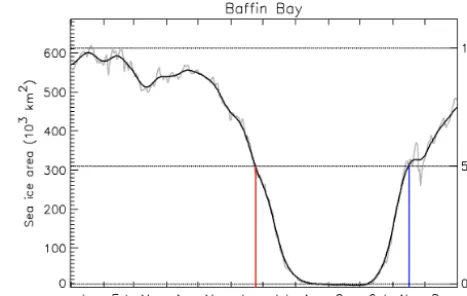
Figure 2.Daily sea-ice area in Baffin Bay (all depths), January– December, 1979–2014 (gray curves). The colored curves are decadal averages, as indicated in the legend. The upper horizontal dotted line (at 613×103km2)is the average sea-ice area in March (1979–2014); the lower horizontal dotted line (at 9×10³km2)is the average sea-ice area in September. The middle horizontal dotted line, halfway between the upper and lower lines, is the threshold for determining the spring and fall transition dates in Baffin Bay. See Fig. S1 for similar plots for other subpopulation regions.
Arctic sea ice typically reaches its maximum area in March and its minimum area in September. Accordingly, we chose the transition threshold for each region as follows. We calculated the mean March sea-ice area over the period 1979–2014, and the mean September sea-ice area over the same period, and then chose the transition threshold to be halfway between these means. This is illustrated for the Baf-fin Bay region in Fig. 2 and for the other regions in Supple-ment Fig. S1. (Figs. 2–9 use Baffin Bay as a sample region for purposes of illustration).
Figure 3 illustrates the method for finding the dates of spring retreat and fall advance in Baffin Bay in one particular year. The daily sea-ice area (gray curve) exhibits small daily fluctuations that can be attributed to the uncertainty in the underlying sea-ice concentration data. We smooth the daily values with a low-pass Gaussian-shaped filter in which 87 % of the weight is within±1 week of the central value (black curve). Then, starting from the minimum sea-ice area in sum-mer, we search forward and backward in time for the first intersections of the smoothed time series with the threshold. The backward search gives the spring date (red vertical line) and the forward search gives the fall date (blue vertical line). Occasionally the smoothed sea-ice area time series may cross the threshold more than once in spring and/or fall. Our method always chooses the crossing date that is closest in time to the summer minimum. In practice, out of 2736 cross-ing dates (36 years×2 seasons×19 regions×2 time series per region), only 131 dates (4.8 %) had any potential for am-biguity. In more than 95 % of the cases there was clearly only a single crossing date.
Figure 3.Determination of the spring and fall transition dates for the year 2005 in Baffin Bay. The gray curve is the daily sea-ice area; the black curve is a smoothed version. The horizontal dotted line (at 311×103km2)is the threshold. The intersection of the threshold with the smoothed (black) curve determines the spring (red) and fall (blue) transition dates.
3.3 Summer sea-ice concentration
For each region we calculated the mean sea-ice concentra-tion for 1 June–31 October for each year, from 1979 to 2014. While it has already been established that the sea-ice concen-tration in every region of the Arctic except the Bering Sea is declining in every month of the year (e.g., Perovich and Richter-Menge, 2009), the winter sea-ice cover will likely continue to provide suitable polar bear habitat for at least several more decades (especially in the Canadian high Arc-tic; Amstrup et al., 2008; Hamilton et al., 2014), whereas the summer sea-ice cover may not. A summer sea-ice metric, therefore, measures the change in polar bear habitat during the season when that habitat is most vulnerable to change. 3.4 Number of ice-covered days per year
We calculated the number of days per year that the sea-ice area in each subpopulation region exceeded the threshold de-fined in Sect. 3.2 (i.e., 50 % of the way from mean September to mean March ice area). For example, in Fig. 3, the sea-ice area in Baffin Bay was greater than the 50 % threshold for 220 days in the year 2005. This sea-ice metric was used as a measure of polar bear habitat in the IUCN Red List assess-ment of polar bears (Wiig et al., 2015).
4 Results
4.1 Sea-ice metrics
Figure 4.Dates of sea-ice retreat (red) and sea-ice advance (blue) in Baffin Bay (all depths) for 1979–2014. The red and blue lines are least-squares fits. The vertical green lines indicate the time interval between retreat and advance (i.e., length of summer season). See Table 3 for trends. See Fig. S2 for similar plots for other regions.
number of ice-covered days per year is decreasing, for the pe-riod 1979–2014 (Table 3). Nearly all the trends (88 of 95) are statistically significant. Trends in the date of spring sea-ice retreat are on the order of−3 to−9 days decade−1(negative being earlier), with the largest trend (−16 days decade−1)in the Barents Sea. Trends in the date of fall sea-ice advance are on the order of+3 to+9 days decade−1(positive being later), with the largest trend (+18 days decade−1)again in the Barents Sea. This means that over the 3.5 decades of this study, the time interval from the date of spring retreat to the date of fall advance has lengthened by 3 to 9 weeks in most regions and by 17 weeks in the Barents Sea. The summer (June–October) sea-ice concentration is declining at a rate of −1 to−9 percent decade−1, depending on region. The num-ber of ice-covered days is declining in all regions at the rate of −7 to−19 days decade−1, with larger trends in the Bar-ents Sea and central Arctic Basin. Results for the shallow (≤300 m) portions of each region are similar (Table 4). Note that some regions consist almost entirely of shallow depths (see Fig. 1 and Table 1).
Figure 4 illustrates results for the Baffin Bay region (see Fig. S2 for similar plots for other regions). Sea-ice re-treat in spring is changing by−7.3 days decade−1(red) and sea-ice advance in fall is changing by +5.4 days decade−1 (blue), both statistically significant. The time interval be-tween the spring and fall transition dates is changing by +12.7 days decade−1(Fig. 5; see Fig. S3 for similar plots for other regions). The summer sea-ice concentration is chang-ing by−4.1 percent decade−1(Fig. 6; see Fig. S4 for similar plots for other regions). The number of ice-covered days is changing by−12.7 days decade−1, which is the negative of the fall-minus-spring trend: the loss of every ice-covered day occurs between the time of spring ice retreat and fall sea-ice advance.
Figure 5.Length of the summer season (from spring sea-ice retreat to fall sea-ice advance) vs. year for Baffin Bay (all depths), with least-squares line in red (slope:+12.7 days decade−1). See Fig. S3 for similar plots for other regions.
Figure 6.Summer (June through October) sea-ice concentration vs. year for Baffin Bay (all depths), with least-squares line in red (slope:
−4.1 percent decade−1). See Fig. S4 for similar plots for other re-gions.
Table 3.Trend in date of spring sea-ice retreat (days decade−1), trend in date of fall sea-ice advance (days decade−1), trend in length of summer season (days decade−1), trend in June–October sea-ice concentration (percent concentration decade−1), trend in number of ice-covered days (days decade−1), and correlation of de-trended dates of spring retreat and fall advance (dimensionless). All quantities are computed from the total marine area of each region, regardless of depth (compare Table 4), for the period 1979–2014. The trend in the length of the summer season (fall–spring trend) is equal to the fall trend minus the spring trend. Statistical significance is indicated by * (95 % level) or ** (99 % level) according to a two-sided F test (for trends) or a two-sidedttest (for correlations).
Subpopulation Spring Fall Fall−spring Jun–Oct Ice-covered Correlation of trend trend trend ice concentration days dates
Kane Basin −6.8 * 5.6 ** 12.4 ** −5.4 ** −14.1 ** −0.55 ** Baffin Bay −7.3 ** 5.4 ** 12.7 ** −4.1 ** −12.7 ** −0.64 ** Lancaster Sound −5.4 * 4.7 ** 10.1 ** −4.4 ** −10.6 ** −0.11
Norwegian Bay −1.2 4.3 5.5 −1.6 −7.1 * −0.21
Viscount Melville −4.0 7.9 11.8 * −4.7 ** −12.3 ** 0.36 * Northern Beaufort −6.0 * 3.1 9.0 * −4.3 ** −9.3 * −0.40 * Southern Beaufort −9.0 ** 8.8 ** 17.8 ** −9.3 ** −17.5 ** −0.50 ** M’Clintock Channel −4.1 ** 5.9 ** 10.0 ** −5.1 ** −11.1 ** −0.74 ** Gulf of Boothia −8.6 ** 7.6 ** 16.2 ** −8.9 ** −18.6 ** −0.57 ** Foxe Basin −5.3 ** 5.7 ** 11.0 ** −3.3 ** −11.4 ** −0.58 ** Western Hudson Bay −5.1 ** 3.5 ** 8.7 ** −2.9 ** −8.6 ** −0.25 Southern Hudson Bay −3.0 * 3.6 * 6.6 ** −1.8 * −6.8 ** −0.35 * Davis Strait −7.4 ** 9.2 ** 16.6 ** −1.0 ** −17.1 ** −0.35 * East Greenland −5.7 ** 4.8 * 10.5 ** −1.4 * −10.4 ** −0.34 * Barents Sea −16.4 ** 18.2 ** 34.6 ** −3.8 ** −41.0 ** −0.46 ** Kara Sea −9.2 ** 7.3 ** 16.5 ** −7.9 ** −16.9 ** −0.49 ** Laptev Sea −6.9 ** 7.0 ** 13.9 ** −9.4 ** −13.5 ** −0.78 ** Chukchi Sea −4.0 ** 5.3 ** 9.3 ** −4.0 ** −8.9 ** −0.39 * Arctic Basin −11.9 ** 15.2 ** 27.1 ** −6.0 ** −24.6 ** 0.35 *
Figure 7.Sea-ice area in Baffin Bay (all depths), 1979–2014. Top green line is mean March sea-ice area; bottom green line is mean September sea-ice area. Two thresholds are shown: 15 and 50 % of the way from the mean September area to the mean March area.
4.2 Correlation of de-trended dates
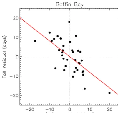
Figure 4 shows that there is year-to-year variability about the trend lines in the dates of spring ice retreat and fall sea-ice advance. Subtracting out the trend lines leaves residuals. We calculated the correlation of the spring residuals with the fall residuals (Table 3, last column). The correlation is neg-ative in most regions, often significantly so. This means that an early spring sea-ice retreat (relative to the trend line) tends to be followed by a late fall sea-ice advance (relative to the
trend line), and vice versa. The de-trended spring and fall dates for Baffin Bay are shown in Fig. 9. The negative corre-lations are likely the result of the ice–albedo feedback, dis-cussed in Sect. 5.4.
Figure 8.Number of ice-covered days in Baffin Bay (all depths), 1979–2014, based on two thresholds: 15 % (blue) and 50 % (red) (see also Fig. 7). Least-squares lines are also shown. See Fig. S5 for similar plots for other regions.
advance (Da)for the current year by extrapolating the his-torical trends (Table 3). (3) In the current year, once the date of spring sea-ice retreat has been observed (Drobs), predict the date of fall sea-ice advance as Da+S×(Dobsr −Dr). This is the date projected by the trend line plus the anomaly predicted by the historical correlation of the spring and fall dates. This method should give several months of lead time for the predicted date of fall sea-ice advance, with a higher degree of skill than simply predicting a continuation of the fall linear trend, in those regions where the spring and fall dates are significantly correlated.
4.3 Spatial patterns
The spatial pattern of trends in the date of spring sea-ice re-treat (Fig. 10) shows that all trends over shallow depths are statistically significant except in the Northern Beaufort, Vis-count Melville, and Norwegian Bay regions. Otherwise, the continental shelves around the Arctic show significantly ear-lier spring retreat, generally −3 to −9 days decade−1, with faster retreat in the northern Chukchi and East Siberian seas, Kane Basin, and especially the Barents Sea. For the date of fall sea-ice advance (Fig. 11), all regions have positive trends, but the trends are not statistically significant in some parts of the Canadian Arctic Archipelago. The rest of the continental shelf regions around the Arctic show significantly later fall advance, generally 3 to 9 days decade−1, with larger rates in the northern Chukchi and East Siberian seas and in the Bar-ents Sea, similar to the spring pattern. The increase in the length of the summer season (Fig. 12) shows the same pat-tern, with roughly double the rate (since it equals the fall rate minus the spring rate).
Note that in this analysis, the Chukchi Sea region extends south of Bering Strait into the northern Bering Sea. We know from other analyses (e.g., Laidre et al., 2015a; Parkinson, 2014) that there has been a slight increase in sea ice in the
Bering Sea. Therefore the negative trends for the Chukchi Sea reported here, while still statistically significant, are rel-atively small because of the inclusion of the northern Bering Sea within the Chukchi Sea region. Similarly, the trends for the Arctic Basin region are relatively large because that re-gion includes the northern Chukchi Sea, where summer sea ice has been rapidly disappearing (e.g., Frey et al., 2015; Parkinson, 2014).
4.4 Sensitivity to threshold
The calculation of the spring and fall transition dates is based on a sea-ice area threshold that is halfway between the mean September sea-ice area and the mean March sea-ice area for each region. Different thresholds would lead to different tran-sition dates. How sensitive are the trantran-sition dates to the ac-tual choice of threshold? The answer can be seen in Fig. 2 (and Fig. S1). The rate of change of sea-ice area (i.e., its slope) is relatively steep at the times of threshold crossing, indicating that sea ice diminishes quickly in spring and grows back quickly in fall compared to the rate of change in winter and summer. Therefore the transition dates are relatively in-sensitive to the threshold, in the sense that a small change in the threshold would lead to a small change in the transition dates.
5 Discussion
5.1 Previous studies of the timing of Arctic sea-ice advance and retreat
Many studies in the last 10 years have considered changes in the timing of sea-ice advance and retreat in the con-text of polar bear ecology. Stirling and Parkinson (2006) used daily sea-ice concentration from satellite passive mi-crowave data to calculate the date of sea-ice breakup (50 % concentration) in spring in Baffin Bay for each year from 1979 through 2004, finding a statistically significant trend toward earlier breakup (−6.6±2.0 days decade−1). The tim-ing of polar bear onshore arrival in western Hudson Bay was previously shown to be significantly related to the 50 % sea-ice concentration threshold (Stirling et al., 1999). Other studies of sea-ice timing and polar bears include Regehr et al. (2007), Obbard et al. (2007), Hamilton et al. (2014), Lunn et al. (2014), Laidre et al. (2015a), and Obbard et al. (2016). These studies are summarized in Table 2, along with eight other studies where sea-ice metrics were used for analysis of polar bear habitat.
encom-Figure 9.Date of fall sea-ice advance (de-trended) vs. date of spring sea-ice retreat (trended) for Baffin Bay (all depths). The de-trended dates have correlation−0.64. This suggests that the date of fall ice advance can be predicted from the date of spring sea-ice retreat with more skill than simply extrapolating the fall trend. See Table 3 for correlations in all regions. The red line is the least-squares fit.
passing parts of the East Siberian/Chukchi/Beaufort seas and the Kara/Barents seas. Dates of sea-ice retreat in these re-gions trended earlier by 15–18 days decade−1, and dates of sea-ice advance trended later by 10–13 days decade−1, with correlations of de-trended dates on the order of−0.8. Their results are slightly more extreme than ours (Table 3) because their regions were specifically tailored to include the largest trends, but our results are nevertheless generally consistent with theirs.
Parkinson (2014) used daily passive microwave data (1979–2013) to calculate and map the number of days per year with sea-ice concentration ≥ 15 %, finding that most of the Arctic seasonal ice zone (roughly all regions in Fig. 1 except the Arctic Basin) is experiencing a loss of 10– 20 days decade−1, with the most rapid loss in the Barents Sea. They also found that the trends are not sensitive to the 15 % threshold, with similar trends obtained using 50 %. The results are consistent with ours (Table 3) that show a decrease in the number of ice-covered days.
Frey et al. (2015) used daily passive microwave data (1979–2012) to study the timing of sea-ice breakup, freeze-up, and persistence in the Beaufort, Chukchi, and Bering seas, finding trends toward earlier breakup and later freeze-up in the Beaufort and Chukchi seas, with steeper trends since 2000. They also used wind and air temperature data to determine that for the localized areas that are experienc-ing the most rapid shifts in sea ice, those in the Beaufort Sea are primarily wind driven, while those offshore in the Canada Basin are primarily thermally driven.
Figure 10.Trend map of the date of spring sea-ice retreat for the shallow parts of each PBSG region. Trends are also given in Table 4.
Steele et al. (2015) looked at the timing of sea-ice retreat in the southeastern and southwestern Beaufort Sea using daily sea-ice concentration data (1979–2012). They found no trend in the date of retreat in the southeastern Beaufort Sea but did find a trend toward earlier retreat in the southwestern Beau-fort Sea. Furthermore, an increase in monthly mean easterly winds of∼1 m s−1during spring was associated with an ear-lier summer sea-ice retreat of 6–15 days, offering predictive capability of sea-ice retreat with 2 to 4 months of lead time.
Our methods in the present study are based on our pre-vious work. Laidre et al. (2015a) calculated the timing of sea-ice advance and retreat in 12 Arctic regions (1979–2013) for the Conservation of Arctic Flora and Fauna (CAFF) Arc-tic Biodiversity Assessment (ABA). Laidre et al. (2015b) focused on polar bear habitat in East Greenland, including changes in the timing of sea-ice advance and retreat. Laidre et al. (2012) examined narwhal sea-ice entrapments and the timing of fall sea-ice advance in six narwhal summering ar-eas of Baffin Bay. Heide-Jørgensen et al. (2013) considered changes in the timing of spring sea-ice retreat in the North Water Polynya. All these studies found trends toward earlier spring sea-ice retreat and later fall sea-ice advance from the 1980s to present.
Figure 11.Trend map of the date of fall sea-ice advance for the shallow parts of each PBSG region. Trends are also given in Table 4.
sea-ice advance, and summer (June–October) sea-ice con-centration for each of the 19 polar bear subpopulations, as reported here, and will be updated accordingly. The IUCN Red List assessment of polar bears (Wiig et al., 2015) used the number of ice-covered days per year as its sea-ice metric, as presented here in Sect. 3.4.
5.2 Relevance to other Arctic marine mammal species
While the metrics reported here were tailored specifically to polar bears and polar bear ecology, they can be considered relevant for a range of other AMM species. Besides the polar bear, AMMs are typically considered to be three cetacean species (the narwhal, Monodon monoceros; beluga, Del-phinapterus leucas; and bowhead whale, Balaena mystice-tus) and seven pinniped species (the ringed seal,Pusa hisp-ida; bearded seal,Erignathus barbatus; spotted seal,Phoca largha; ribbon seal, Phoca fasciata; harp seal, Pagophilus groenlandicus; hooded seal, Cystophora cristata; and wal-rus,Odobenus rosmarus) (Laidre et al., 2008; Laidre et al., 2015a). These species all occur north of the Arctic Circle for most of the year and depend on the Arctic marine ecosystem for all aspects of life. In a few cases some may live outside the Arctic for part of the year. All depend on the timing of sea-ice advance and retreat for different aspects of their life history, and thus the metrics in this study may be relevant to understanding changes in the regions where these AMMs occur.
Figure 12.Trend map of the length of the summer season for the shallow parts of each PBSG region. Trends are also given in Table 4.
5.3 Variability in the timing of sea-ice advance and retreat
The dates of sea-ice advance and retreat, as shown in Figs. 4 and S2, vary about the trend lines. Some regions such as East Greenland have high year-to-year variability, while other re-gions such as Foxe Basin have low year-to-year variability (as measured, for example, by the standard deviation of the residuals about the trend line). The high variability is likely due to advection of sea ice through the region due to wind and currents, while the low variability indicates a lack of such advection, as noted by Laidre et al. (2012), who found that three sheltered sites on the western side of Baffin Bay had low variability in fall freeze-up dates, while sites near the North Water Polynya in northern Baffin Bay, and in the East Greenland Current, had high variability. In regions where sea-ice advance and retreat are primarily driven by thermo-dynamics, the year-to-year variability will be lower than in regions where wind and currents are strong.
5.4 Correlation of dates of sea-ice retreat and advance
Table 4.Same as Table 3 but for the shallow (≤300 m) portions of each region.
Subpopulation Spring Fall Fall–spring Jun–Oct Ice-covered Correlation of trend trend trend ice concentration days dates
Kane Basin −9.7 ** 5.5 ** 15.2 ** −6.9 ** −15.1 ** −0.36 * Baffin Bay −8.4 ** 9.7 ** 18.1 ** −3.3 ** −19.8 ** −0.54 ** Lancaster Sound −7.6 ** 4.6 ** 12.2 ** −4.3 ** −11.2 ** −0.35 *
Norwegian Bay −1.3 4.2 5.5 −1.6 −7.0 ** −0.21
Viscount Melville −4.3 6.9 11.2 * −4.3 ** −11.7 ** 0.31 Northern Beaufort −5.6 3.5 ** 9.1 * −3.6 * −8.5 * −0.62 ** Southern Beaufort −7.3 ** 8.6 ** 15.9 ** −7.9 ** −15.5 ** −0.53 ** M’Clintock Channel −4.1 ** 5.8 ** 10.0 ** −5.2 ** −11.0 ** −0.74 ** Gulf of Boothia −8.6 ** 7.6 ** 16.2 ** −9.0 ** −18.8 ** −0.57 ** Foxe Basin −5.2 ** 5.6 ** 10.9 ** −3.2 ** −11.3 ** −0.57 ** Western Hudson Bay −5.1 ** 3.5 ** 8.7 ** −2.9 ** −8.6 ** −0.25 Southern Hudson Bay −3.0 * 3.6 * 6.6 ** −1.8 * −6.8 ** −0.35 Davis Strait −6.9 ** 8.0 ** 14.9 ** −1.9 ** −14.7 ** −0.26 East Greenland −4.5 ** 4.6 ** 9.0 ** −3.0 * −9.4 ** −0.30 Barents Sea −17.0 ** 21.0 ** 37.9 ** −4.2 ** −44.6 ** −0.46 ** Kara Sea −8.8 ** 7.0 ** 15.8 ** −7.3 ** −16.2 ** −0.47 ** Laptev Sea −6.8 ** 6.5 ** 13.3 ** −9.1 ** −13.2 ** −0.77 ** Chukchi Sea −4.1 ** 5.4 ** 9.5 ** −4.1 ** −9.1 ** −0.39 * Arctic Basin −9.4 ** 16.8 ** 26.1 ** −9.0 ** −29.3 ** −0.18
sea ice can begin to form, thus delaying fall freeze-up. Con-versely, a late spring sea-ice retreat prevents the ocean from absorbing as much heat, allowing sea ice to form earlier in the fall (e.g., Perovich et al., 2007). The negative correlations are not perfect because other factors contribute to the timing of sea-ice retreat and advance, such as short-term weather events and long-term climate patterns. This is also discussed in more detail by Blanchard et al. (2011), who attributed the “re-emergence of memory” in the fall to the several-month persistence of sea surface temperatures (SSTs) over the sum-mer, enhanced by the ice–albedo feedback. We calculated the correlation of the date of fall sea-ice advance in yearnwith the date of spring sea-ice retreat in yearn+1, but the corre-lation was not significant in any region, suggesting that SST anomalies do not persist through the winter.
5.5 Sea-ice area vs. extent
Some sea-ice studies use sea-ice extent, rather than sea-ice area, to characterize sea-ice coverage. Sea-ice extent is the total area of all grid cells with sea-ice concentration greater than 15 %, i.e., not weighted by the sea-ice concentration. If the sea-ice concentration in a grid cell exceeds 15 %, the entire area of the grid cell counts toward the sea-ice extent. This is useful in some contexts, but we believe that sea-ice area is a better measure of how much usable sea ice is actu-ally present for polar bears. Also, sea-ice extent is a highly nonlinear function of sea-ice concentration, which leads to more abrupt jumps in its time series than sea-ice area.
5.6 Melt onset and freeze-up
Some investigators have approached the idea of seasonal transitions in the Arctic by examining the dates of melt onset in the spring and freeze-up in the fall, based on the presence of liquid water in the surface layer of the ice or snow (Wine-brenner et al., 1994, 1996; Smith, 1998; Belchansky et al., 2004; Markus et al., 2009; Stroeve et al., 2014). In these stud-ies, melt onset and freeze-up are closely tied to the surface air temperature, but they are not indicators of sea-ice cover-age or condition. For example, at the SHEBA station in the Beaufort Sea in 1997–1998 (Perovich et al., 1999), melt on-set occurred on 29 May when rain fell, but the sea ice did not actually break up until the end of July when a storm passed through. Similarly in fall, melt ponds on the surface of the ice began to freeze in mid-August but the sea ice did not actu-ally consolidate into winter-like pack ice until early October (Stern and Moritz, 2002). Melt onset and freeze-up dates are useful as climate metrics, but for ice-dependent marine mam-mals, transition dates between seasons are best measured by the sea-ice coverage itself, rather than proxies tied to air tem-perature.
5.7 National Climate Assessment (NCA)
the present study was to develop a sea-ice climate metric (or indicator) with relevance to marine mammals that could be used in future NCA reports. The timing of sea-ice advance and retreat satisfies all the qualifications for climate indica-tors put forward by the NCA (NCA, 2011).
6 Conclusions
It is well established that the area of Arctic sea ice is declin-ing in all months of the year, based on satellite passive mi-crowave data from 1979 to the present (Fetterer et al., 2016; IPCC, 2013). In this study we looked instead at the timing of sea-ice retreat in spring and advance in fall, because the dura-tion of the sea-ice season (or equivalently the ice-free season) is important for polar bears. We found that there has been a consistent and large loss of habitat for polar bears across the Arctic. In 17 of the 19 subpopulation regions there are sig-nificant trends toward earlier spring sea-ice retreat, mostly ranging from −3 to−9 days decade−1. In 16 of the regions there are significant trends toward later fall sea-ice advance, mostly ranging from+3 to+9 days decade−1. Over the 3.5 decades of this study, the time interval from the date of spring retreat to the date of fall advance has lengthened by 3 to 9 weeks in most regions.
General circulation models (GCMs) predict ice-free Arc-tic summers by mid-century or sooner (IPCC, 2013; Over-land and Wang, 2013). Spring sea-ice retreat will continue to arrive earlier and fall sea-ice advance will continue to ar-rive later, with no reversal in sight. Barnhart et al. (2015) used daily sea-ice output from a 30-member GCM ensem-ble, driven by the business-as-usual emissions scenario (RCP 8.5), to map the annual duration of open water in the Arc-tic through 2100. They found that by 2050 the entire ArcArc-tic coastline and most of the Arctic Ocean will experience an additional 1 to 2 months of open water per year, relative to present conditions, which is consistent with extrapolation of the trends in Table 3.
What are the implications of these physical changes for the global population of polar bears? Their dependence on sea-ice means that climate warming poses the single most important threat to their persistence (Stirling and Derocher, 2012; USFWS, 2013). Changes in sea ice have been shown to impact polar bear abundance, productivity, body condition, and distribution (Stirling et al., 1999; Durner et al., 2009; Regehr et al., 2010; Rode et al., 2012, 2014; Bromaghin et al., 2015; Obbard et al., 2016). Furthermore, population and habitat models predict substantial declines in the distribution and abundance of polar bears in the future (Durner et al., 2009; Amstrup et al., 2008; Castro de la Guardia et al., 2013; Hamilton et al., 2014). This study offers standardized metrics with which to compare polar bear habitat change across the 19 subpopulations and provides a starting point for including sea-ice habitat change in circumpolar polar bear management and conservation plans.
The Supplement related to this article is available online at doi:10.5194/tc-10-2027-2016-supplement.
Author contributions. Harry L. Stern carried out the sea-ice calcu-lations in consultation with Kristin L. Laidre; Harry L. Stern and Kristin L. Laidre prepared the manuscript.
Acknowledgements. This work was supported by NASA under the programs Development and Testing of Potential Indicators for the National Climate Assessment, grant NNX13AN28G (PI: Harry L. Stern), and Climate and Biological Response, grant NNX11A063G (PI: Kristin L. Laidre). We also acknowledge support from the Greenland Institute of Natural Resources. We thank the National Snow and Ice Data Center in Boulder for sea-ice concentration data, and NOAA for bathymetry data (ETOPO1). We thank Eric Regehr, Steve Amstrup, and Cecilia Bitz for conversations about sea-ice metrics. We thank the PBSG for input during the development of the metrics. We thank Andy Derocher and one anonymous reviewer for comments that helped to improve the paper.
Edited by: C. Haas
Reviewed by: two anonymous referees
References
Amante, C. and Eakins, B. W.: ETOPO1 1 Arc-Minute Global Relief Model: Procedures, Data Sources and Analysis, NOAA Technical Memorandum NESDIS NGDC-24, National Geophys-ical Data Center, NOAA, doi:10.7289/V5C8276M, 2009. Amstrup, S. C., Marcot, B. G., and Douglas, D. C.: A Bayesian
net-work modeling approach to forecasting the 21st century world-wide status of polar bears, in: Arctic Sea Ice Decline: Obser-vations, Projections, Mechanisms and Implications, edited by: DeWeaver, E. T., Bitz, C. M., and Tremblay, L. B., Geophysical Monograph Series 180, American Geophysical Union, Washing-ton, DC, USA, 213–268, 2008.
Barnhart, K. R., Miller, C. R., Overeem, I., and Kay, J. E.: Map-ping the future expansion of Arctic open water, Nature Climate Change, 6, 280–285, doi:10.1038/NCLIMATE2848, 2015. Belchansky, G. I., Douglas, D. C., and Platonov, N. G.: Duration of
the Arctic Sea Ice Melt Season: Regional and Interannual Vari-ability, 1979–2001, J. Climate, 17, 67–80, 2004.
Blanchard, E., Armour, K. C., and Bitz, C. M.: Persis-tence and Inherent Predictability of Arctic Sea Ice in a GCM Ensemble and Observations, J. Climate, 24, 231–250, doi:10.1175/2010JCLI3775.1, 2011.
Castro de la Guardia, L., Derocher, A. E., Myers, P. G., Terwisscha van Scheltinga, A. D., and Lunn, N. J.: Future sea ice conditions in Western Hudson Bay and consequences for polar bears in the 21st century, Glob. Change Biol., 19, 2675–2687, 2013. Cavalieri, D. J., Parkinson, C. L., Gloersen, P., and Zwally, H. J.: Sea
Ice Concentrations from Nimbus-7 SMMR and DMSP SSM/I-SSMIS Passive Microwave Data, Version 1, Boulder, Colorado USA, NASA National Snow and Ice Data Center Distributed Active Archive Center, doi:10.5067/8GQ8LZQVL0VL, updated yearly, 1996.
Cherry, S. G., Derocher, A. E., Thiemann, G. W., and Lunn, N. J.: Migration phenology and seasonal fidelity of an Arctic marine predator in relation to sea ice dynamics, J. Animal Ecology, 82, 912–921, doi:10.1111/1365-2656.12050, 2013.
Durner, G. M., Douglas, D. C., Nielson, R. M., Amstrup, S. C., McDonald, T. L., Stirling, I., Mauritzen, Born, E. W., Wiig, Ø., DeWeaver, E. T., Serreze, M. C., Belikov, S. E., Holland, M. M., Maslanik, J., Aars, J., Bailey, D. A., and Derocher, A. E.: Predict-ing 21st-century polar bear habitat distribution from global cli-mate models, Ecol. Monogr., 79, 25–58, doi:10.1890/07-2089.1, 2009.
Fetterer, F., Knowles, K., Meier, W., and Savoie, M.: Sea Ice Index, updated daily, Boulder, Colorado USA: National Snow and Ice Data Center, doi:10.7265/N5QJ7F7W, 2016.
Frey, K. E., Moore, G. W. K., Cooper, L. W., and Grebmeier, J. M.: Divergent patterns of recent sea ice cover across the Bering, Chukchi, and Beaufort seas of the Pacific Arctic Region, Prog. Oceanogr., 136, 32–49, 2015.
Hamilton, S. G., Castro de la Guardia, L., Derocher, A. E., Saha-natien, V., and Tremblay, B.: Projected Polar Bear Sea Ice Habi-tat in the Canadian Arctic Archipelago, PLoS ONE, 9, e113746, doi:10.1371/journal.pone.0113746, 2014.
Heide-Jørgensen, M. P., Burt, M. L., Hansen, R. G., Nielsen, N. H., Rasmussen, M., Fossette, S., and Stern, H.: The Significance of the North Water Polynya to Arctic Top Predators, AMBIO, 42, 596–610, doi:10.1007/s13280-012-0357-3, 2013.
IPCC: Climate Change 2013: The Physical Science Basis, in: Con-tribution of Working Group I to the Fifth Assessment Report of the Intergovernmental Panel on Climate Change, edited by: Stocker, T. F., Qin, D., Plattner, G.-K., Tignor, M., Allen, S. K., Boschung, J., Nauels, A., Xia, Y., Bex, V., and Midgley, P. M., Cambridge University Press, Cambridge, United Kingdom and New York, NY, USA, 1535 pp., 2013.
Ivanova, N., Pedersen, L. T., Tonboe, R. T., Kern, S., Heyg-ster, G., Lavergne, T., Sørensen, A., Saldo, R., Dybkjær, G., Brucker, L., and Shokr, M.: Inter-comparison and evaluation of sea ice algorithms: towards further identification of chal-lenges and optimal approach using passive microwave obser-vations, The Cryosphere, 9, 1797–1817, doi:10.5194/tc-9-1797-2015, 2015.
Laidre, K. L., Stern, H., Kovacs, K. M., Lowry, L., Moore, S., Regehr, E. V., Ferguson, S., Wiig, Ø., Boveng, P., Angliss, R. P., Born, E. W., Litovka, D., Quakenbush, L., Lydersen, C., Vongraven, D., and Ugarte, F.: Arctic marine mammal pop-ulation status, sea ice habitat loss, and conservation recom-mendations for the 21st century, Conserv. Biol., 29, 724–737, doi:10.1111/cobi.12474, 2015a.
Laidre, K. L., Born, E. W., Heagerty, P., Wiig, Ø., Stern, H., Dietz, R., Aars, J., and Andersen, M.: Shifts in female polar bear (Ursus
maritimus) habitat use in East Greenland, Polar Biol., 38, 879– 893, doi:10.1007/s00300-015-1648-5, 2015b.
Laidre, K., Heide-Jørgensen, M. P., Stern, H., and Richard, P.: Un-usual narwhal sea ice entrapments and delayed autumn freeze-up trends, Polar Biol., 35, 149–154, doi:10.1007/s00300-011-1036-8, 2012.
Laidre, K. L., Stirling, I., Lowry, L., Wiig, Ø., Heide-Jørgensen, M. P., and Ferguson, S.: Quantifying the sensitivity of arctic ma-rine mammals to climate-induced habitat change, Ecol. Appl., 18, S97–S125, 2008.
Lunn, N., Servanty, S., Regehr, E., Converse, S., Richardson, E., and Stirling, I.: Demography and population status of polar bears in Western Hudson Bay, Environment Canada research report, 2014.
Markus, T., Stroeve, J. C., and Miller, J.: Recent changes in Arctic sea ice melt onset, freezeup, and melt season length, J. Geophys. Res., 114, C12024, doi:10.1029/2009JC005436, 2009.
Melillo, J. M., Terese, T. C. R., and Gary, W. Y. (Eds.): Climate Change Impacts in the United States: The Third National Cli-mate Assessment, US Global Change Research Program, 841 pp. doi:10.7930/J0Z31WJ2, 2014.
NCA: The United States National Climate Assessment, NCA Re-port Series, Volume 5b, Monitoring Climate Change and its Im-pacts: Physical Climate Indicators, 32 pp., 2011.
NSIDC: Documentation at: http://nsidc.org/data/docs/daac/ nsidc0051_gsfc_seaice.gd.html, 2015.
Obbard, M., McDonald, T. L., Howe, E. J., Regehr, E. V., and Richardson, E. S.: Polar Bear Population Status in Southern Hud-son Bay, Canada, USGS Administrative report, 2007.
Obbard, M. E., Thiemann, G. W., Peacock, E., and DeBruyn, T. D. (Eds.): Polar Bears: Proceedings of the 15th Working Meet-ing of the IUCN/SSC Polar Bear Specialist Group, Copenhagen, Denmark, 29 June–3 July 2009, IUCN, Gland, Switzerland and Cambridge, UK, 235 pp., 2010.
Obbard, M. E., Cattet, M. R. L., Howe, E. J., Middel, K. R., Newton, E. J., Kolenosky, G. B., Abraham, K. F., and Greenwood, C. J.: Trends in body condition in polar bears (Ursus maritimus) from the Southern Hudson Bay subpopulation in relation to changes in sea ice, Arct. Sci., 2, 15–32, doi:10.1139/as-2015-0027, 2016. Overland, J. E. and Wang, M.: When will the summer Arctic be nearly sea ice free?, Geophys. Res. Lett., 40, 2097–2101, doi:10.1002/grl.50316, 2013.
Paetkau, D., Amstrup, S. C., Born, E .W., Calvert, W., Derocher, A. E., Garner, G. W., Messier, F., Stirling, I., Taylor, M. K., Wiig, Ø., and Strobeck, C.: Genetic structure of the world’s polar bear populations, Molecular Ecol., 8, 1571–1584, 1999.
Parkinson, C. L.: Spatially mapped reductions in the length of the Arctic sea ice season, Geophys. Res. Lett., 41, 4316–4322, doi:10.1002/2014GL060434, 2014.
Parkinson, C. L. and Cavalieri, D. J.: Arctic sea ice variabil-ity and trends, 1979–2006, J. Geophys. Res., 113, C07003, doi:10.1029/2007JC004558, 2008.
Peacock, E., Laake, J., Laidre, K. L., Born, E., and Atkinson, S.: The utility of harvest recoveries of marked individuals to assess polar bear (Ursus maritimus) survival, Arctic, 65, 391–400, 2012. Peacock, E., Taylor, M. K., Laake, J., and Stirling, I.: Population
Peacock, E., Sonsthagen, S. A., Obbard, M. E., Boltunov, A., Regehr, E. V., Ovsyanikov, N., Aars, J., Atkinson, S. N., Sage, G. ., Hope, A. G., Zeyl, E., Bachmann, L., Ehrich, D., Scribner, K. T., Amstrup, S. C., Belikov, S., Born, E. W., Derocher, A. E., Stirling, I., Taylor, M. K., Wiig, Ø., Paetkau, D., and Talbot, S. L.: Implications of the circumpolar genetic structure of polar bears for their conservation in a rapidly warming Arctic, PLoS ONE, 10, e11202, doi:10.1371/journal.pone.0112021, 2015. Perovich, D. K. and Richter-Menge, J. A.: Loss of Sea Ice in the
Arctic, Annu. Rev. Mar. Sci., 1, 417–441, 2009.
Perovich, D. K., Light, B., Eicken, H., Jones, K. F., Runciman, K., and Nghiem, S. V.: Increasing solar heating of the Arc-tic Ocean and adjacent seas, 1979–2005: Attribution and role in the ice-albedo feedback, Geophys. Res. Lett., 34, L19505, doi:10.1029/2007GL031480, 2007.
Perovich, D. K., Andreas, E. L., Curry, J. A., Eiken, H., Fairall, C. W., Grenfell, T. C., Guest, P. S., Intrieri, J., Kadko, D., Lindsay, R. W., McPhee, M. G., Morison, J., Moritz, R. E., Paulson, C. A., Pegau, W. S., Persson, P. O. G., Pinkel, R., Richter-Menge, J. A., Stanton, T., Stern, H., Sturm, M., Tucker III, W. B., and Uttal, T.: Year on Ice Gives Climate Insights, Eos, Transactions, American Geophysical Union, 80, 41, 485–486, 1999.
Regehr, E. V., Lunn, N. J., Amstrup, S. C., and Stirling, I.: Effects of earlier sea ice breakup on survival and population size of polar bears in western Hudson Bay, J. Wildlife Manage., 71, 2673– 2683, doi:10.2193/2006-180, 2007.
Regehr, E. V., Hunter, C. M., Caswell, H., Amstrup, S. C., and Stirling, I.: Survival and breeding of polar bears in the southern Beaufort Sea in relation to sea-ice, J. Animal Ecol., 79, 117–127, 2010.
Regehr, E. V., Wilson, R. R., Rode, K. D., and Runge, M. C.: Re-silience and risk – A demographic model to inform conservation planning for polar bears, US Geological Survey Open-File Re-port 2015–1029, 56 pp., doi:10.3133/ofr20151029, 2015. Rode, K. D., Peacock, E., Taylor, M., Stirling, I., Born, E. W.,
Laidre, K. L., and Wiig, Ø.: A tale of two polar bear populations: Ice habitat, harvest, and body condition, Population Ecology, 54, 3–18, doi:10.1007/s10144-011-0299-9, 2012.
Rode, K. D., Regehr, E. V., Douglas, D. C., Durner, G., Derocher, A. E., Thiemann, G. W., and Budge, S. M.: Variation in the response of an Arctic top predator experiencing habitat loss: feeding and reproductive ecology of two polar bear populations, Glob. Change Biol., 20, 76–88, 2014.
Smith, D. M.: Recent increase in the length of the melt season of perennial Arctic sea ice, Geophys. Res. Lett., 25, 655–658, 1998. Stammerjohn, S., Massom, R., Rind, D., and Martinson, D.: Regions of rapid sea ice change: An inter-hemispheric seasonal comparison, Geophys. Res. Lett., 39, L06501, doi:10.1029/2012GL050874, 2012.
Steele, M., Dickinson, S., Zhang, J., and Lindsay, R.: Sea-sonal ice loss in the Beaufort Sea: Toward synchrony and prediction, J. Geophys. Res.-Oceans, 120, 1118–1132, doi:10.1002/2014JC010247, 2015.
Stern, H. L. and Moritz, R. E.: Sea ice kinematics and sur-face properties from RADARSAT synthetic aperture radar during the SHEBA drift, J. Geophys. Res., 107, 8028, doi:10.1029/2000JC000472, 2002.
Stirling, I. and Derocher, A. E.: Effects of climate warming on polar bears: a review of the evidence, Glob. Change Biol., 18, 2694– 2706, doi:10.1111/j.1365-2486.2012.02753.x, 2012.
Stirling, I. and Parkinson, C. L.: Possible Effects of Climate Warm-ing on Selected Populations of Polar Bears (Ursus maritimus) in the Canadian Arctic, Arctic, 59, 261–275, 2006.
Stirling, I., Lunn, N. J., and Iacozza, J.: Long-term trends in the pop-ulation ecology of polar bears in western Hudson Bay in relation to climatic change, Arctic, 52, 294–306, 1999.
Stirling, I., McDonald, T., Richardson, E. S., Regehr, E. V., and Am-strup, S.: Polar bear population status in the northern Beaufort Sea, Canada, 1971–2006, Ecol. Appl., 21, 859–876, 2011. Stroeve, J. C., Serreze, M. C., Holland, M. M., Kay, J. E., Malanik,
J., and Barrett, A. P.: The Arctic’s rapidly shrinking sea ice cover: a research synthesis, Climatic Change, 110, 1005–1027, 2012. Stroeve, J. C., Markus, T., Boisvert, M., and Barrett, A.: Changes
in Arctic melt season and implications for sea ice loss, Geophys. Res. Lett., 41, 1216–1225, doi:10.1002/2013GL058951, 2014. US Fish and Wildlife Service (USFWS): Endangered and
Threat-ened Wildlife and Plants; Special Rule for the Polar Bear Under Section 4(d) of the Endangered Species Act, Federal Register 78, 34, 11766–11788, Washington, D.C., USA, 2013.
Vongraven, D., Aars, J., Amstrup, S., Atkinson, S. N., Belikov, S., Born, E. W., DeBruyn, T. D., Derocher, A. E., Durner, G., Gill, M., Lunn, N., Obbard, M. E., Omelak, J., Ovsyanikov, N., Pea-cock, E., Richardson, E., Sahanatien, V., Stirling, I., and Wiig, Ø.: A circumpolar monitoring framework for polar bears, Ursus, Vol. 23, Special Issue: Monograph Series Number 5, 1–66, 2012. Wiig, Ø., Amstrup, S., Atwood, T., Laidre, K., Lunn, N., Ob-bard, M., Regehr, E., and Thiemann, G.: Polar Bear (Ursus maritimus), The IUCN Red List of Threatened Species 2015, doi:10.2305/IUCN.UK.2015-4.RLTS.T22823A14871490.en, 2015.
Winebrenner, D. P., Holt, B., and Nelson, E. D.: Observation of au-tumn freeze-up in the Beaufort and Chukchi Seas using the ERS 1 synthetic aperture radar, J. Geophys. Res., 101, 16401–16419, 1996.