Optimization of Surplus Reinsurance Treaty using the Conditional Tail Expectation

(1)

using the Conditional Tail Expectation

El Attar Abderrahim Department of Mathematics

Mohamed V University, Faculty of Sciences-Rabat, Morocco estimabd@hotmail.com

El Hachloufi Mostafa

Department of Statistics and Mathematics Applied to Economics and Management Faculty of Juridical Sciences, Economic and Social-Ain Sebaa, Morocco

elhachloufi@yahoo.fr

Guennoun Zine El Abidine Department of Mathematics

Mohamed V University, Faculty of Sciences-Rabat, Morocco guennoun@fsr.ac.ma

Abstract

In this work, we propose a new optimization strategy for reinsurance using the genetic algorithms. This approach is to determine an optimal structure of a "surplus" reinsurance contract by finding the optimal cession rates through an optimization model which is based on the minimization of the Conditional Tail Expectation (CTE) risk measure under the constraint of technical benefit. This approach can be seen as a decision support tool that can be used by managers to minimize the actuarial risk and maximize the technical benefit in the insurance company.

Keywords: Augmented Lagrangian; Cession rate; Conditional Tail Expectation; Genetic algorithms; Reinsurance; Technical benefit.

1. Introduction

(2)

In the previous approaches, the authors applied a premium principle (pricing mode) based on mathematical expectation. Gajeck and Zagrodny [20] and Kaluszka [25] studied the same approach using the other bonus principles based on variance.This study results in an optimal reinsurance treaty that mixes the "quote share" and the "loss surplus" called "change-loss reinsurance". Walhin and Lampaert [38] applied the mean-variance approach to the form of proportional reinsurance of the "surplus" type. However, several criticisms were addressed to these models, such as the choice of variance as a measure of risk and the burden of computation. These criticisms give rise to a multitude of attempts to improve these models or to develop new models. In this light, many researchers have proposed new criteria for the optimal choice of reinsurance, there are, among others, Dickson and Waters [18], Aase [1], Krvavych [26], Deelstra and Plantin [15] who have chosen optimality by the minimization criterion of the probability of ruin while justifying this choice. However, several authors such as Ben Dbabis [7] have verified that the criterion of minimizing the probability of ruin alone does not lead to a rational decision for an optimal choice of reinsurance, because this criterion acts only on the risk (by minimizing the probability of ruin), but it does not act on the technical benefit, ie the insurer must not choose the optimal reinsurance treaty if it is not profitable.

For this reason, several researchers have introduced a new criterion for choosing optimal reinsurance based on the minimization of risk measures, such as Value-at-Risk (VaR) and Conditional Tail Expectation (CTE). This criterion was introduced by Cai and Tan [12] who disassembled the existence of explicit optimal retention in the case of "stop loss" treaty. The Cai and Tan [12] approach was then generalized by Tan and Chi [37] who used an auxiliary model to solve the optimal reinsurance treaty problem using the "CTE-minimization" model.

The various previous approaches that have started the literature on the problem of optimizing reinsurance, act either on the technical benefit (by maximizing it for a given risk), or on the risk (by minimizing it for a given technical benefit), but they do not act on both at the same time in a dynamic way. In fact, the use of the preceding optimization criteria alone does not generally lead to a rational decision, for the choice of optimal reinsurance. That is, minimizing risk does not always imply maximum technical benefit, and vice versa. So the insurer should not choose the optimal reinsurance treaty if it is not beneficial.

In this context, we have proposed practical solution for determining the optimal "surplus" reinsurance treaty through minimizing Conditional Tail Expectation risk measure under technical benefit constraints. In addition we have created an optimization procedure based on the Augmented Lagrangian method and the Genetic Algorithms to solve the optimization problem of this model.

(3)

2. Conditional Tail Expectation (CTE)

Definition 1. The Conditional Tail Expectation (CTE) is a measure of risk corresponding to a random variable X at the probability level 

 

0,1 , denoted by

( )

CTE X_ and defined by:

 

( )

CTE X_ E X X_ VaR_ X _. (1)

The expression (1) considers the tail of the distribution of X to the right ofVaR_

 

X .

Proposition 1. When X is continuous then we have the following equivalent expression:

 

1 1 ( )

1

CTE X_ VaR_ X d



 







, (2)

with

 

1

1_



VaR X d being the Tail Value-at-Risk (

 

TVaR_ X ) which is the arithmetic mean of the (VaR) above .

Proposition 2. If X is continuous over its domain D_X then That is:

 

1

1 _VaR _X X

TVaR X xf x dx



 _









, (3)

where f_X is the density function of the random variable X .

Proposition 3. In general, the Conditional Tail Expectation is not a coherent measure. But it is coherent when the risks are continuous (TVaR and CTE are coincident).

For a detailed discussion of the proposal the reader can consult the reference document "Mathématiques du risque", Boudreault [11].

3. Formulation of the optimization problem

Let a portfolio of claims expenses be represented by continuous and positive random variables X₁,,X_N with distribution functions

1,..., N

X X

F F and density functions

1,..., N

X X

f f and corresponding to the premiums P₁,,P_N, with

1

N i i

P P





.

The risks are considered independent and identically distributed, and independent of N . With the sum of

 

1,...,

i i N

X _ being zero, if N 0.

Let X be a random variable denoting the total amount of claims, with the distribution function F_X and survival function S_X , such that

1

N

i i

X X





.

The reinsurance contract is defined as follows:

R A

X X X , (4)

where

1

A N A

i i

X X





and

1

R N R

i i

X X



(4)

The component XA is the insurer's claims burden and XR is the claims burden transferred to the reinsurer.

The reinsurer's charge shall in no way exceed the total claims burden, as it should not be negative, i.e. 0XR X.

We consider the case of a form of proportional reinsurance of the "surplus" type. In this case, the insurer's shares and the reinsurer's shares are given respectively for each period by:



,





0,



min

A i

i

i i i max Xi

a

X X a

m a

   , for i



1,...,N



(5)

and

 

1 i 0,

i R

i i i

X a max X a

m

 

 _ _   

, for i



1,...,N



, (6)

knowing that



mi 0



_i_1,...,_N are the maximum amounts of a claim that the transferor wants to take to cover the risk, and





1,..., 0

i i N

a  _ are the fixed values of the full retention that the ceding company retains its charge, for each risk, or m_i a_i, i



1,...,N



.

The cession rates

 

1,...,

i i N

 _ are given by the following formula:

i i

m a m

   , i

 

0,1, for i



1,...,N



. (7)

For a detailed discussion of the (7) proposal the reader can consult Malinge [29].

Note that the insurer's primary objective is to find an optimal reinsurance and strategy allocation that will allow it to minimize risk and maximize its technical profit over a given period of time.

We propose a new strategy for the choice of optimal reinsurance which acts on the technical benefit (by maximizing it) and on the risk (by minimizing it), both at the same time in a dynamic way, with regard to the objective set by insurers, such as optimization with precision and ease of calculation using genetic algorithms.

We pose



1,..., N



a a a , m



m₁,...,m_N



and X



X₁,,XN



.

To identify the risk we will use a coherent risk measure based on the Conditional Tail Expectation (CTE) of the technical benefit.

Let E B X a m



, ,



and CTE_



B X a m



, ,



are respectively the mathematical expectation and

(5)

We construct the following optimization program:

 

















,

.

min , ,

, , ,

1,..., ,

0

a m

i

i i

CTE B X a m

X a m

i N

a

E B k

s t

a m

 

 

 

   

 _



(8)

such as k is the minimum earning expectation, set by the insurance company to be protected against bankruptcy.

This optimization problem consists in determining the pairs



 

*

 

*



1,..., , 1,...,

i _i _N i _i _N

a m

  which

minimize both the risk (minimizing the Conditional Tail Expectation (CTE) of technical benefit) under the constraint of technical benefit which must be as equal the minimum earning expectation. This then allows the optimal cession to be determined from the following formula:

 





* *

*

* , 0,1 , 1,...,

i i

i

m a

i N

m

       . (9)

• Calculation of technical benefit:

Assume that the insurance company applies a pricing method  that is based on the principle of mathematical expectation to cover the share of reinsurance, with a safety load



1,...,



r r r

N

    .

That is:

  

R 1 r

  

R

i i i

X  E X

   , for i



1,...,N



. (10)

Then, the premium charged by the insurer for the period i is given by:



, ,





min



,



i





i i i

i i i i

i A

i

a

X X a E

P a m X a

m

E  _

  , for i



1,...,N



, (11)

The premium charged by the reinsurer for the period i is given by:



, ,





1

   

1



1





R r R r

i i i i i i i i

i i

i

P X a m E X a E X a

m

     _

    _  _{ }  _

 

, for i



1,...,N



(12)

It should be noted that the technical benefit (or technical result) is obtained by subtracting the net premiums collected during a period, the premium charged by the reinsurer and the expenses of the insurer.

The technical benefit B is given by:

       

1

, , , , min , i

i i N

R

i i i i i i i

i i

a X a m

B P P X a m X a X

m a

 

     

 

  



(6)

Then the mathematical expectation of the technical benefit is given by:  





   

 

      1 1 , , , ,

1 1 ,

, ,

min

N

R A

i i i i i i i i i

i N

r i i

i i

i i i i i i

i

P P X a m P X a m

P E B X a m

a a

X a

m m

E X a E X a

 _       _ _ _ _             _ _  _ _              



. Therefore  









      1 1 1 1

, , min ,

N N

r

i i i i i i

i i i i i i i a a

E B X a m P E X a E

m X a m X a

      _ _  _ _   _  _  __  _  _      





 (14)

• Calculation of the Conditional Tail Expectation (CTE):

The Conditional Tail Expectation (CTE) of the technical benefit is given by:

 





     

1

, ,

, , min ,

N

R

i i i i i i i

i

i i

i

CTE B X a m CTE P P X a m X a a

m X a

                  _{ } 



   

 

      1 min 1 ,

1 i i i

N

r

i i i i i i

i i

CTE P E a X X a a

m a m X a

  _                   _ _ _ _   _  _{ }  __ _  _   



   (15)

According to the coherence properties of CTE_ we have:

 





 

     

1 1

, , i min _i, _i i

i i

N N

r

i i i i i

i i

CTE B X a m P E a X a CTE X a a X a

m m           _ _ _ _ _ _       _  _       _ _ _ _ _ _       



(16)

For our optimization problem (8), we take the equality constraint on the technical benefit:







X a, ,



E B m k.

Therefore





     

1 1

min

1 1 ,

N N

r

i i i i i i i i

i i

i

i i

a a

k X a

m m

P  E X a E X a

       _ _ _ _        _  _        _{ } _ _ _ _ _      _ _



, which implies





      1 1 mi

1 1 i n , i

N N

r

i i i i i i

i _i

i

i i

a a

k

E X X a

m a P E m X a

 _ _      _ _ _ _    _  _{ }  __   _ _  _ _       _     



.

Replacing in (16), then the optimization program (8) is equivalent to minimizing the following objective function under certain domain constraints:

           





,

1 1

min , , min , min ,

. 0 1,..., . , i i

i i i i

a m

i

N N

i i i i

i i

i

i i

i

a a

Z X a m CTE X a X a E X a X a

(7)

We pose

 





   

1

, , min , _i i

N

i i i

i

h X a m CTE X a a X a

m



 

 



 

 

 

 _  _

 





  

(18)

and

 





   

1

, , min _i, i

N

i i

i

i i

g X a m E X a a X a

m

 

 



 

 

 

 _  _

 





  

(19)

Then



, ,





, ,





, ,



Z X a m h X a m g X am .

Let us now calculate the objective function Z X a m



, ,



:

Calculation of g



X a m, ,



:

We have













min X_i,a_i X_i X_i a_i _,  i 1,...,N .

Therefore

 





 

1

, , 1 min ,

N

i i

a a

X a m X a X

m E

m g



 



 _ _ 

 

 _  _

 _ _ 





  

(20)

On the other hand, it is known that













 

0

i

i i

i

a

X

i i i i X

a

E X a x a f x dx E X S x dx



   









and









 





 

0

, min

i

i i i i i

a

X

X a X

E E E X  a _ 



S x dx

Therefore

 





   

1 0

1 , ,

i

a

i i

X

i i

N

i i

a a

X a m S x dx

g E

m m X



 



 _ _ 

 

_    _

 _  



 

   





, (21)

Calculation of h



X a m, ,



:

We pose Y_i min



X a_i, _i



,  i



1,...,N



We have

























,

, , , , 1,. .

,

. ,

i i i i i i

i i i i i i i i

Y a E Y Y VaR Y a

E VaR Y a Y VaR Y a Y VaR Y a N

CTE

i



  

   

   _  

 

(8)

Therefore









 







,







( )

, , 1,...,

Pr ,

, i i i

Y VaR Y a

i i i i

i i i

S x dx

Y a VaR Y a i N

Y Va

C

R Y T

a

E_ _ 

 

  



 _





(22)

We also have





1





, (1 ) , 1,...,

i

i i Y

VaR Y a S   i N

and

    1





, ( ) , ( ) (1 ) ( ) , 1,...,

i i

i i i

i i i i Xi

a a

Y X X

VaR Y a S x dx VaR Y a S x dx S  S x dx i N

     



. Furthermore



















 

1





1







Pr , Pr , ,

Pr (1 ) (1 ) (1 ) 1 , 1,..., .

i

i i i i i

i i i i i i Y i i

i X Y X X X

Y VaR Y a Y VaR Y a S VaR Y a

Y S S S S S i N

            _   _            

We obtain then













1 1 (1 ) 1 (1 ) 1 , ( ) 1 1

(1 ) ( ) , 1

, ,..., . 1 i i Xi i i i Xi a

i i i i _S X

a

X _S X

Y a VaR Y a S x dx

S S x dx i

CTE N  _                   



(23) From where  





1 ₁  

(1 ) 1

1

, , (1 ) (

1

1 i )

i i Xi a i i X X _S N i

i i i

a a

X a m S S x dx

m m E

h CT _ X

                         _  _    







(24)

On the other hand, according to proposition 1, we have:

 

_ _, _ 1₍₁ ₎





1 1

( ) ( ) , 1,...,

1 i 1 i

i i Xi

i _VaR _{X a} X _S X

CTE X xf x dx xf x dx i N



 _ _  _

 



   









(25)

Therefore  





1 1 1

(1 ) (1 )

1

, ,

1 1

(1 ) ( ) ( )

1 1

1 i

i i

i

Xi Xi

a N

i

i i

X X

X _S _S

i i

X a m

a a

S S x dx xf x dx

m h

m       

                               





(26)

Finally, replacing the expressions of (21) and (26) in (17), one obtains from the following the optimization problem:

        1 1 , _1,..., 1 1 1

(1 ) (1 )

0

1 1

, , (1 ) ( ) ( )

1 1 max 0 , 1,... 1 1 . i

i i i

Xi Xi

a mi i i N i i N i N a i i

X _S X _S X

i i a i i X i i i i i i i a a

Z X a m S S x dx xf x dx

m m

a a

S x dx

m m a i a E s t m X                      _ _      _ _ _ _            _  _    _ _  _ _  _ _       _{ }      

 ,N

(9)

4. Optimization procedure by genetic algorithms

To solve the resulting optimization problem (27), we reformulate them as unconstrained optimization using the Augmented Lagrangian approach and run them with a genetic algorithm. This approach is very often used, since it allows finding a solution of sufficient rapidity without having to apply other sophisticated algorithms for constrained optimization. Augmented Lagrangian approach consists in replacing a constrained optimization problem by a series of problems without constraints by adding a penalty term to the objective function. In the Augmented Lagrangian, if the problem is subject to inequality constraints, it is sufficient to introduce a deviation variable to transform these constraints into equality constraints and to add a positivity constraint to the deviation variable.

Note. In the case of problems involving only equality constraints, we find a penalization of the classical Lagrangian.

Then the optimization problem is rewritten in the following equivalent form:

   

 



 



 

   

 



 



 

1,..., 1,..., 1,..., 1,...,

, ,

. 0

. .

min , ,

0

0 _1,...,

, 1,..., ₀ ₀

ii N ii N ii N ii N

a m

i i

i i i i

Z X a m Z X a m

a

a _i _N

i N

a a m

s t _m s t

 

 

 _



 

 

 _

   

 _  _ _{ }_  _{ } 



(28)

The Augmented Lagrangian function G a m



, , , , ,  r 



be defined as follows:











 



2



 



2

1 1

, , , , ,

, , , ,

N N

i i i i i i i i i i i i i i

i i

G a m r r

a r a a m r a m

Z X a m

   

     

 

   

   _ _ _ _ 

_    __      _ (29)

with

• a



a1,...,aN



, m



m1,...,mN



and XX1,,XN;

• 



₁,...,_N



and 



₁,...,_N



: are the Lagrange multipliers and r



r₁,...,r_N



and



1,..., N



r r r : are the penalty parameters;

• 



₁,...,_N



and 



₁,...,_N



: arethe deviation variables, such as _i  0, i



1,...,N



and _i   0, i



1,...,N



.

The principle of the method consists in resolving, iteratively, the problem without constraints which minimizes the Augmented Lagrangian function



, , , , , , ,



G a m  r  r   .

G should be minimized in relation to



a m,



, to _{and to}.

(10)

We have more

 





1,...,

2 0

, .

2 0

i i i i

i

i i i i i

i G

r a

G

r

i m

N a

 



 





 _ _ _ _

   

 _{  }_ _ _ _ _



 



  

Thus, the minimum is met for





*

1,..., 2

, .

2

i

i i

i i i

i

i N

a r

m a

r

 



  

   

 _



   

 

We thus resort to a problem dependent only on variables



a m, , , , r  ,r



:









2 2

1 , ,

, , , , ,

4 4

N

i i

i _i _i

G a m r r Z

r a m

r

X  

 



  

   _  _



  (30)

There are also a number of optimization codes based on the Augmented Lagrangian approach, for example, Birgin and al [8], Andreani and al [3].

However, the approach of Lagrangian Augmented alone does not generally allow to optimize especially in the cases of the most mathematically complex problems which are difficult to solve algebraically.

Therefore, we have developed a dynamic Algorithm in this work that combines Augmented Lagrangian and Genetic Algorithms.

Algorithm 1. The solution algorithm

1. Create Augmented Lagrangian function G ;

2. Initialize the multiplier and the penalty factor



₀, ,r₀ ₀ ,r₀



; 3. Initialize the



a m₀, ₀



;

4. j0_;

5. As long as the stopping criterion is not verified, i.e.G a m_j



_j, _j,_j, ,r_j  _j,r_j



is not negligible:

-j j 1;

- Create the objective function G a m_j



_j, _j,_j, ,r_j  _j,r_j



;

6. Run Genetic Algorithms for the objective function G a mj



j, j,j, ,rj  j,rj



; 7. Update the optimal values of



a m_j, _j,_j, ,r_j  _j,r_j



(after running the

GA-optimization program); 8. Return the result



* *



,

(11)

5. Application

Suppose loss amounts

 

_ _

1,...,

i i N

X _ follow the Uniform Law U

 

0, 2 of the following characteristics:

 

_i 1

E X  ;   1

3

i

Var X  ;

 

1, 0 2

2

i

X

f x   x ;   , 0 2

2

i

X

x

F x   x ; and

 

1

 

1 , 0 2

2

i i

X X

x

S x  F x    x . i



1,...,N



.

Let  0, 05 the probability level.

We consider a horizon of 9 years (N9 ); We have

• 1₍₁ ₎ _{2 1 (1}



₎



₂

i

X

S       ;

• 2₁ 2

2

(1 ) i( ) 2 ₂ 1

Xi X

S

x xf x dx dx

  

 _   



;

•

 

2

0 0

1

2 4

i i

a a

X

a x

S x dx _  _dx a

 



;

•





1

2

(1 ) ( ) 2 1 ₂ ₄ 2

i i

i Xi

a a

i

X i

S

a x

S x dx dx a

   

 _

 

 _  _    

 



.

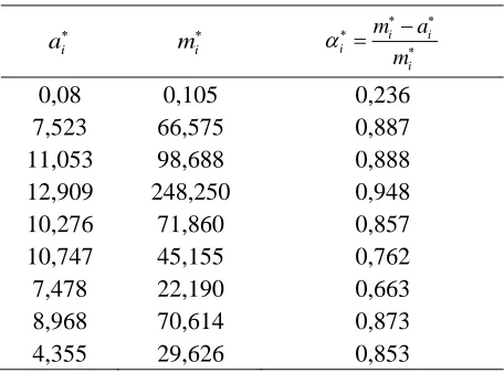
After running the GA-optimization program developed by the recent GA solver of Matlab software, we got the following result of the optimization problem (30):

Table 1: Optimal cession rate by Genetic Algorithms.

i

a m_i i i

i i

m a

m

  



 

0,08 0,105 0,236

7,523 66,575 0,887

11,053 98,688 0,888

12,909 248,250 0,948

10,276 71,860 0,857

10,747 45,155 0,762

7,478 22,190 0,663

8,968 70,614 0,873

4,355 29,626 0,853

5. Conclusion

(12)

This method has shown its effectiveness in terms of the results obtained compared with those in the literature, in terms of its simplicity (effective for optimization problems that are difficult to solve algebraically), or at the level of its precision (improved optimization) which acts on the measure of risk and on the technical benefit, both at the same time with regard to achieving the goal of the insurance company such as maximizing technical benefit and minimizing risk.

Acknowledgements

The authors would like to thank the Journal editorial board and the referees for the interest they have shown in our work and for several valuable comments.

References

1. Aase (2002). Perspectives of risk sharing, Scandinavian Actuarial Journal, 2. 2. Alex Bellos (2011). Alex au pays des chiffres, Robert Laffont.

3. Amédée and Francois, Algorithmes génétiques, TE de fin d’année Tutorat de Mr Philippe Audebaud.

4. Andreani and al (2007). On augmented Lagrangian methods with general lower-level constraint. SIAM Journal on Optimization, 18, 1286–1302.

5. Arrow (1963). Uncertainty and the welfare economics of medical care, American Economic Review.

6. Artzner (1999). Application of coherent risk measures to capital requirements in insurance, North American Actuarial Journal, Vol 3, N° 2.

7. Ben Dbabis (2013). Modèles et méthodes actuarielles pour l’évaluation quantitative des risques en environnement Solvabilité II, Thèse de doctorat, Université Paris Dauphine.

8. Birgin and al (2005). Numerical comparison of augmented Lagrangian algorithms for nonconvex problems, Computational Optimization and Applications, 31. 9. Blazenko (1985). Optimal insurance policies, Insurance: Mathematics and

Economics, Vol 4.

10. Borch (1960). An attempt to determine the optimum amount of stop loss reinsurance, Transactions of the 16th International Congress of Actuaries, 597-610.

11. Boudreault (2010). Mathématiques du risque, Document de référence, Département de mathématiques, Université du Québec à Montréal.

12. Cai and Tan (2007). Optimal Retention for a Stop-Loss Reinsurance Under the VaR and CTE Risk Measures, Astin Bulletin.

13. Davis (1991). The genetic Algorithm Handbook, Ed. New- York: Van Nostrand Reinhold, ch.17.

14. De Finetti (1940). Il problema dei pieni, Giorn. Ist. Ital. Attuari, Vol 1. 15. Deestra and Plantin (2004). La réassurance, Economica.

16. Denault (2001). Coherent Allocation of Risk Capital, Journal of Risk 4, 1-34. 17. Denuit (2004). Charpentier, Mathématiques de l’assurance non vie, tome 1 :

(13)

18. Dickson and Waters (1996). Reinsurance and Ruin, Insurance: Mathematics and Economics, Vol 19.

19. Emiliano and Valdez (2004). Tail Conditional Expectations for Exponential Dispersion Models, University of New South Wales, Sydney, AUSTRALIA . 20. Gajeck and Zagrodny (2000). Insurer’s optimal reinsurance strategies, Insurance :

Mathematics and Economics, Vol. 27.

21. Glineur and Walhin (2004). de Finetti’s Retention Problem for Proportional Reinsurance Revisited, Unpublished manuscript.

22. Goldberg (1989). Genetic Algorithms in search, optimization and Machine learning, Addison-Wesley.

23. Hess (2000). Méthodes actuarielles de l’assurance vie, Economica.

24. Kaas and al (2001). Modern Actuarial Risk Theory, Boston, Dordrecht, London, Kluwer Academic Publishers 28.

25. Kaluszka (2001). Optimal reinsurance under mean-variance premium principles, Insurance: Mathematics and Economics 28, 61-67.

26. Krvavych (2005). Insurer Risk Management and Optimal Reinsurance, PhD Thesis, The University Of New South Wales.

27. Lampaert and Walhin (2005). On the Optimality of Proportional Reinsurance, Casualty Actuarial Society Forum, Spring.

28. Lutton (1999). Algorithmes génétiques et Fractales, Dossier d'habilitation à diriger des recherches, Université Paris XI Orsay.

29. Maling (2013). Optimisation d’un portefeuille de réassurance non-vie : L’exemple du Property and Casualty, Institut de Science Financière et d’Assurances.

30. Moffet (1979). The risk sharing problem, Geneva Papers on Risk and Insurance, 4, 5-13.

31. Mossin (1968). Aspects of rational insurance purchasing, Journal of Political Econ-omy, Vol 79.

32. Ohlin (1969). A generalization of a result by Borch and Kahn on the optimal properties of stop-loss reinsurance, The ASTIN Bulletin, Vol 5.

33. Raviv (1979). The design of an optimal insurance policy, American Economic Review, Vol 69.

34. Renders (1995). Algorithmes génétiques et Réseaux de Neurones, Editions HERMES.

35. Smith (1968). Optimal insurance coverage, Journal of Political Economy, Vol 76. 36. Tan and al (2011). Optimality of general reinsurance contracts under CTE risk

measure, Insurance: Mathematics and Economics, 49(2), 175–187.

37. Tan and Chi (2011). Optimal reinsurance under VaR and CVaR risk measures: A simplified approach, ASTIN Bulletin, 41(2), 487-509.