Bayesian Inference for Double Seasonal Moving Average Models: A Gibbs Sampling Approach

Bayesian Inference for Double Seasonal Moving Average Models:

A Gibbs Sampling Approach

Ayman A Amin

Department of Statistics, Mathematics, and Insurance Faculty of Commerce, Menoufia University, Egypt [email protected]

Abstract

In this paper we use the Gibbs sampling algorithm to develop a Bayesian inference for multiplicative double seasonal moving average (DSMA) models. Assuming the model errors are normally distributed and using natural conjugate priors, we show that the conditional posterior distribution of the model parameters and variance are multivariate normal and inverse gamma respectively, and then we apply the Gibbs sampling to approximate empirically the marginal posterior distributions. The proposed Bayesian methodology is evaluated using simulation study.

Keywords: Bayesian analysis, Double seasonality, Gibbs sampler, Multiplicative seasonal moving average.

1. Introduction

High frequency time series that are observed at small time units may be characterized by exhibiting multiple seasonal patterns. For example, hourly electricity load data can exhibit intraday and intraweek seasonal patterns. Other examples of high frequency time series contain multiple seasonal patterns include daily hospital admissions, daily usage of water and natural gas, hourly volumes of call center arrivals, hourly traffic on a road, hourly access to computer web sites, and half-hourly demand for public transportation. The notion of modelling multiple seasonalities is not new and it can be traced back to 1971 when Thompson and Tiao (1971) showed that monthly disconnections of the Wisconsin telephone company have annual and quarterly (double) seasonal patterns. Accordingly, seasonal autoregressive moving average (SARMA) models being widely applied to analyze time series with single seasonal pattern need to be modified and extended to accommodate multiple seasonalities, see for example Box et al. (1994) and Taylor (2003). In addition to SARMA models, other techniques have been extended to fit multiple seasonal time series, which include neural networks, exponential smoothing methods and innovation state models. A quick review of these techniques can be found in Feinberg & Genethliou (2005).

Other references may include Taylor (2008a&b), Caiado (2008), Baek (2010), Mohamed et al. (2010), Au et al. (2011), Mohamed et al. (2011) and Kim (2013).

Bayesian analysis of SARMA model for single seasonality has been well established, and different approaches have been developed in literature. Analytical approximation is one of these approaches, which simply approximates the posterior and predictive densities to be standard closed-form distributions that are analytically tractable, see for example Shaarawy and Ismail (1987). However, this approach is conditioning on the initial values leading to waste observations, and treats SARMA model as an additive not a multiplicative model which can introduce new unnecessary coefficients in the model. To address the limitations of analytical approximation, in recent years MCMC methods, especially Gibbs sampling algorithm, have been proposed to ease the Bayesian time series analysis. Ismail (2003a&b) used Gibbs sampling algorithm to achieve Bayesian analysis for multiplicative seasonal moving average (SMA) and seasonal autoregressive (SAR) models. This work was extended by Ismail and Amin (2014) to multiplicative SARMA model. The literature in Bayesian analysis of DSARMA models is still immature. Amin and Ismail (2015) have used Gibbs sampling algorithm to develop a Bayesian analysis to multiplicative double SAR models. In the current paper, we extend this work to develop a Bayesian analysis to multiplicative DSMA models based on Gibbs sampling algorithm. The initial idea of this work was presented in the 60th ISI World Statistics Congress 2015, and the main advantages of the proposed methodology are that the Bayesian analysis is unconditional on the initial values of errors and it treats DSMA model as a multiplicative not an additive model to achieve parsimonious property.

The remainder of this paper is organized as follows: Section 2 presents multiplicative DSMA models. Section 3 summarizes the posterior analysis and full conditional posterior distributions of the parameters. The implementation details of the proposed algorithm including convergence monitoring are presented in Section 4. The proposed methodology is illustrated in Section 5 using several simulated examples. Finally, the conclusions are given in Section 6.

2. Double Seasonal Moving Average (DSMA) Model

A time series {𝑦_𝑡} is said to be generated by a multiplicative seasonal moving average model of orders q, Q₁, and Q₂, denoted by DSMA(q)(Q₁)_𝑠1(Q₂)_𝑠2, if it satisfies

𝑦𝑡= 𝜃𝑞(𝐵)Θ𝑄1(𝐵

𝑠1_)Ψ

𝑄2(𝐵

𝑠2_)𝜀

𝑡 (1)

where {𝜀_𝑡} is a sequence of independent normal variates with zero mean and variance 𝜎2. The backshift operator B is defined as 𝐵𝑘𝑦𝑡= 𝑦𝑡−𝑘, s1 and s2 are the seasonal periods. The non seasonal moving average polynomial is 𝜃𝑞(𝐵) = (1 + 𝜃1𝐵 + 𝜃2𝐵2+ ⋯ +

𝜃_𝑞𝐵𝑞_{) with order q. In addition, the seasonal moving average polynomials are}

Θ_𝑄1(𝐵𝑠1_{) = (1 + Θ}

1𝐵𝑠1 + Θ2𝐵2𝑠1+ ⋯ + Θ𝑄1𝐵

𝑄1𝑠1_{) with order Q}

1 and Ψ𝑄2(𝐵

𝑠2_{) =}

(1 + Ψ₁𝐵𝑠2_{+ Ψ}

2𝐵2𝑠2+ ⋯ + Ψ𝑄2𝐵

𝑄2𝑠2_{) with order Q}

2. Finally, the non seasonal and seasonal moving average coefficients are 𝜃 = (𝜃₁, 𝜃₂, ⋯ , 𝜃_𝑞)𝑇, Θ = (Θ₁, Θ₂, ⋯ , Θ_𝑄1)𝑇

It should be noted that the DSMA model (1) has an extra terms compared with the usual multiplicative single SMA model. The new term is Ψ_𝑄2(𝐵𝑠2_{) that accommodates the}

second seasonal pattern. Accordingly, the model (1) can be written as

𝑦_𝑡= ∑ 𝑞 𝑖=1 𝜃_𝑖𝜀_𝑡−𝑖+ ∑ 𝑄1 𝑗=1

Θ_𝑗𝜀_{𝑡−𝑗𝑠1}+ ∑

𝑄2

𝜏=1

Ψ_𝜏𝜀_{𝑡−𝜏𝑠2} + ∑

𝑞

𝑖=1

∑

𝑄1

𝑗=1

𝜃_𝑖Θ_𝑗𝜀_{𝑡−𝑖−𝑗𝑠1}

+ ∑ 𝑞 𝑖=1 ∑ 𝑄2 𝜏=1

𝜃𝑖Ψ𝜏𝜀𝑡−𝑖−𝜏𝑠2 +

∑ 𝑄1 𝑗=1 ∑ 𝑄2 𝜏=1

Θ_𝑗Ψ_𝜏𝜀_{𝑡−𝑗𝑠1−𝜏𝑠2} + ∑

𝑞 𝑖=1 ∑ 𝑄1 𝑗=1 ∑ 𝑄2 𝜏=1

𝜃_𝑖Θ_𝑗Ψ_𝜏𝜀_{𝑡−𝑖−𝑗𝑠1−𝜏𝑠2} + 𝜀_𝑡

= Λ_𝑡𝛽 + 𝜀_𝑡 (2)

where

Λ_𝑡= (𝜀_𝑡−1, … , 𝜀_𝑡−𝑞, 𝜀_𝑡−𝑠1, 𝜀_{𝑡−𝑠1−1}, … , 𝜀_{𝑡−𝑠1−𝑞}, … … , 𝜀_{𝑡−𝑄1𝑠1}, 𝜀_{𝑡−𝑄1𝑠1−1}, … , 𝜀_{𝑡−𝑄1𝑠1−𝑞}, 𝜀_𝑡−𝑠2, 𝜀_{𝑡−𝑠2−1}, … , 𝜀_{𝑡−𝑠2−𝑞}, 𝜀_{𝑡−𝑠1−𝑠2}, 𝜀_{𝑡−𝑠1−𝑠2−1}, … , 𝜀_{𝑡−𝑠1−𝑠2−𝑞}, … … , 𝜀_{𝑡−𝑄1𝑠1−𝑠2}, 𝜀_{𝑡−𝑄1𝑠1−𝑠2−1},

… , 𝜀_{𝑡−𝑄1𝑠1−𝑠2−𝑞}, … … … , 𝜀_{𝑡−𝑄2𝑠2}, 𝜀_{𝑡−𝑄2𝑠2−1}, … , 𝜀_{𝑡−𝑄2𝑠2−𝑞}, 𝜀_{𝑡−𝑠1−𝑄2𝑠2}, 𝜀_{𝑡−𝑠1−𝑄2𝑠2−1}, …,

𝜀𝑡−𝑠1−𝑄2𝑠2−𝑞, … … , 𝜀𝑡−𝑄1𝑠1−𝑄2𝑠2, 𝜀𝑡−𝑄1𝑠1−𝑄2𝑠2−1, … , 𝜀𝑡−𝑄1𝑠1−𝑄2𝑠2−𝑞),

𝛽 = (𝜃1, … , 𝜃𝑞, Θ1, 𝜃1Θ1, … , 𝜃𝑞Θ1, … … , Θ𝑄1, 𝜃1Θ𝑄1, … , 𝜃𝑞Θ𝑄1, Ψ1, 𝜃1Ψ1, … , 𝜃𝑞Ψ1, Θ1Ψ1,

𝜃1Θ1Ψ1, … , 𝜃𝑞Θ1Ψ1, … … , Θ𝑄1Ψ1, 𝜃1Θ𝑄1Ψ1, … , 𝜃𝑞Θ𝑄1Ψ1, … … … , Ψ𝑄2, 𝜃1Ψ𝑄2, …,

𝜃_𝑞Ψ_𝑄2, Θ₁Ψ_𝑄2, 𝜃₁Θ₁Π_𝑄2, … , 𝜃_𝑞Θ₁Ψ_𝑄2, … … , Θ_𝑄1Ψ_𝑄2, 𝜃₁Θ_𝑄1Ψ_𝑄2, … , 𝜃_𝑞Θ_𝑄1Ψ_𝑄2)𝑇. (3) Equation (2) shows that the multiplicative DSMA model can be written as a moving average model of order (1 + 𝑞)(1 + 𝑄1)(1 + 𝑄2) − 1 with some coefficients are products of nonseasonal and seasonal coefficients. Therefore, the DSMA model is nonlinear in the coefficients 𝜃, Θ, and Ψ which complicates its Bayesian analysis. In the following sections we explain how to apply the Gibbs sampling to facilitate the analysis. The DSMA model (2) is invertible if the roots of the polynomials 𝜃_𝑞(𝐵), Θ_𝑄1(𝐵𝑠1_{) and}

Ψ𝑄2(𝐵

𝑠2_{) lie outside the unit circle. For more details about the properties of SARMA}

models see Box et al. (1994).

3. Posterior Analysis

3.1 Likelihood Function

Suppose 𝑦 = (𝑦₁, 𝑦₂, ⋯ , 𝑦_𝑛) is a realization of the DSMA model (2), knowing that 𝜀_𝑡 ~

N(0,𝜎2_{) and employing a straightforward random variable transformation from 𝜀}

𝑡 to 𝑦𝑡, the likelihood function is given by

𝐿(𝜃, Θ, Ψ, 𝜎2_{, 𝜀}

0|𝑦) ∝ (𝜎2)−

𝑛

2exp {− 1

2𝜎2∑

𝑛

where the errors 𝜀_𝑡 is computed directly from the model (2). It is obvious that this likelihood function is a complicated function in 𝜃, Θ, Ψ and 𝜀₀. However, the errors 𝜀_𝑡

can be estimated recursively as follows

𝑒_𝑡 = 𝑦_𝑡− ∑𝑞_𝑖=1𝜃̂_𝑖𝑒_𝑡−𝑖− ∑𝑄1

𝑗=1 Θ̂𝑗𝑒𝑡−𝑗𝑠1 − ∑

𝑄2

𝜏=1 Ψ̂𝜏𝜀𝑡−𝜏𝑠2 − ∑

𝑞 𝑖=1 ∑

𝑄1

𝑗=1 𝜃̂𝑖Θ̂𝑗𝑒𝑡−𝑖−𝑗𝑠1−

∑𝑞_𝑖=1∑𝑄2

𝜏=1 𝜃̂𝑖Ψ̂𝜏𝑒𝑡−𝑖−𝜏𝑠2 − ∑

𝑄1

𝑗=1 ∑ 𝑄2

𝜏=1 Θ̂𝑗Ψ̂𝜏𝑒𝑡−𝑗𝑠1−𝜏𝑠2−

∑𝑞_𝑖=1∑𝑄1

𝑗=1 ∑ 𝑄2

𝜏=1𝜃̂𝑖Θ̂𝑗Ψ̂𝜏𝑒𝑡−𝑖−𝑗𝑠1−𝜏𝑠2 (5)

where 𝜃̂_𝑖 ∈ 𝑅𝑞_{, Θ̂}

𝑗 ∈ 𝑅𝑄1, and Ψ̂𝜏 ∈ 𝑅𝑄2 are consistent estimates obtained by the nonlinear least square (NLS) estimation method. Substituting the estimated errors in the likelihood function (3) results in an approximate likelihood function:

𝐿∗(𝜃, Θ, Ψ, 𝜎2, 𝜀0|𝑦) ∝ (𝜎2)−

𝑛

2exp {− 1

2𝜎2∑ 𝑛

𝑡=1

𝜀_𝑡∗2}

= (𝜎2)−

𝑛

2exp {− 1

2𝜎2(𝑦 − Λ̂𝛽)

𝑇

(𝑦 − Λ̂𝛽)}. (6)

where, 𝛽 is defined in (3), and Λ̂ is a n × ((1 + 𝑞)(1 + 𝑄₁)(1 + 𝑄₂) − 1) matrix with the

𝑡𝑡ℎ row:

Λ̂𝑡= (𝑒𝑡−1, … , 𝑒𝑡−𝑞, 𝑒𝑡−𝑠1, 𝑒𝑡−𝑠1−1, … , 𝑒𝑡−𝑠1−𝑞, … … , 𝑒𝑡−𝑄1𝑠1, 𝑒𝑡−𝑄1𝑠1−1, … , 𝑒𝑡−𝑄1𝑠1−𝑞, 𝑒𝑡−𝑠2,

𝑒_{𝑡−𝑠2−1}, … , 𝑒_{𝑡−𝑠2−𝑞}, 𝑒_{𝑡−𝑠1−𝑠2}, 𝑒_{𝑡−𝑠1−𝑠2−1}, … , 𝑒_{𝑡−𝑠1−𝑠2−𝑞}, … … , 𝑒_{𝑡−𝑄1𝑠1−𝑠2}, 𝑒_{𝑡−𝑄1𝑠1−𝑠2−1},

… , 𝑒𝑡−𝑄1𝑠1−𝑠2−𝑞, … … … , 𝑒𝑡−𝑄2𝑠2, 𝑒𝑡−𝑄2𝑠2−1, … , 𝑒𝑡−𝑄2𝑠2−𝑞, 𝑒𝑡−𝑠1−𝑄2𝑠2, 𝑒𝑡−𝑠1−𝑄2𝑠2−1, …,

𝑒𝑡−𝑠1−𝑄2𝑠2−𝑞, … … , 𝑒𝑡−𝑄1𝑠1−𝑄2𝑠2, 𝑒𝑡−𝑄1𝑠1−𝑄2𝑠2−1, … , 𝑒𝑡−𝑄1𝑠1−𝑄2𝑠2−𝑞). (7)

3.2 Prior Specification

Assuming that the parameters 𝜃, Θ, Ψ and 𝜀0 are independent apriori, given the error variance parameter 𝜎2, the joint prior distribution is

𝜁(𝜃, Θ, Ψ, 𝜎2, 𝜀0) = 𝜁(𝜃|𝜎2)×𝜁(Θ|𝜎2)×𝜁(Ψ|𝜎2)×𝜁(𝜀0|𝜎2)×𝜁(𝜎2)

= 𝑁𝑞(𝜇𝜃, 𝜎2Σ𝜃)×𝑁𝑄1(𝜇Θ, 𝜎

2_Σ

Θ)×𝑁𝑄2(𝜇Ψ, 𝜎

2_Σ

Ψ)×𝑁𝑞∗(𝜇𝜀0, 𝜎

2_Σ

𝜀0)×𝐼𝐺(

𝜈 2,

𝜆 2), (8)

where 𝑞∗_{= 𝑞 + 𝑄}

1𝑠1+ 𝑄2𝑠2, 𝑁𝑟(𝜇, Δ) is the r-variate normal distribution with mean 𝜇 and variance Δ, and IG(a, b) is the inverse gamma distribution with parameters a and b. Therefore, the joint prior distribution can be written as follows

𝜁(𝜃, Θ, Ψ, 𝜎2, 𝜀0) ∝ (𝜎2)−(

𝜈∗

2+1)exp {− 1

2𝜎2[𝜆 + (𝜃 − 𝜇𝜃)𝑇Σ𝜃−1(𝜃 − 𝜇𝜃)

+(Θ − 𝜇Θ)𝑇ΣΘ−1(Θ − 𝜇Θ) + (Ψ − 𝜇Ψ)𝑇ΣΨ−1(Ψ − 𝜇Ψ) +(𝜀0− 𝜇𝜀₀) 𝑇

Σ𝜀−1₀(𝜀0− 𝜇𝜀₀)]}, (9) where

𝜈∗ = 𝜈 + 2𝑞 + 𝑄₁(1 + 𝑠₁) + 𝑄₂(1 + 𝑠₂). (10)

(9) by the approximate likelihood function (6) results in the joint posterior

𝜁(𝜃, Θ, Ψ, 𝜎2, 𝜀₀|𝑦) which may be written as

𝜁(𝜃, Θ, Ψ, 𝜎2_{, 𝜀}

0|𝑦) ∝ (𝜎2)−(

𝑛+𝜈∗

2 +1)exp {− 1

2𝜎2[𝜆 + (𝜃 − 𝜇𝜃)𝑇Σ𝜃−1(𝜃 − 𝜇𝜃)

+ (Θ − 𝜇_Θ)𝑇_Σ

Θ−1(Θ − 𝜇Θ) + (Ψ − 𝜇Ψ)𝑇ΣΨ−1(Ψ − 𝜇Ψ)

+ (𝜀₀− 𝜇_𝜀0)𝑇Σ_𝜀−1_0(𝜀

0− 𝜇𝜀0) + (𝑦 − Λ̂𝛽)

𝑇

(𝑦 − Λ̂𝛽)]} (11)

3.3 Full Conditional Posterior Distributions

The conditional posterior distribution for each one of the DSMA parameters is obtained from the joint posterior distribution (11) by first grouping together terms in the joint posterior that depend on this parameter, and then finding the appropriate normalizing constant to form a proper and closed-form density. In this study all the conditional posteriors obtained for the unknown parameters are normal and inverse gamma distributions for which sampling techniques exist.

3.3.1 The conditional posterior of 𝜽

We obtained the conditional posterior of 𝜃 by finding out 𝜁(𝜃|𝑦, Θ, Ψ, 𝜎2, 𝜀₀) that we proved to be a multivariate normal 𝑁(𝜇_𝜃∗, 𝑣_𝜃∗) with

𝜇_𝜃∗ = [(𝐻_𝜃𝑇𝐻_𝜃+ Σ_𝜃−1)−1(Σ_𝜃−1𝜇_𝜃 + 𝐻_𝜃𝑇(𝑦 − 𝐿𝜃𝛽𝜃))]

and

𝑣_𝜃∗ = 𝜎2_(𝐻

𝜃𝑇𝐻𝜃+ Σ𝜃−1) −1

.

Where, H_𝜃 is a (n × q) matrix with the 𝑡𝑖𝑡ℎ _element:

𝐻𝜃𝑡𝑖 = (𝑒𝑡−𝑖+ ∑

𝑄1

𝑗=1

Θ𝑗𝑒𝑡−𝑖−𝑗𝑠1 + ∑

𝑄2

𝜏=1

Ψ𝜏𝑒𝑡−𝑖−𝜏𝑠2 + ∑

𝑄1

𝑗=1

∑

𝑄2

𝜏=1

Θ𝑗Ψ𝜏𝑒𝑡−𝑖−𝑗𝑠1−𝜏𝑠2),

L_𝜃 is a n × ((1 + 𝑄1)(1 + 𝑄2) − 1) matrix with the 𝑡𝑡ℎ row:

𝐿𝜃𝑡= (𝑒𝑡−𝑠1, … , 𝑒𝑡−𝑄1𝑠1, 𝑒𝑡−𝑠2, 𝑒𝑡−𝑠1−𝑠2, … , 𝑒𝑡−𝑄1𝑠1−𝑠2, … … , 𝑒𝑡−𝑄2𝑠2, 𝑒𝑡−𝑠1−𝑄2𝑠2, … , 𝑒𝑡−𝑄1𝑠1−𝑄2𝑠2),

and 𝛽𝜃 is a column vector of order (1 + 𝑄1)(1 + 𝑄2) − 1 written as:

𝛽𝜃 = (Θ1, … , Θ𝑄1, Ψ1, Θ1Ψ1, … , Θ𝑄1Ψ1, … … , Ψ𝑄2, Θ1Ψ𝑄2, … , Θ𝑄1Ψ𝑄2)

𝑇

.

3.3.2 The conditional posterior of 𝚯

We obtained the conditional posterior of Θ by finding out 𝜁(Θ|𝑦, 𝜃, Ψ, 𝜎2_{, 𝜀}

0) that we proved to be a multivariate normal 𝑁(𝜇_Θ∗, 𝑣_Θ∗) with

𝜇_Θ∗ = [(𝐻_Θ𝑇𝐻_Θ+ Σ_Θ−1)−1_(Σ

Θ−1𝜇Θ+ 𝐻Θ𝑇(𝑦 − 𝐿Θ𝛽Θ))]

and

𝑣_Θ∗ = 𝜎2_(𝐻

Where H_Θ is a (n × Q₁) matrix with the 𝑡𝑗𝑡ℎ element:

𝐻_Θ𝑡𝑗 = (𝑒_{𝑡−𝑗𝑠1}+ ∑

𝑞

𝑖=1

𝜃_𝑖𝑒_{𝑡−𝑖−𝑗𝑠1}+ ∑

𝑄2

𝜏=1

Ψ_𝜏𝑒_{𝑡−𝑗𝑠1−𝜏𝑠2}+ ∑

𝑞

𝑖=1

∑

𝑄2

𝜏=1

𝜃_𝑖Ψ_𝜏𝑒_{𝑡−𝑖−𝑗𝑠1−𝜏𝑠2}),

L_Θ is a n × ((1 + 𝑞)(1 + 𝑄₂) − 1) matrix with the 𝑡𝑡ℎ row:

𝐿_Θ𝑡 = (𝑒_𝑡−1, … , 𝑒_𝑡−𝑞, 𝑒_𝑡−𝑠2, 𝑒_{𝑡−1−𝑠2}, … , 𝑒_{𝑡−𝑞−𝑠2}, … … , 𝑒_{𝑡−𝑄2𝑠2}, 𝑒_{𝑡−1−𝑄2𝑠2}, … , 𝑒_{𝑡−𝑞−𝑄2𝑠2}),

and 𝛽_Θ is a column vector of order (1 + 𝑞)(1 + 𝑄₂) − 1 written as:

𝛽_Θ = (𝜃₁, … , 𝜃_𝑞, Ψ₁, 𝜃₁Ψ₁, … , 𝜃_𝑞Ψ₁, … … , Ψ_𝑄2, 𝜃₁Ψ_𝑄2, … , 𝜃_𝑞Ψ_𝑄2)𝑇.

3.3.3 The conditional posterior of 𝚿

We obtained the conditional posterior of Ψ by finding out 𝜁(Ψ|𝑦, 𝜃, Θ, 𝜎2, 𝜀0) that we proved to be a multivariate normal 𝑁(𝜇_Ψ∗ , 𝑣_Ψ∗) with

𝜇_Ψ∗ = [(𝐻_Ψ𝑇𝐻Ψ+ ΣΨ−1)−1(ΣΨ−1𝜇Ψ+ 𝐻Ψ𝑇(𝑦 − 𝐿Ψ𝛽Ψ))] and

𝑣_Ψ∗ = 𝜎2(𝐻_Ψ𝑇_𝐻

Ψ+ ΣΨ−1)−1.

Where H_Ψ is a (n × Q₂) matrix with the 𝑡𝜏𝑡ℎ element:

𝐻_Ψ𝑡𝜏 = (𝑒_{𝑡−𝜏𝑠2}+ ∑

𝑞

𝑖=1

𝜃_𝑖𝑒_{𝑡−𝑖−𝜏𝑠2}+ ∑

𝑄1

𝑗=1

Θ_𝑗𝑒_{𝑡−𝑗𝑠1−𝜏𝑠2} + ∑

𝑞

𝑖=1

∑

𝑄1

𝑗=1

𝜃_𝑖Θ_𝑗𝑒_{𝑡−𝑖−𝑗𝑠1−𝜏𝑠2}),

L_Ψ is a n × ((1 + 𝑞)(1 + 𝑄₁) − 1) matrix with the 𝑡𝑡ℎ _row:

𝐿_Ψ𝑡 = (𝑒_𝑡−1, … , 𝑒_𝑡−𝑞, 𝑒_𝑡−𝑠1, 𝑒_{𝑡−1−𝑠1}, … , 𝑒_{𝑡−𝑞−𝑠1}, … … , 𝑒_{𝑡−𝑄1𝑠1}, 𝑒_{𝑡−1−𝑄1𝑠1}, … , 𝑒_{𝑡−𝑞−𝑄1𝑠1}),

and 𝛽Ψ is a column vector of order (1 + 𝑞)(1 + 𝑄1) − 1 written as:

𝛽_Ψ = (𝜃₁, … , 𝜃_𝑞, Θ₁, 𝜃₁Θ₁, … , 𝜃_𝑞Θ₁, … … , Θ_𝑄1, 𝜃₁Θ_𝑄1, … , 𝜃_𝑞Θ_𝑄1)𝑇.

3.3.4 The conditional posterior of 𝝈𝟐

We obtained the conditional posterior of 𝜎2 by finding out 𝜁(𝜎2|𝑦, 𝜃, Θ, Ψ, 𝜀0) that we proved to be an inverse gamma 𝐼𝐺(𝑛+𝜈å

2 ,

𝜆+𝑛(𝑆2)

2 ), where 𝜈

∗ _{is defined in (10) and}

𝑛(𝑆2_{) = [(𝜃 − 𝜇}

𝜃)𝑇Σ𝜃−1(𝜃 − 𝜇𝜃) + (Θ − 𝜇Θ)𝑇ΣΘ−1(Θ − 𝜇Θ) + (Ψ − 𝜇Ψ)𝑇ΣΨ−1(Ψ − 𝜇Ψ) +

(𝜀₀− 𝜇_𝜀0)𝑇Σ_𝜀−1_{0 (𝜀}

0− 𝜇𝜀0) + (𝑦 − Λ̂𝛽)

𝑇

(𝑦 − Λ̂𝛽)].

To ease the Gibbs sampling algorithm process, the parameter 𝜎2 can be sampled from the Chi square distribution using the transformation 𝜆+𝑛(𝑆

2₎

(𝜎2₎ ~𝜒(𝑛+𝜈2 ∗).

3.3.5 The conditional posterior of 𝜺_𝟎

In the beginning, we write explicitly the elements of 𝜀₀ using the model (2) as follows:

𝑦_𝑞∗ = 𝑀𝜀₀+ 𝑁𝜀_𝑞∗, (12)

𝑀 =

(

𝛼₁ 𝛼₂ 𝛼₃ ⋯ ⋯ 𝛼_𝑞∗₋₁ 𝛼_𝑞∗

𝛼₂ 𝛼₃ 𝛼₄ ⋯ ⋯ 𝛼_𝑞∗ 0

𝛼₃ 𝛼₄ ⋯ ⋯ 0 0

⋮ ⋮ ⋮ ⋯ ⋯ ⋮ ⋮

𝛼_𝑝∗₋₁ 𝛼_𝑝∗ 0 ⋯ ⋯ 0 0

𝛼_𝑝∗ 0 0 ⋯ ⋯ 0 0

)_(𝑞∗_)×(𝑞∗₎

,

𝑁 =

(

1 0 0 ⋯ ⋯ 0 0

𝛼1 1 0 ⋯ ⋯ 0 0

𝛼₂ 𝛼₁ 1 ⋯ ⋯ 0 0

⋮ ⋮ ⋮ ⋯ ⋯ ⋮ ⋮

𝛼𝑝∗−1 𝛼𝑝∗−2 ⋯ ⋯ 𝛼2 𝛼1 1

)_(𝑞∗_)×(𝑞∗₎

,

𝑞∗ = 𝑞 + 𝑄1𝑠1+ 𝑄2𝑠2 and 𝜀𝑝∗ = (𝜀1, 𝜀2, … 𝜀𝑞∗) 𝑇

that has the 𝑞∗ multivariate normal distribution with zero mean and variance (𝜎2𝐼_𝑞∗), where 𝐼_𝑞∗ is the unit matrix of order 𝑞∗.

Using the above defined matrices and the standard Bayesian techniques, we obtained the conditional posterior of 𝜀0 by finding out 𝜁(𝜀0|𝑦, 𝜃, Θ, Ψ, 𝜎2) that we proved to be a multivariate normal 𝑁(𝜇𝜀0

∗ _{, 𝑣} 𝜀0

∗ _{) with}

𝜇_𝜀∗₀ = [𝐻_𝜀0𝑀 + Σ_𝜀−1₀ ]−1[Σ_𝜀−1₀ 𝜇_𝜀0 + 𝐻_𝜀0𝑦_𝑞∗]

and

𝑣𝜀0

∗ _{= 𝜎}2_[𝐻

𝜀0𝑀 + Σ𝜀0

−1_]−1_,

where, 𝐻_𝜀0 = 𝑀𝑇_(𝑁𝑁𝑇₎−1_.

4. The Proposed Gibbs Sampler

The proposed Gibbs sampling algorithm for DSMA model can be implemented as follows:

1. Specify starting values 𝜃0_{, Θ}0_{, Ψ}0_{, (𝜎}2₎0 _{and 𝜀}

00 and set j=0. A set of initial estimates of

the model parameters can be obtained using the NLS method.

2. Calculate the residuals recursively using (5) and the NLS estimates.

3. Simulate

• 𝜃𝑗~𝜁(𝜃𝑗|𝑦, (𝜎2)𝑗−1, Θ𝑗−1, Ψ𝑗−1, 𝜀0𝑗−1),

• Θ𝑗_~𝜁(𝜃𝑗_{|𝑦, (𝜎}2₎𝑗−1_{, 𝜙}𝑗_{, Ψ}𝑗−1_{, 𝜀} 0𝑗−1),

• Ψ𝑗_~𝜁(Ψ𝑗_{|𝑦, (𝜎}2₎𝑗−1_{, 𝜃}𝑗_{, Θ}𝑗_{, 𝜀} 0𝑗−1),

• (𝜎2)𝑗~𝜁((𝜎2)𝑗|𝑦, 𝜃𝑗, Θ𝑗, Ψ𝑗, 𝜀0𝑗−1),

• 𝜀0𝑗~𝜁(𝜀0𝑗|𝑦, (𝜎2)𝑗, 𝜃𝑗, Θ𝑗, Ψ𝑗),

This algorithm gives the next value of the Markov chain

{𝜃𝑗+1_{, Θ}𝑗+1_{, Ψ}𝑗+1_{, (𝜎}2₎𝑗+1_{, 𝜀} 0 𝑗+1

} by simulating each of the full conditionals where the conditioning elements are revised during the cycle. This iterative process is repeated for a large number of iterations and continuously the convergence is monitored. After the chain has converged, say at 𝑛₀ iterations, the simulated values

{𝜃𝑗+1_{, Θ}𝑗+1_{, Ψ}𝑗+1_{, (𝜎}2₎𝑗+1_{, 𝜀} 0 𝑗+1

} are used as a sample from the joint posterior. Posterior estimates of the parameters are computed directly via sample averages of the simulation outputs. The convergence of the Gibbs sampler’s Markov chain can be monitored by three groups of diagnostics, which include autocorrelation coefficients estimates, Raftery and Lewis diagnostics, and Geweke diagnostics. First, autocorrelation coefficients estimates indicate how much independence exists in the sequence of each parameter draws. High values of autocorrelation coefficients indicate more draws needed to get accurate posterior estimates. Second, diagnostics proposed by Raftery and Lewis (1992,1995) include (1) Burn: number of draws used as initial draws before starting to sample the draws for posterior inference, (2) Nmin: number of draws that would be needed if the draws represented an iid chain, (3) Total: total number of draws needed to achieve desired level of accuracy, and (4) I-stat: the ratio of the (Total) to (Nmin). Raftery and Lewis suggested that a convergence problem is indicated when values of I-stat exceed 5. Third, diagnostics proosed by Geweke (1992), which includes two groups: 1. The first group includes the relative numerical efficiency (RNE) and numerical standard errors (NSE). The RNE estimates indicate the required number of draws to produce the same numerical accuracy when iid sample is drawn directly from the posterior distribution. The NSE estimates reflect the variation that can be expected if the simulation were to be repeated.

2. The second group of diagnostics includes a test of whether the Gibbs sampler has attained an equilibrium state. This can be achieved by testing the equality of the two means of the first and last parts of draws and the Chi squared marginal probability is obtained. Usually, the first and last parts are the first 20% and the last 50% of the draws.

LeSage (1999) implemented these convergence using Matlab package, and we use them in the following section to monitor the convergence of our proposed Gibbs sampling algorithm for DSMA model.

5. Simulation Study

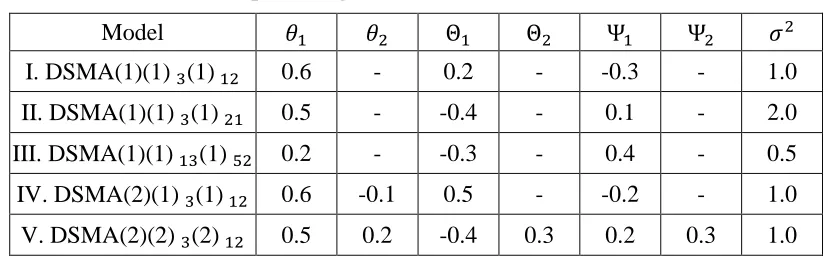
Table 1: Simulated examples design.

Model 𝜃₁ 𝜃₂ Θ₁ Θ₂ Ψ₁ Ψ₂ 𝜎2

I. DSMA(1)(1)₃(1)₁₂ 0.6 - 0.2 - -0.3 - 1.0

II. DSMA(1)(1)₃(1)₂₁ 0.5 - -0.4 - 0.1 - 2.0

III. DSMA(1)(1)₁₃(1)₅₂ 0.2 - -0.3 - 0.4 - 0.5 IV. DSMA(2)(1)₃(1)₁₂ 0.6 -0.1 0.5 - -0.2 - 1.0 V. DSMA(2)(2)₃(2)₁₂ 0.5 0.2 -0.4 0.3 0.2 0.3 1.0

Once the time series datasets of size 𝑛 = 1,000 are generated from these selected DSMA models, the Bayesian analysis is performed by assuming a non informative prior for the parameters 𝜃, Θ, Ψ and 𝜎2 _{and a normal prior with zero mean for initial errors 𝜀}

0 with variance 𝜎2𝐼𝑞∗. To apply the proposed Gibbs sampler, the starting values for the parameters 𝜃, Θ, Ψ and 𝜎2 are obtained using NLS method, and the starting values for 𝜀₀

are assumed to be zeros. For each dataset, the Gibbs sampler was run 11,000 iterations where the first 1,000 draws are ignored and every tenth value in the sequence of the last 10,000 draws is recorded to have an approximately independent sample of 1,000 draws. Accordingly, all posterior estimates of the parameters are computed directly as sample averages of the 1,000 Gibbs sampler draws. In the following, we discuss the results of the proposed algorithm and investigate its convergence.

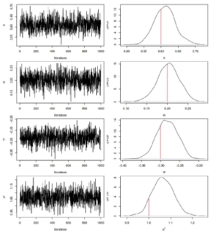
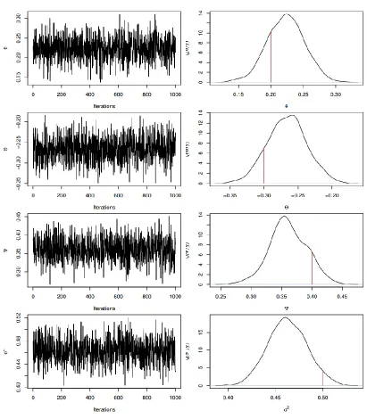
Table 1 presents the true values and the Bayesian estimates of the parameters for example I. In addition, a 95% confidence interval using the 0.025 and 0.975 percentiles of the simulated draws is constructed for every parameter. From Table 1, it is clear that the Bayesian estimates are close to the true values and the 95% confidence interval includes the true value for each parameter. Sequential plots of the parameters generated sequences together with marginal densities are displayed in Figure 1. The marginal densities are computed using non parametric technique with Gaussian kernel. Figure 1 shows that the proposed algorithm is stable and fluctuates in the neighborhood of the true values. In addition, the marginal densities show that the true value of each parameter (which is indicated by the vertical line) falls in the constructed 95% confidence interval.

Table 2: Bayesian results for example I.

Parameter True

Values Mean

Std. Dev.

Lower

95 % limit Median

Upper 95 % limit

𝜃 0.60 0.61 0.03 0.55 0.61 0.67

Θ 0.20 0.20 0.03 0.15 0.20 0.25

Ψ -0.30 -0.28 0.03 -0.33 -0.28 -0.23

Figure 1: Sequential plots and marginal posterior distributions of example I

equal means hypothesis can not be rejected and no dramatic differences between the NSE estimates are found. In addition, the RNE estimates are close to 1 which indicates the iid nature of the output sample.

Table 3: Autocorrelations and Raftery-Lewis diagnostics for example I.

Parameter Autocorrelations Raftery-Lewis Diagnostics

Lag 1 Lag 5 Lag 10 Lag 50 Burn Total(N) (Nmin) I-stat

𝜃 0.03 0.04 0.01 -0.01 3 1117 994 1.12

Θ 0.01 0.03 0.01 -0.04 2 1028 994 1.03

Ψ 0.00 0.00 -0.01 0.01 2 1028 994 1.03

𝜎2 -0.02 -0.00 -0.02 -0.00 2 948 994 0.95

Table 4: Geweke diagnostics for example I.

Parameter NSE iid

RNE iid

NSE 4%

RNE 4%

NSE 8%

RNE 8%

NSE 15%

RNE

15% 𝜒

2

𝜃 0.0009 1 0.0010 0.93 0.0009 1.07 0.0009 1.17 0.98

Θ 0.0008 1 0.0006 1.78 0.0005 2.31 0.0005 2.99 0.96

Ψ 0.0008 1 0.0008 1.05 0.0008 1.15 0.0007 1.27 0.83

𝜎2 0.0015 1 0.0014 1.11 0.0012 1.50 0.0011 2.00 0.63

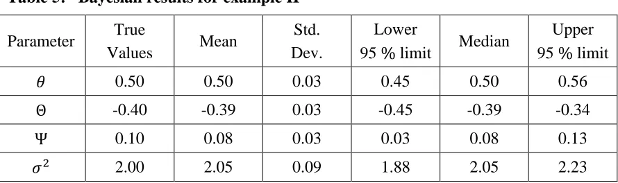
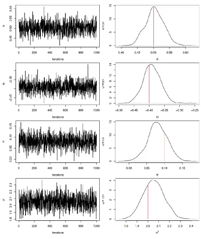
Similarly to example I, Tables 4-7 present the true values and Bayesian estimates of the parameters for examples II - V. In addition, sequential plots with marginal densities of these examples are displayed in Figures 2 - 5. Similar conclusions to those of example I are obtained. We have applied the proposed Gibbs sampler to several simulated datasets from other DSMA models; and we found their results are similar to those of presented examples, and therefore they are not presented here.

Table 5: Bayesian results for example II

Parameter True

Values Mean

Std. Dev.

Lower

95 % limit Median

Upper 95 % limit

𝜃 0.50 0.50 0.03 0.45 0.50 0.56

Θ -0.40 -0.39 0.03 -0.45 -0.39 -0.34

Ψ 0.10 0.08 0.03 0.03 0.08 0.13

Figure 2: Sequential plots and marginal posterior distributions of example II

Table 6: Bayesian results for example III

Parameter True

Values Mean

Std. Dev.

Lower

95 % limit Median

Upper 95 % limit

𝜃 0.20 0.22 0.03 0.17 0.22 0.28

Θ -0.30 -0.27 0.03 -0.32 -0.27 -0.21

Ψ 0.40 0.36 0.03 0.30 0.36 0.42

Figure 3: Sequential plots and marginal posterior distributions of example III

Table 7: Bayesian results for example IV.

Parameter True

Values Mean

Std. Dev.

Lower

95 % limit Median

Upper 95 % limit

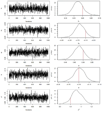
𝜃₁ 0.60 0.57 0.03 0.52 0.57 0.64

𝜃₂ -0.10 -0.14 0.03 -0.19 -0.14 -0.08

Θ 0.50 0.48 0.03 0.42 0.48 0.53

Ψ -0.20 -0.20 0.02 -0.25 -0.20 -0.15

Figure 4: Sequential plots and marginal posterior distributions of example IV

Table 8: Bayesian results for example V

Parameter True

Values Mean

Std. Dev.

Lower

95 % limit Median

Upper 95 % limit

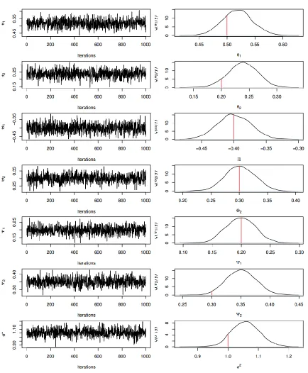
𝜃₁ 0.50 0.52 0.03 0.47 0.52 0.57

𝜃₂ 0.20 0.24 0.03 0.19 0.24 0.29

Θ₁ -0.40 -0.40 0.02 -0.45 -0.40 -0.35

Θ2 0.30 0.30 0.03 0.25 0.30 0.35

Ψ₁ 0.20 0.20 0.02 0.15 0.20 0.25

Ψ₂ 0.30 0.35 0.03 0.30 0.35 0.40

Figure 5: Sequential plots and marginal posterior distributions of example V

6. Conclusion

approximate empirically the marginal posterior distributions along with using several diagnostics that showed the convergence of the proposed algorithm was achieved. Accordingly, we computed directly the posterior estimates of the parameters via sample averages of the simulation outputs. The simulation results confirmed the accuracy of the proposed methodology. Future work may investigate model identification using stochastic search variable selection, outliers detection, and extension to multivariate double seasonal models.

References

1. Amin, A.A. and Ismail, M.A. (2015). Gibbs Sampling for Double Seasonal Autoregressive Models. Communications for Statistical Applications and Methods, 22(6), 557-573.

2. Au, T, Ma, G.Q, and Yeung, SN (2011). Automatic Forecasting of Double Seasonal Time Series with Applications on Mobility Network Traffic Prediction. 2011 Joint Statistical Meetings, July 30-August4, Miami Beach, Florida, USA. 3. Baek, M. (2010). Forecasting Hourly Electricity Loads of South Korea:

Innovations State Space Modeling Approach. The Korean Journal of Economics 17(2), 301-317.

4. Box, G.E.P, Jenkins, G.M and Reinsel, G.C. (1994). Time Series Analysis: Forecasting and Control, 3rd ed, Prentice-Hall, Inc.:NJ.

5. Caiado, J (2008). Forecasting Water Consumption in Spain Using Univariate Time Series Models. MPRA Paper no. 6610.

6. Cortez, P., Rio, M., Rocha, M. and Sousa, P. (2012). Multi-scale Internet Traffic Forecasting Using Neural Networks and Time Series Methods. Expert Systems 29 (2), 143-155.

7. Cruz, A., Munoz,A., Zamora, J.L., Espinola, R. (2011). The effect of Wind Generation and Weekday on Spanish Electricity Spot price Forecasting. Electric Power Systems Research 81(10), 1924–1935.

8. Feinberg, E. and Genethliou, D. (2005). Load forecasting. In F. W. J. Chow, Applied Mathematics for Restructured Electirc Power Systems: Control and Computational Intelligence (pp. 269-285). Springer.

9. Geweke, J. (1992). Evaluating the Accuracy of Sampling-Based Approaches to the Calculations of Posterior Moments. In Bayesian Statistics 4, J. M., Bernardo, J. O., Berger, A. P., Dawid, and A. F. M., Smith, (eds), 641-649. Oxford, Clarendon Press.

10. Ismail, M. A. (2003a). Bayesian Analysis of Seasonal Autoregressive Models. Journal of Applied Statistical science, 12(2), 123-136.

11. Ismail, M. A. (2003b). Bayesian Analysis of Seasonal Moving Average Model: A Gibbs Sampling Approach. Japanese Journal of Applied Statistics, 32(2), 61-75. 12. Ismail, M.A. and Amin, A.A. (2014). Gibbs Sampling for SARMA Models.

13. LeSage, J. P. (1999). Applied Econometrics using Matlab. Dept. of Economics, University of Toledo, available at http://www.econ.utoledo.edu.

14. Raftrey, A. E. and Lewis, S. (1992). One long run with diagnostics: Implementation strategies for Markov Chain Monte Carlo. Statistical Science, 7, 493-497.

15. Raftrey, A. E. and Lewis, S. (1995). The number of iterations, convergence diagnostics and generic Metropolis algorithms. In Practical Markov Chain Monte

Carlo, W. R., Gilks, D. J., Spiegelhalter and S., Richardson, (eds). London,

Chapman and Hall.

16. Shaarawy, S. and Ismail, M. A. (1987). Bayesian Inference for Seasonal ARMA Models. The Egyptian Statistical Journal, 31, 323-336.

17. Kim, M.S. (2013). Modeling Special-day Effects for Forecasting Intraday Electricity demand, European Journal of Operational Research 230(1), 170-180. 18. Mohamed, N., Ahmad, M.H., Ismail, Z. and Suhartono (2010). Double Seasonal

ARIMA Model for Forecasting Load Demand. Matematika 26 (2), 217-231. 19. Mohamed, N, Ahmad, MH and Suhartono (2011). Forecasting Short Term

Demand Using Double Seasonal ARIMA Model. World Applied Sciences Journal 13, 27-35.

20. Taylor, J.W. (2003). Short-Term Electricity Demand Forecasting Using Double Seasonal Exponential Smoothing. The Journal of the Operational Research Society 54(8), 799-805.

21. Taylor, J. W., de Menezes, L. M. and McSharry, P. A (2006). Comparison of Univariate Methods for Forecasting Electricity Demand up to a Day ahead. International Journal of Forecasting 22: 1–16.

22. Taylor, J. W. (2008a). An Evaluation of Methods for very Short-term Load Forecasting using Minute-by-Minute British Data. International Journal of Forecasting 24: 645– 658.

23. Taylor, J.W. (2008b). A Comparison of Univariate Time Series Methods for Forecasting Intraday Arrivals at a Call Center. Management Science 54, 253-265. 24. Thompson, H.E, and Tiao, G.C. (1971). Analysis of Telephone Data. The Bell