MSEPBurr Distribution: Properties and Parameter Estimation

MSEPBurr Distribution: Properties and Parameter Estimation

Achmad Syahrul Choir

Doctoral Student at Department of Statistics

Faculty of Mathematics, Computation, and Science Data Institut Teknologi Sepuluh Nopember, Surabaya, Indonesia BPS-Statistics Indonesia

[email protected]

Nur Iriawan

Department of Statistics

Faculty of Mathematics, Computation and Science Data Institut Teknologi Sepuluh Nopember, Surabaya, Indonesia [email protected]

Brodjol Sutijo Suprih Ulama

Department of Business Statistics, Faculty of Vocational Institut Teknologi Sepuluh Nopember, Surabaya, Indonesia [email protected]

Mohammad Dokhi

Politeknik Statistika STIS, Jakarta, Indonesia [email protected]

Abstract

MSNBurr and MSTBurr distribution have been developed as Neo-Normal distributions that represent a relaxation of normality. The difference between them is that the MSTBurr’s peak is below MSNBurr’s. In this paper, we propose a MSEPBurr distribution with its peak could be not only lower but also high-er than MSNBurr. Furthermore, we study several properties of MSEPBurr, such as mean, variance, skewness, kurtosis, and quantile. The MSEPBurr parameters are estimated by using the Bayesian approach with the BUGS language implementation for its computation. We employ simulation study and use existing data to illustrate the application of the regression model. In real data, we notice that MSEPBurr has similar performance with MSNBurr and MSTBurr that they outperform Normal and Student-t distribution in Australian athlete data because their skewness can accommodate long left tail excellently. However, their performance is less than the Student-t model in chemical reaction rate data because their skewness can not accommodate long right tail perfectly. Although in general their perfor-mance is the same, we observe that the MSEPBurr performs better than the MSNBurr and the MSTBurr in some simulated data.

Keywords: Distribution, Bayesian, Normal Relaxation, MSEPBurr, MSNBurr, MSTBurr

1. Introduction

distribution. This distribution has symmetrical or skewed properties with an unstable mode at its location parameter. An extended Skew-Normal distribution has been applied to regression analysis by Olosunde Akinlolu (2011). In contrast to Azzalini (1985), Fernandez and Steel (1998) proposed the Skew-Normal distribution that has a stable mode of the location parameter. The study of the skewed or symmetrical distribution has been carried out by Iriawan (2000) who developed the “Modified to be Stable as Normal from Burr”, hereinafter referred to MSNBurr distribution. It was derived from the modification of Burr type II distribution (Burr, 1942). The mode of MSNBurr distribution is stable like that of the Skew-Normal distribution (Fernandez and Steel, 1998). The symmetrical MSNBurr perfectly fits the Normal distribution, but its tails are fatter than that of the Normal distribution.

Iriawan (2000) also developed the “Modified to be Stable as t from Burr”, hereinafter referred to MSTBurr distribution with its peak could be below MSNBurr’s when their location and scale parameters are the same. In this paper, we propose “Modified to be Stable Exponential Power from Burr”, henceforth referred to MSEPBurr distribution with its peak could be not only lower but also higher than MSNBurr distribution.

2. The Neo-Normal Distribution

The Neo-Normal distribution is a distribution, which represents a relaxation of the Normal distribution (Iriawan, 2000). This distribution can be the same or different from the Normal distribution due to the shape parameter that plays a role in assigning the magnitude of kurtosis or skewness. One of the preliminary works of relaxation of the Normal distribution was conducted by Box and Tiao (1973) who investigate EP distribution. The probability density function (pdf) of a random variable 𝑍₁ that follows EP distribution is

𝑓(𝑧₁|𝜇, 𝜎, 𝑣) =𝐶(𝑣)

𝜎 𝑒𝑥𝑝 (−𝑞(𝑣) |

𝑧1− 𝜇

𝜎 |

2/(1+𝑣)

), (1)

where −∞< 𝑧₁ < ∞, −∞< 𝜇 <∞, 𝜎 > 0, −1 < 𝑣 < 1,

𝑞(𝑣) = (𝛤 (

3

2(1 + 𝑣))

𝛤 (1₂(1 + 𝑣))) 1/(1+𝑣)

, 𝐶(𝑣) = 𝛤 (

3

2(1 + 𝑣))

1 2

(1 + 𝑣)𝛤 (1₂(1 + 𝑣))

3 2

.

The height of the mode of the EP distribution could be higher or lower than the Normal distribution, depending on the value of parameter 𝑣. _{The Normal distribution is a special form} of EP distribution when 𝑣 = 0.

Iriawan (2000) has developed the Neo-Normal distribution from modified Burr type II distribution (Burr, 1942). The Burr type II distribution is also known as Generalized Logistic type I (Johnson et al., 1995; Abdelfattah, 2015). The cumulative distribution function (CDF) and pdf of a random variable 𝑍₂ that follows the Burr type II distribution are given by

𝐹(𝑧₂) = (1 + 𝑒𝑥𝑝( − 𝑧₂))−𝛼_,

(2)

and

𝑓(𝑧₂|𝛼) = 𝛼 𝑒𝑥𝑝( − 𝑧₂)(1 + 𝑒𝑥𝑝( − 𝑧₂))−(𝛼+1)_,

respectively, where −∞< 𝑧₂ < ∞, and 𝛼 > 0. _{The mode of Burr type II distribution is varied} according to the value of parameter 𝛼. Iriawan (2000) modified Equation (2) by transforming 𝑍3 = 𝑍2− 𝑙𝑜𝑔 𝛼 so that its CDF became as follows

𝐹(𝑧₃) = (1 +𝑒𝑥𝑝( − 𝑧3)

𝛼 )

−𝛼

, (4)

and the corresponding pdf in Equation (3) became

𝑓(𝑧₃|𝛼) = 𝑒𝑥𝑝( − 𝑧₃) (1 +𝑒𝑥𝑝( − 𝑧3)

𝛼 )

−(𝛼+1)

. (5)

The distribution with CDF in the Equation (4) and pdf in Equation (5) was called the “Modified Stable Burr” or 𝑀𝑆𝐵𝑢𝑟𝑟(𝛼). The mode of the MSBurr would be stable at 𝑧₃ = 0for any value of the parameter 𝛼. Similar to Burr type II distribution, howe-ver, the density of its mode always lower than that of the Standard Normal distribu-tion. For comparison with 𝑁𝑜𝑟𝑚𝑎𝑙(𝜇, 𝜎2), Iriawan (2000), therefore, added a parameter 𝜔 and defined a transformation as follows

𝑍₄ = 𝜇̃ + 𝜎̃ 𝜔𝑍3. The CDF in Equation (4) would be as follows:

𝐹(𝑧4) = (1 +

𝑒𝑥𝑝( − 𝜔 (𝑧4−𝜇̃

𝜎 ̃ ))

𝛼 )

−𝛼

, (6)

and its pdf in Equation (5) is transformed into: 𝑓(𝑧4|𝜔, 𝛼, 𝜇̃, 𝜎̃)

= 𝜔

𝜎̃𝑒𝑥𝑝 (−𝜔 (

𝑧₄− 𝜇̃

𝜎̃ )) (1

+𝑒𝑥𝑝 (−𝜔 (

𝑧4−𝜇̃

𝜎 ̃ ))

𝛼 )

−(𝛼+1)

,

(7)

where −∞< 𝑧₄ <∞,−~,𝜎̃ > 0, 𝛼 > 0.

As described above, Iriawan (2000) has derived MSBurr distribution from modified Burr type II distribution, such that its mode is stable at its location parameter 𝜇 either it is symmetric or skewed. Further, the MSBurr distribution could be modified, in such that its peak as high as certain symmetric unimodal distribution. The step for the last modification is described in the Theorem 1.

Theorem 1. Making the density of MSBurr’s mode the same as the density of other symmetrical unimodal distributions’ mode

Suppose 𝑍₄ follows 𝑀𝑆𝐵𝑢𝑟𝑟(𝜔, 𝛼, 𝜇̃, 𝜎̃) and 𝑍∗ follows a symmetric uni-modal distribution with pdf as

ℎ(𝑧∗_|𝜇∗_{, 𝜎}∗_{, 𝜃}∗_{) = 𝑔 (}𝑧∗− 𝜇∗ 𝜎∗ |𝜃∗),

i.ℎ(𝜇∗|𝜎∗, 𝜃∗) =_𝐶̃(𝜃1_∗)𝜎∗, where 𝐶̃(𝜃∗) is the function of shape parameter that is a normalizing constant of g,

ii. 𝜎̃ = 𝜎∗, and

iii. 𝑓(𝜇̃|𝜔, 𝛼, 𝜎̃) = ℎ(𝜇∗|𝜎∗, 𝜃∗), where f(.) is pdf of MSBurr distribution, then

𝜔 =(1 +

1 𝛼)

(𝛼+1)

𝐶̃(𝜃∗₎ .

Proof:

Suppose 𝑍₄~𝑀𝑆𝐵𝑢𝑟𝑟(𝜔, 𝛼, 𝜇̃, 𝜎̃), _{so pdf of} 𝑍₄ on its location parameter 𝜇̃ follows

𝑓(𝜇̃|𝜔, 𝛼, 𝜎̃) =𝜔

𝜎̃𝑒𝑥𝑝 (−𝜔 (

𝜇̃ − 𝜇̃

𝜎̃ )) (1 +

𝑒𝑥𝑝 (−𝜔 (𝜇̃−𝜇_𝜎̃̃))

𝛼 )

−(𝛼+1)

,

=𝜔 𝜎̃(1 +

1 𝛼)

−(𝛼+1) . Given the mode of 𝑍₄ is equal to 𝑍∗,

𝑓(𝜇̃|𝜔, 𝛼, 𝜎̃) = ℎ(𝜇∗_|𝜎∗_{, 𝜃}∗_),

𝜔 𝜎̃(1 +

1 𝛼)

−(𝛼+1)

= 1

𝐶̃(𝜃∗_)𝜎∗. If 𝜎̃ = 𝜎∗, then we get

𝜔 =(1 + 1 𝛼)

(𝛼+1)

𝐶̃(𝜃∗₎ .

Corollary 1. MSNBurr distribution

The density of 𝑀𝑆𝐵𝑢𝑟𝑟(𝜔, 𝛼, 𝜇̃, 𝜎̃) on its mode will be equal to the density of 𝑁𝑜𝑟𝑚𝑎𝑙(𝜇̃, 𝜎̃)’s mode when

𝜔 =(1 + 1 𝛼)

(𝛼+1)

√2𝜋 .

(8)

Corollary 2. MSTBurr distribution

The density of 𝑀𝑆𝐵𝑢𝑟𝑟(𝜔, 𝛼, 𝜇̃, 𝜎̃) on its mode will be equal to the density of 𝑡(𝜇̃, 𝜎̃, 𝑣̈)′𝑠 mode when

𝜔 =𝛤 ( 𝑣̈+1

2 ) (1 +

1 𝛼)

(𝛼+1)

√𝑣̈𝜋𝛤 (𝑣̈₂) .

(9)

“Modified to be Stable to t from Burr” or MSTBurr(𝑣̈, 𝛼, 𝜇̃, 𝜎̃) _when 𝜔 satisfies Equation (9) (Iriawan, 2000).

Following Corollary 1 and Corollary 2, the new modified MSBurr distribution with its peak as high as the mode of EP distribution is proposed. Equation (1) showed that the normalizing constant has a function of shape parameter as follows

𝐶̃(𝑣) =(1 + 𝑣)𝛤 ( 1

2(𝑣 + 1))

3 2

𝛤 (3₂(𝑣 + 1))

1 2

.

By employing Theorem 1, MSBurr’s peak would be as high as EP’s when

𝜔 =𝛤 ( 3

2(𝑣 + 1))

1

2_{(1 +}1

𝛼) (𝛼+1)

(1 + 𝑣)𝛤 (1₂(𝑣 + 1))

3 2

. (10)

Figure 1. The comparison of MSEPBurr(0,1,0,1), MSEPBurr(-0.9,1,0,1), MSEPBurr (0.9,1,0,1), and MSNBurr(1,0,1)

The MSBurr distribution with 𝜔 satisfies Equation (10) is referred to as the MSEP-Burr distribution. Because it was derived from EP distribution, it is natural if its peak could be either lower or higher than that of MSNBurr distribution when their location and scale parameters are the same. The comparison of MSEPBurr distribution and MSNBurr distribution was shown in Figure 1. This figure shows that MSEPBurr distribution close to MSNBurr distribution when 𝑣 = 0.

3. Properties of MSEPBurr Distribution

𝐾𝑍4(𝑡) = 𝑡𝜇̃ −

𝜎̃𝑡

𝜔 𝑙𝑜𝑔 𝛼 + 𝑙𝑜𝑔 𝛤 (𝛼 +

𝜎̃𝑡

𝜔) + 𝑙𝑜𝑔 𝛤 (1 −

𝜎̃𝑡

𝜔)

− 𝑙𝑜𝑔 𝛤 (𝛼).

(11)

The first moment of 𝑀𝑆𝐵𝑢𝑟𝑟(𝜔, 𝛼, 𝜇̃, 𝜎̃) deriving from the first cumulant (𝜅₁) is

(

)

~ ~ , ) ( 0 0 1 4         − − + = = Z E (12)

where 𝜓0(. )is digamma function. Furthermore, the r-th central moment deriving from r-th cumulant is

(

)

where 𝜓_(𝑟−1)(. )is an r-th derivative of 𝑙𝑜𝑔 𝛤 (. ), 𝑟 = 2,3, . .. . Based on moment in Equ-ation (12) and central moment in Equation (13) where 𝜔 _{follows Equation (10), the mean} (𝐸(𝑍_4𝑒)), variance (𝑉𝑎𝑟(𝑍_4𝑒)), skewness (𝛾₁(𝑍_4𝑒)),and excess kurtosis (𝛾₂(𝑍_4𝑒))of 𝑍_4𝑒 which follows the MSEPBurr distribution is defined as

𝐸(𝑍_4𝑒) = 𝜇̃ + 𝜎̃(1 + 𝑣)𝛤 (

1

2(𝑣 + 1))

3 2

𝛤 (3₂(𝑣 + 1))

1 2

(1 +1_𝛼)(𝛼+1)

(𝜓₀(𝛼) − 𝜓₀(1) − 𝑙𝑜𝑔 𝛼), (14)

𝑉𝑎𝑟(𝑍4𝑒) =

𝜎̃2_{(1 + 𝑣)𝛤 (}1

2(𝑣 + 1)) 3

𝛤 (3₂(𝑣 + 1)) (1 +_𝛼1)2(𝛼+1)

(𝜓1(𝛼) + 𝜓1(1)), (15)

𝛾1(𝑍4𝑒) =

(𝜓₂(𝛼) − 𝜓₂(1)) (𝜓1(𝛼) + 𝜓1(1))

3 2

, (16)

𝛾₂(𝑍_4𝑒) = (𝜓3(𝛼) + 𝜓3(1)) (𝜓1(𝛼) + 𝜓1(1))2,

(17)

Figure 2. Plot of skewness of MSEPBurr where 0.1 ≤ 𝛼 < 10

It is easy to see that 𝛼 is a parameter which has a role in determining the magnitude of the skewness and kurtosis. Figure2 shows that MSEPBurr distribution is symme-tric when 𝛼 = 1. Otherwise, this distribution is left skew if 𝛼 < 1, and is right skew if 𝛼 > 1. It is shown that the magnitude of negative skewness is greater than positive skewness. It means that the MSEPBurr distribution more adaptively accommodate the left skew data than right skew one, in particular when 𝛼 < 1. Moreover, Figure 3 shows that the minimum value of excess kurtosis in MSEPBurr distribution is 1.2, which is when 𝛼 = 1. This shows that the MSEPBurr distribution is leptokurtic. The kurtosis is influenced by the value of skewness. The left skew MSEPBurr distribution has a sharper peak than the right skew one.

Figure 3. Plot of MSEPBurr’s excess kurtosis

Another property discussed in this paper is the quantile of the MSEPBurr distribution. We obtain the quantile by using inverse of CDF in Equation (6), where 𝜔 follows Equation (10), that leads to

𝑄(𝑢) = 𝜇̃ − 𝜎̃(1 + 𝑣)𝛤 (

1

2(𝑣 + 1))

3 2

𝛤 (3₂(𝑣 + 1))

1

2_{(1 +}1

𝛼)

(𝛼+1)(𝑙𝑜𝑔 𝛼 + 𝑙𝑜𝑔 (𝑢

−_𝛼1 _{− 1))}

(18)

Based on the Equation (18), the random numbers that have MSEPBurr distribution could be drawn by using the invers transform as in Algorithm 1.

Algorithm 1. Generating the MSEPBurr random number

Step 1.Generate 𝑢~𝑈(0,1),

Step 2.Calculate 𝑧4𝑒 = 𝑄(𝑢) from Equation (18), Step 3.Return 𝑧_4𝑒 (as MSEPBurr random number).

4. Parameter Estimation of MSEPBurr Using Bayesian

1.2

We estimate the MSEPBurr distribution parameters using the Bayesian approach. The parameter estimator is obtained from the posterior distribution, which is proportional to the likelihood times the prior distribution. Let 𝑍4𝑖 follows the MSEPBurr(𝑣, 𝛼,𝜇̃, 𝜎̃) distribution, i=1, 2, ...,n, where n is the sample size, then the likelihood of the MSEPBurr distribution is

𝑓(𝒛𝟒𝒆|𝑣, 𝛼, 𝜇̃, 𝜎̃) = ∏

𝛤 (3₂(𝑣 + 1))

1 2

(1 +_𝛼1)(𝛼+1)

𝜎̃(1 + 𝑣)𝛤 (1₂(𝑣 + 1))

3 2

𝐸𝑖

(1 +𝐸𝑖

𝛼) (𝛼+1) 𝑛 𝑖=1 , = 𝛤 ( 3

2(𝑣 + 1))

𝑛

2_{(1 +}1

𝛼) 𝑛(𝛼+1)

𝜎̃𝑛_{(1 + 𝑣)}𝑛_{𝛤 (}1

2(𝑣 + 1))

3𝑛 2

∏ 𝐸𝑖

(1 +𝐸𝑖

𝛼) (𝛼+1) 𝑛 𝑖=1 , (19)

where 𝒛_𝟒𝒆= (𝑧_4𝑒1, 𝑧_4𝑒2, . . . , 𝑧_4𝑒𝑛)𝑇, and

𝐸_𝑖 = 𝑒𝑥𝑝

(

𝛤 (3₂(𝑣 + 1))

1 2

(1 +_𝛼1)(𝛼+1)

(1 + 𝑣)𝛤 (1₂(𝑣 + 1))

3 2

(𝑧4𝑒𝑖− 𝜇̃

𝜎̃ )

) .

In this research, the prior distributions for the MSEPBurr parameters are set to:

a. 𝛼~𝐺𝑆𝐵𝑒𝑡𝑎(𝑞∗, 𝑙𝑏, 𝑢𝑏), 0 < 𝑙𝑏 < 𝑢𝑏<∞,

where GSBeta or Generalized Symmetrical Beta is a Beta distribution wich its domain is widened in the interval 𝑙𝑏 < 𝛼 < 𝑢𝑏, and it has pdf as

𝑓(𝛼) =𝛤(2𝑞

∗_{)((𝛼 − 𝑙}

𝑏)(𝑢𝑏− 𝛼))(𝑞

∗₋₁₎

𝛤(𝑞∗₎2_(𝑢

𝑏− 𝑙𝑏)(2𝑞∗−1) ,

(20)

where 𝑞∗ ≥ 1 (Box and Tiao, 1973),

b. 𝑣~𝐺𝑆𝐵𝑒𝑡𝑎(𝑞𝑣∗, 𝑙𝑏𝑣, 𝑢𝑏𝑣), −1 < 𝑙𝑏𝑣 < 𝑢𝑏𝑣 < 1, where its pdf is 𝑓(𝑣) = 𝛤(2𝑞𝑣∗)((𝑣 − 𝑙𝑏𝑣)(𝑢𝑏𝑣− 𝑣))(𝑞𝑣

∗₋₁₎

𝛤(𝑞𝑣∗)2(𝑢𝑏𝑣− 𝑙𝑏𝑣)(2𝑞𝑣∗−1) ,

(21)

where 𝑞_𝑣∗ ≥ 1

c. 𝜇̃~𝑁𝑜𝑟𝑚𝑎𝑙(𝜐₀, 𝜑₀2) where its pdf is

𝑓(𝜇̃) = 1

𝜑0√2𝜋

𝑒𝑥𝑝 (−1

2

(𝜇̃ − 𝜐₀)2 𝜑₀2

0

) (22)

d. 𝜎̃~𝐼𝑛𝑣𝑒𝑟𝑠𝑒 − 𝑔𝑎𝑚𝑚𝑎(𝑎0, 𝑏0) where its pdf is

𝑓(𝜎̃) = 𝑏0

𝑎0

𝛤(𝑎₀)𝜎̃(−𝑎0−1)𝑒𝑥𝑝 (− 𝑏₀

𝜎̃). (23)

The joint posterior distribution of MSEPBurr parameters, obtained by multiplying the likelihood in Equation (19) and the independent prior distributions in Equation (20) to Equation (23), is defined as follows

𝑓(𝑣, 𝛼, 𝜇̃, 𝜎̃|𝒛𝟒𝒆) ∝ 𝑓(𝒛𝟒𝒆|𝑣, 𝛼, 𝜇̃, 𝜎̃)𝑓(𝑣)𝑓(𝛼)𝑓(𝜇̃)𝑓(𝜎̃). ₍₂₄₎

a. 𝑓(𝑣|𝐳𝟒𝒆, 𝛼, 𝜇̃, 𝜎̃) ∝

𝛤 (3₂(𝑣 + 1))

𝑛 2

(1 + 𝑣)𝑛_{𝛤 (}1

2(𝑣 + 1))

3𝑛 2

∏ 𝐸𝑖

(1 +𝐸𝑖

𝛼) (𝛼+1) 𝑛 𝑖=1 × ((𝑣 − 𝑙𝑏𝑣)(𝑢𝑏𝑣− 𝑣))(𝑞𝑣 ∗₋₁₎ (25)

b. 𝑓(𝛼|𝐳_𝟒𝒆, 𝑣, 𝜇̃, 𝜎̃) ∝ (1 +1 𝛼)

𝑛(𝛼+1)

∏ 𝐸𝑖

(1 +𝐸𝑖

𝛼) (𝛼+1) 𝑛 𝑖=1 × ((𝛼 − 𝑙𝑏)(𝑢𝑏− 𝛼))(𝑞 ∗₋₁₎ (26)

c. 𝑓(𝜇̃|𝒛_𝟒𝒆, 𝛼, 𝑣, 𝜎̃) ∝ 𝑒𝑥𝑝 (−1 2

(𝜇̃ − 𝜐0)2

𝜑02 ₀) ∏

𝐸𝑖

(1 +𝐸𝑖

𝛼) (𝛼+1) 𝑛 𝑖=1 (27)

d. 𝑓(𝜎̃|𝒛𝟒𝒆, 𝛼, 𝑣, 𝜇̃) ∝ 𝜎̃−(𝑛+𝑎0+1)𝑒𝑥𝑝 (− 𝑏₀

𝜎̃) . ∏

𝐸_𝑖

(1 +𝐸𝑖

𝛼) (𝛼+1) 𝑛

𝑖=1

(28)

We employ Markov Chain Monte Carlo (MCMC) algorithm, particularly Gibbs Sam-pler algorithm in the computation of the MSEPBurr parameters estimation. This algo-rithm is described in Algorithm 2. Algorithm 2 could be applied into Bayesian In-ference Using Gibbs Sampler (BUGS) language (Lunn et al., 2000), that employs Just Another Gibbs Sampling (JAGS) software (Plummer, 2003). This program is run by the runjags package (Denwood, 2016) in R software (R Core Team, 2017). The MSEPBurr had been added in the runjags module as a new distribution in JAGS.

Algorithm 2. The Gibbs Sampler algorithm for the MSEPBurr parameter estimation

1. Set the initial value of 𝑣(0), 𝛼(0), . 𝜇̃(0), 𝜎̃(0).

2. For each t-th iteration, where t = 1,2, ..., T, T is number of samples, a. Generate 𝑣(𝑡)from 𝑓(𝑣(𝑡)|𝒛𝟒𝒆, 𝛼(𝑡−1), 𝜇̃(𝑡−1), 𝜎̃(𝑡−1)) in Equation (25),

b. Generate 𝛼(𝑡) from 𝑓(𝛼(𝑡)|𝒛𝟒𝒆, 𝑣(𝑡), 𝜇̃(𝑡−1), 𝜎̃(𝑡−1)) in Equation (26),

c. Generate 𝜇̃(𝑡)from 𝑓(𝜇̃(𝑡)|𝒛𝟒𝒆, 𝛼(𝑡), 𝑣(𝑡), 𝜎̃(𝑡−1)) in Equation (27),

d. Generate 𝜎̃(𝑡) from 𝑓(𝜎̃(𝑡)|𝒛𝟒𝒆, 𝛼(𝑡), 𝑣(𝑡), 𝜇̃(𝑡)) in Equation (28).

3. Return 𝑣(1), . . . , 𝑣(𝑇), 𝛼(1), . . . , 𝛼(𝑇), 𝜇̃(1), . . . , 𝜇̃(𝑇), 𝜎̃(1), . . . , 𝜎̃(𝑇).

The estimators of MSEPBurr parameter are computed from output in Algorithm 2. They are

𝑣̂ =∑ 𝑣(𝑡) 𝑇 𝑡 𝑇 ,𝛼̂ = ∑ 𝛼𝑇𝑡 (𝑡) 𝑇 , , ~ ˆ~ () T T t t



We do a simulation study to investigate the performance of the MSEPBurr distri-bution when it is applied to regression modeling. This simulation is started by ge-nerating data y and x which has a linear relationship as follows

𝑦̃_𝑖 = 𝛽̃₀+ 𝛽̃₁𝑥_𝑖 + 𝜀̃_𝑖, 𝑖 = 1,2, . . . , 𝑛, ₍₂₉₎

where n is the number of observations, 𝛽̃₀ was set to 1, 𝛽̃_{1 was set to 2, and} 𝜀̃_𝑖 follows MSEPBurr(0.8,10,0,1) that represents right-skew data. There are 4 generated numbers of data (n), i.e.: 10, 30, 100, and 1000. Moreover, the generating simulated data is repeated in 10 iterations.

We define 4 regression models for each data simulation. These models are

• Model 1 is a simple linear regression with errors follow the Normal distribution,

• Model 2 is a simple linear regression with errors follow the MSNBurr distribution,

• Model 3 is a simple linear regression with errors follow the MSTBurr distribution,

• Model 4 is a simple linear regression with errors follow the MSEPBurr distribution.

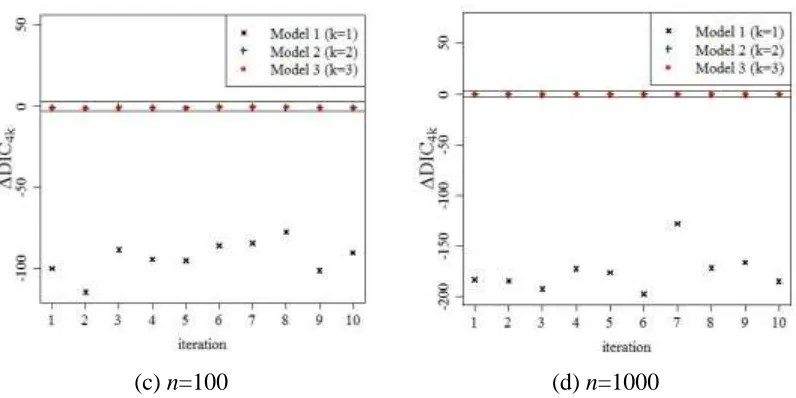
Next, the model parameters in each generated data are estimated by using a Bayesian approach. Each prior of 𝛽̃₀ and 𝛽̃₁ is Normal(0,0.1). In Model 1, the prior of the pre-cision parameter (𝜏) follows Gamma(1,1). The prior of the parameter 𝛼 and 𝜎̃ in Maudel 2, Model 3, and Model 4 follow GSBeta(1,0.1,15) and Inverse-gamma(1,1), respectively. The prior of the shape parameter 𝑣° in Model 3 follows Uniform(1,100). The prior of the shape parameter 𝑣 _{in Model} 4 follows GSBeta(1,-0.99,1). In addi-tion, the performance of each model is compared using its Deviance Information Cri-teria (DIC) (Spiegelhalter et al., 2002; Spiegelhalter et al., 2014). Carlin and Louis (2008) stated that when the DIC differences lies between 3 and 5, usually could be considered the smallest DIC is a better model. The difference between DIC of each model is denoted by

𝛥𝐷𝐼𝐶4𝑘 = 𝐷𝐼𝐶4− 𝐷𝐼𝐶𝑘,

where 𝐷𝐼𝐶4 is DIC of Model 4 and 𝐷𝐼𝐶𝑘 is DIC of Model k, k=1, 2, 3. When |𝛥𝐷𝐼𝐶4𝑘| ≤ 3 then there is no evidence that Model 4 is better than Model k. If 𝛥𝐷𝐼𝐶_4𝑘 > 3, the performance of Model k can be considered better than the Model 4. Otherwise, if 𝛥𝐷𝐼𝐶_4𝑘 < −3, the performance of Model 4 is considered better than Model k.

(c) n=100 (d) n=1000 Figure 4. 𝜟𝑫𝑰𝑪𝟒𝒌where k=1,2,3 in scenario 2 (a) n=10, (b) n=30, (c) n=100, (d) n=1000

The comparison of each model performance based on simulation data is presented in Figure 4. Two horizontal lines in the middle of these figures are created as 𝛥𝐷𝐼𝐶 = 3 and 𝛥𝐷𝐼𝐶₄ = −3, respectively. Figure 4 (a) shows that when n=10, Model 4 outper-forms over other models in 3 of 10 simulation data. However, Figure 4 (b), (c), and (d) shows that Model 4 has the same performance as Model 2 and Model 3. In addi-tion, Figure 4 shows that Model 1 always has the lowest performance because of Nor-mal distribution can not handle asymmetric residuals.

6. Application

In this section, the MSEPBurr regression was applied to two real data sets. The MSEPBurr distribution was compared to Normal, Student-t, MSNBurr, and MSTBurr distribution. In the first example, the regression model was applied using popular “Australian Athletes” data set that has been studied by Rubio and Genton (2016). In the second example, we employ the chemical reaction rate in Box and Tiao (1973) that has been analyzed by Albert et al. (1991). The DIC was used for model performance comparison. The computation of model parameters was also performed using JAGS software that is run using runjags package in R software. The posterior samples of each parameter are obtained by 5,000 burn-in in 255,000 iterations. Moreover, we used 25 thin to reduce autocorrelation in MCMC output. Using the autorun function in this package, the iteration could be automatically added when convergence has not been achieved. Furthermore, the convergence of MCMC was checked using potential scale reduction factor (PSRF) (Gelman and Rubin, 1992; Brooks and Gelman, 1997).

6.1 Australian athletes data

The model for the first data is as follows (Rubio and Genton, 2016)

𝑦_𝑖∗= 𝛽1∗𝑥1𝑖∗ + 𝛽2∗𝑥2𝑖∗ + 𝜀∗𝑖, 𝑖 = 1,2, . . . ,102, (30)

vague prior. The prior distributions of 𝛽₁∗_and 𝛽₂∗ are assigned to 𝑁𝑜𝑟𝑚𝑎𝑙(0,106). The priors of the precision (𝜎−2) _{in the Normal and Student-t distributions were specified to} Gamma(0.001,0.001). The scale parameters (𝜎) in other distributions were set to Inverse-Gamma(0.001,0.001). The prior of degrees of freedom (𝑣_𝑡) in the Student-t model was determined to Uniform(1,50). Other than that, we set the prior of the parameters 𝛼 of MSNBurr, MSTBurr, and MSEPBurr model as GSBeta(1,0,10) and the prior of the parameters 𝑣̈ in MSTBurr model and 𝑣̈ in MSEPBurr model were set to Uniform(1,50) and GSBeta(1,-0.9,1) respectively.

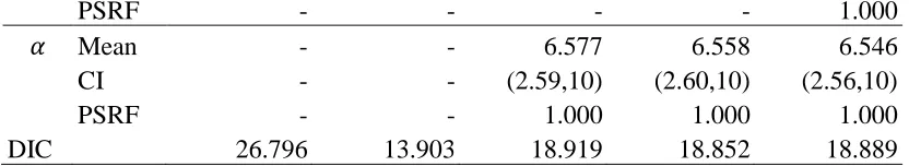
Table 1. Male Australian Athletes Data: Posterior mean, credible interval (CI), PSRF, and DIC

Parameter Errors Distribution

Normal Student-t MSNBurr MSTBurr MSEPBurr

𝛽₁∗ _{Mean 0.077 0.061 0.042 0.042 0.042}

CI (0.06,0.10) (0.04,0.08) (0.02,0.06) (0.02,0.07) (0.02,0.06)

PSRF 1,000 1,000 1.008 1,000 1,004

𝛽₂∗ _{Mean 0.732 0.772 0.826 0.826 0.826}

CI (0.69,0.78) (0.73,0.82) (0.77,0.88) (0.77,0.88) (0.77,0.88)

PSRF 1,000 1.000 1.006 1,000 1,004

𝜎 Mean 2.299 1.259 1.486 1.459 1.600

CI (1.99,2.62) (0.90,1.64) (1.19,1.78) (1.17,1.75) (0.92,2.56)

PSRF 1.000 1.000 1.000 1.000 1.000

Tabel 1. (continued)

𝑣𝑡 Mean - 2.517 - - -

CI - (1.20,4.20) - - -

PSRF - 1.000 - - -

𝑣̈ Mean - - - 25.516-

CI - - - (2.81,49.16) -

PSRF - - - 1.000 -

v Mean - - - - -0.002

CI - - - -

(-0.98,0.90)

PSRF - - - - 1.000

𝛼 Mean - - 0.224 0.224 0.224

CI - - (0.06,0.4) (0.07,0.4) (0.07,0.40)

PSRF - - 1.001 1.000 1.003

DIC 461,979 438,665 430,301 430,769 430,432

have lowest performance. The DIC of the Student-t model show that the Student-t model is better than the Normal model. However, both distributions have higher DIC than those of MSNBurr, MSTBurr and MSEPBurr models, which the last three have almost similar DIC. This result indicates that MSNBurr, MSTBurr and MSEPBurr models are better than Normal and Student-t models to capture the pattern of male Australian athletes’ data into a linear regression model. It is because the skewness parameters of their error distributions (𝛼) are less than one, which cannot be accommodated by Normal and Student-t.

6.2 Chemical reaction rate data

The second data is modeled by the Box and Tiao formula (Box and Tiao, 1973)

𝑦_𝑖 = 𝛽₀+ 𝛽₁𝑥_𝑖 + 𝜀_𝑖, 𝑖 = 1,2, . . . ,20, ₍₃₁₎

where

, log i

i L

y = 𝛽0 = 𝑙𝑜𝑔 𝐴 −𝐸_𝑆𝑇̄−1, ,

000 , 50 1

S E

=

 𝑥𝑖 = (𝑇𝑖−1− 𝑇̄−1) × 50,000,

𝐿_𝑖 = 𝑙𝑜𝑔 𝐴 −𝐸_𝑆𝑇1

𝑖, and 𝑇̄

−1 _{= ∑ 𝑇}

𝑖−1, 20 𝑖=1

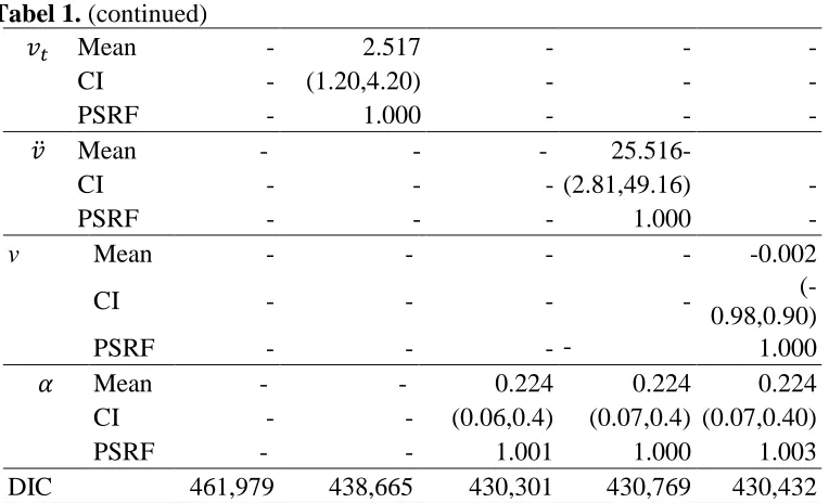
where S is the known gas constant, T is the temperature, and A and E is a constant to be estimated. The errors in this model (𝜀_𝑖) are also assumed following Normal, Student-t, MSNBurr, MSTBurr or MSEPBurr distribution, respectively. We specified prior of these model parameters as vague prior. These priors are the same as the priors in the first example.

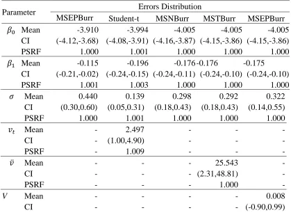
Table 2. Chemical Reaction Data Rate: Posterior mean, credible interval, PSRF, and DIC

Parameter Errors Distribution

MSEPBurr Student-t MSNBurr MSTBurr MSEPBurr

𝛽₀ Mean -3.910 -3.994 -4.005 -4.005 -4.005

CI (-4.12,-3.68) (-4.08,-3.91) (-4.16,-3.87) (-4.15,-3.86) (-4.15,-3.86)

PSRF 1.000 1.001 1.000 1.000 1.000

𝛽₁ Mean -0.115 -0.196 -0.176 -0.176 -0.175 CI (-0.21,-0.02) (-0.24,-0.15) (-0.24,-0.11) (-0.24,-0.10) (-0.24,-0.10)

PSRF 1.001 1.003 1.000 1.000 1.000

𝜎 Mean 0.440 0.139 0.298 0.292 0.322

CI (0.30,0.60) (0.05,0.31) (0.18,0.43) (0.18,0.43) (0.14,0.55)

PSRF 1.000 1.001 1.000 1.000 1.000

𝑣_𝑡 Mean - 2.497 - - -

CI - (1.00,4.90) - - -

PSRF - 1.009 - - -

𝑣̈ Mean - - - 25.543 -

CI - - - (2.31,48.81) -

PSRF - - - 1.000 -

PSRF - - - - 1.000

𝛼 Mean - - 6.577 6.558 6.546

CI - - (2.59,10) (2.60,10) (2.56,10)

PSRF - - 1.000 1.000 1.000

DIC 26.796 13.903 18.919 18.852 18.889

Table 2 shows that the MCMC samples are converging on all parameters because their PSRF value is 1. It also shows that MSNBurr, MSTBurr and MSEPBurr have skewness parameter 𝛼 > 1. This parameter means they have a right-skew residuals. In addition, Student-t model have a degree of freedom 𝑣_𝑡 = 0 which it shows long tail residuals. Based on the DIC value, the Normal model seem have lowest performance in chemical reaction rate data. The MSNBurr, MSTBurr and MSEPBurr models have similar performance and they outperform Normal model. However, their performance is less than the Student-t model because their skewness can not well capture the long right tail.

7. Conclusion

This paper has presented MSEPBurr distribution as a general form of MSNBurr distribution. We also have studied the properties of this distribution. The mean and variance of MSEPBurr are affected by v parameter, but not for the skewness and kurtosis which they are only influenced by the 𝛼 parameter. The simulation study showed that the MSEPBurr has better performance in some data, but in general, the performances of MSEPBurr, MSNBurr, and MSTBurr are almost the same. The MSEPBurr, MSNBurr, and MSTBurr models have similar performance when they are applied to male Australian athletes data and chemical reaction rate data. The MSEPBurr, MSNBurr and MSTBurr models outperform Normal and Student-t models in Australian athletes data because they perfectly accommodate left skew residuals. However, performance of MSEPBurr, MSNBurr and MSTBurr is lower than Stu-dent-t model in chemical reaction rate data because their skewness are not perfectly accommodate long right tail.

Acknowledgements

The first author gratefully acknowledges the support received from BPS-Statistics In-donesia in terms of doctoral scholarship. The authors are grateful to the reviewers for their significant advices to improve this paper. The authors also thank Sarni Maniar Berliana for some comments and corrections.

References

1. Abdelfattah, A. M. (2015). Skew-Type I Generalized Logistic Distribution and its Properties. Pakistan Journal of Statistics and Operation Research, 11(3), 267–282.

3. Azzalini, A. (1985). A Class of Distribution which Includes the Normal Ones. Scandinavian Journal of Statistics, 12(2), 171–178.

4. Box, G. E., and Tiao, G. C. (1973). Bayesian Inference in Statistical Analysis. Reading, Massachusetts: Addison Wesley.

5. Brooks, S. P., and Gelman, A.( 1997). General Methods for Monitoring Convergence of Iterative Simulations. Journal of Computational and Graphical Statistics, 7, 434–455. 6. Burr, I. W. (1942). Cumulative Frequency Functions. The Annals of Mathematical

Statistics, 13(2), 215–232.

7. Carlin, B. P., and Louis, T. A. (2008). Bayesian Methods for Data Analysis (Third ed.). Boca Raton: Chapman and Hall/CRC.

8. Denwood, M. J. (2016). runjags: An R Package Providing Interface Utilities, Model Templates, Parallel Computing Methods and Additional Distributions for MCMC Models in JAGS. Journal of Statistical Software, 71(9), 1–25.

9. Fernandez, C., and Steel, M. (1998). On Bayesian Modelling of Fat Tails and Skewness. Journal of the American Statistical Association, 93(441), 359–371.

10.Gelman, A., and Rubin, D. B. (1992). Inference from Iterative Simulation Using Multiple Sequences. Statistical Science, 7, 457–511.

11.Iriawan, N. (2000). Computationally Intensive Approaches to Inference in Neo-Normal Linear Models. Ph.D. Thesis, CUT-Australia.

12.Johnson, N. L., Kotz, S., and Balakhrisnan, N. (1995). Continuos Univariate Distribution (2 ed., Vol. II ). New York: John Wiley and Son.

13.Lunn, D., Thomas, A., Best, N., and Spiegelhalter, D. (2000). WinBUGS-A Bayesian Modelling Framework: Concepts, Structure, and Extensibility. Statistics and Computing, 10, 325–337.

14.Olosunde Akinlolu,A. (2011). On Skew-Normal Model for Economically Active Population. Pakistan Journal of Statistics and Operation Research, 7(2), 233–243.

15.Plummer, M. (2003). JAGS: A Program for Analysis of Bayesian Graphical Models Using Gibbs Sampling. Proceedings of the 3rd International Workshop on Distributed Statistical Computing (DSC 2003), March 20-22. Vienna, Austria.

16.R Core Team. (2017). R: A Language and Environment for Statistical Computing. Vienna, Austria: R Foundation for Statistical Computing.

17.Rubio, F. J., and Genton, M. G. (2016). Bayesian Linear Regression with Skew-Symmetric Error Distributions with Applications to Survival Analysis. Statistics in Medicine, 35(14), 2441–2454.

18.Spiegelhalter, D. J., Best, N. G., Carlin, B. P., and Van Der Linde, A. (2002). Bayesian measures of model complexity and fit. Journal of the Royal Statistical Society: Series B (Statistical Methodology), 64(4), 583--639.

19.Spiegelhalter, D. J., Best, N. G., Carlin, B. P., and van der Linde, A. (2014). The deviance information criterion: 12 years on. Journal of the Royal Statistical Society: Series B (Statistical Methodology), 76(3), 485–493.