Likelihood Inference for Generalized Integer Autoregressive Time Series Models

Article

Likelihood Inference for Generalized Integer

Autoregressive Time Series Models

Harry Joe

Department of Statistics, University of British Columbia, Vancouver, BC V6T 1Z4, Canada; [email protected]

Received: 17 May 2019; Accepted: 2 October 2019; Published: 11 October 2019

Abstract: For modeling count time series data, one class of models is generalized integer autoregressive of order p based on thinning operators. It is shown how numerical maximum likelihood estimation is possible by inverting the probability generating function of the conditional distribution of an observation given the past p observations. Two data examples are included and show that thinning operators based on compounding can substantially improve the model fit compared with the commonly used binomial thinning operator.

Keywords: count time series; binomial thinning; thinning operators; compounding operation; self-generalized property

1. Introduction

Modeling of count times series has been an active area of research (seeDavis et al. 2015and Weiß 2018) for a few decades. There are applications in business and econometrics, health and medical studies; the models can be applied in general situations for count response variables with time dependence and covariates.

One class of count time series models is based on thinning operators, which are replacements of the multiplication operator to maintain support on the non-negative integers. The theory for count time series modeling with thinning operators has two approaches: (a) models with a specified stationary univariate margin combined with operators that can yield Markov times series models with a lag 1 serial correlation between 0 to 1; (b) models based on thinning operators applied to pprevious observations and a distribution for the innovation, so that in the stationary setting, the autocorrelation functions have similar properties to the Gaussian case (except only positive serial correlations are possible).

The general model of type (b) is generalized integer autoregressive of order p, denoted as GINAR(p). For GINAR(p), mainly the binomial thinning operator has been used, whereas there are many thinning operators proposed for models of type (a).

For models of type (a), there is an extension to include covariates if the distribution of the innovation and the univariate margin are in the same infinitely divisible family, and then the convolution parameter can be a function of covariates. For models of type (b), the extension to include covariates typically requires the parameters of the innovation distribution to be function of the covariates.

For type (a), estimation can usually proceed with numerical maximum likelihood. For type (b), the estimation method is typically method of moments or conditional least squares. The disadvantage of the latter two estimation methods is that the predictive distributions for the next observations given the recent observations cannot be obtained.

In this paper, we use some numerical techniques from the literature for models of type (a) for parameter estimation in GINAR(p) models. The numerical technique applies when there is closed form for the probability generating function (pgf) of the conditional distribution of the next observation

given the past because the pgf can be efficiently numerically inverted to get the conditional probability mass function for likelihood calculations.

The remainder of the paper is organized as follows. Section2describes the background and notation for count times series models and thinning operators. Section3presents the formulation of GINAR(p). Section4presents some probabilistic properties of GINAR(p) in the stationary setting. Section5presents the details to show how the likelihood can be numerically computed, and includes some simulation results. Section6presents two data examples that show how generalized thinning operators lead to better models than binomial thinning. Section7presents the concluding discussion.

2. Background for Thinning Operators

This section presents the background and notation for count data and thinning operators. Let{Yt:t=1, 2, . . .}be a count time series (a sequence of dependent random variables), where Yt ∈ N0 = {0, 1, 2 . . . ,}. The realized data will be denoted as{yt : t = 1, 2, . . . ,n}for a sample of sizen. If there are trend/seasonal terms or covariates at timet, they are incorporated into a vectorxt. We mainly consider the case of small counts, with zeros and overdispersion relative to Poisson.

For early research in Markov count time series with given margins, some references areMcKenzie (1986, 1987), Al-Osh and Aly(1992), Alzaid and Al-Osh (1993). Lettingα denote

the non-negative lag 1 serial correlation, the integer autoregressive model of order 1 has the form:

Yt=Rt(Yt−1;α) +et(α), t=1, 2, . . . , 0≤α≤1. (1)

Ythas a (parametric) distribution such as Poisson, negative binomial (NB) or generalized Poisson. The innovation random variables areet(α)∈ N0fort=1, 2, . . ., and the serially dependent component of the model consists of random variablesRt(y;α)∈ N0such that

E[Rt(Yt−1;α)|Yt−1=y] =E[Rt(y;α)] =αy, y∈ N0, 0≤α≤1, (2)

and Yt=d Rt(Yt−1;α) +et(α) for all 0 ≤ α ≤ 1. Please note that to preserve the space of N0 (non-negative integers), (2) must hold in expectation:Rt(y;α)≡αyis possible only for real-valued or

non-negative reals.

Some examples include the following. (a)Yt∼Poisson andRt(y;α)∼Binomial(y;α)for binomial

thinning; (b)Yt∼negative binomial andRt(y;α)has a beta-binomial distribution; (c)Yt∼generalized

Poisson andRt(y;α)has a quasi-binomial distribution.

For an extension to include covariates, if Yt, Rt(Yt−1;α) and et(α) are in the same

convolution-closed family for all 0<α<1 with a convolution parameterϑ, thenϑcan be a function

of the covariates. However, with this approach, the extension to Markov of higher order is not simple. Markov of order 2 is tractable, but not order 3 or more; seeJoe(1996) and Section 8.4.4 ofJoe(1997).

A broad class of generalized thinning operators with the property of (2) can be obtained with a family of compounding operators based on a family of random variables{K(α): 0≤α≤1}, where

K(α)∈ N0and E[K(α)] =α.

Definition 1(Compounding operator based on random variableK). Let K be a non-negative integer random variable and let y be a non-negative integer. Then K as a compounding operator is denoted as K~y, where

K~y=d y

∑

Ki

With the family{K(α) : 0 ≤ α ≤ 1} of compounding random variables acting as thinning

operators, in (1) let

Rt(y;α) =

y

∑

Kti(α),

whereKti(α)are independent replicates ofK(α)andK(α)has pgfGK(s;α) =E[sK(α)]for 0≤s≤1.

With the~notation, the Markov stationary count time series model can be written as

Yt=Kt(α)~Yt−1+et(α) =

Yt−1

∑

Kti(α) +et(α), t=1, 2, . . . (3)

For the expectation thinning requirement, α = 0 implies K(α) ≡ 0 and et = Yt in (3) for an independent and identically distributed sequence, andα = 1 impliesK(α) ≡ 1 andet = 0 in (3) for perfect dependence.

Please note that ifK has pgfGKandY has pgfGY, thenK~yhas pgf Gy_KandK~Yhas pgf GY◦GK.

With the family{K(α)}of compounding operators, a subclass with the self-generalized property

has some special properties. Self-generalization is defined next; properties based on this concept are in Zhu and Joe(2003,2010a).

Definition 2(Self-generalized family{K(α) : 0 ≤ α ≤ 1}with pgf GK(·;α)). {K(α) : 0≤ α ≤ 1}

satisfies the property of self-generalization if

K(α)~K(α0) =

K(α0)

∑

Ki(α)=dK(αα0)or GK[GK(s;α);α0] =GK(s;αα0)for0<α,α0 <1and0≤s≤1.

(4)

This self-generalized property implies the following.

(a) One can embed (3) into a continuous-time Markov process. (b) Var[K(α)] =cα(1−α)for some constantc≥1.

(c) If (3) can hold in distribution for all 0< α <1, then the marginal distributionFYis infinitely divisible and said to begeneralized discrete self-decomposable(GDSD).

There are three known families of self-generalized operators that are quite tractable. These are summarized in the next definition.

Definition 3(Three families of self-generalized thinning operators).

(I1) (binomial thinning) GK(s;α) = (1−α) +αs withVar[K(α)] =α(1−α).

(I2) GK(s;α;γ) = ₍₁₋(1−α)+(α−γ)s

αγ)−(1−α)γs,0≤γ≤1, withVar[K(α)] =α(1−α)(1+γ)/(1−γ). Please note thatγ=0implies GK(z;α) = (1−α) +αs.

(I3) GK(s;α;γ) =γ−1[1+γ−(1+γ−γs)α],0≤γ, withVar[K(α)] =α(1−α)(1+γ). Please note

thatγ→0implies GK(s;α) = (1−α) +αs.

The I2 and I3 families have an additional parameterγ besides α ∈ [0, 1] to allow different

degrees of conditional heteroscedasticity. The I2 and I3 families include binomial thinning when

γ → 0+. The second operator family I2 has been used in different parametrizations; seeAly and

Bouzar(1994,2019).

3. GINAR(p): Generalized Integer Autoregressive of Orderp≥1

In this section, we define INAR(p) and GINAR(p) count times series models, and summarize estimation methods that have appeared in the literature. Also, it is indicated why the generalized form is more interpretable.

The INAR(p) model-based binomial thinning operators (denoted with ∗), is defined inDu and Li(1991), as:

Yt= p

∑

αj∗Yt−j+et;

the innovation random variablesethave a distribution such as Poisson or negative binomial (NB), and they can have parameters that depend on covariates.

For an extension beyond binomial thinning, the GINAR(p) model as defined inGauthier and Latour(1994) andJoe(2015) is as follows:

Yt= p

∑

Kt(αj)~Yt−j+et= p

∑

Yt−j

∑

Ktji(αj) +et, (5)

where 0 ≤ αj ≤ 1 for j = 1, . . . ,p and the Ktji(αj)are independent over t,j andi, and et is the innovation at timet.

Model (5) could also be defined if the thinning operators are based on other non-compounding thinning operators that appear in other constructions of count time series models. However as shown below, the feasibility of numerical maximum likelihood depends on the use of compounding operators with closed form pgfs.

This GINAR(p) model is defined in Section 3.2 ofWeiß(2018) but there is no discussion of good choices of generalized thinning operators and no applications in subsequent sections of the book.

Binomial thinning in the INAR(p) model with p ≥ 2 does NOT have survivor-immigration interpretation (a random fraction of current counted units continue to next time point (page 18 of Weiß(2018))). GINAR(p) is more interpretable, with a unit count at time tbranching into (or contributing) 0, 1 or more counts at time t+1, t+2, etc.; this is referred to as branching with immigration on page 19 ofWeiß(2018).

The original estimation method inDu and Li(1991) is Yule-Walker or method of moments. An approximate likelihood inference method based on the saddlepoint approximation is used inPedeli et al.(2015), andLu(2018) has an implementation of maximum likelihood by getting the probability mass function from the pgf by differentiation and Taylor expansion. InPedeli et al.(2015), only the binomial thinning operator is used and a NB innovation with a fixed convolution parameter is assumed. That is, the convolution parameter is fixed (whose reciprocal was called the dispersion parameter) at different values and then estimates of the remaining parameters use the saddlepoint approximation. Lu(2018) assumes a Poisson innovation, and the approach extends to NB innovations but may not be practical for thinning operators with support on all non-negative integers.

By inverting the pgf using the numerical integral inDavies(1973), the likelihood can be evaluated to high precision whenever the conditional distribution of[Yt|Yt−1 = yt−1, . . . ,Yt−p = yt−p]has a numerically tractable pgf. The pgf of this conditional distribution is

p

∏

[GK(s;αj)]yt−jGe(s).

An advantage of the likelihood method over method of moments and least squares is that different distributions foretcan be used in a sensitivity analysis, and prediction intervals ofYt+1given yt,yt−1, . . . ,yt−pare possible. Covariates can be accommodated into the parameters ofFet.

4. Probabilistic Properties and Numerical Techniques

In this section, probabilistic properties and numerical techniques for GINAR(p) are given. The method for inverting the conditional pgf is summarized in Section4.1and it can be used for simulation of GINAR(p) as shown in Section4.2. In Section4.3, an algorithm is given for obtaining the autocorrelation function of (5), assuming stationarity. Section4.4summarizes the validation of the numerical methods.

4.1. Conditional Distributions

In this subsection, we explain how to compute the probability mass function (pmf) Pr(Yt = y|Yt−1=yt−1, . . . ,Yt−p=yt−p)for GINAR(p) in (5).

There are two approaches indicated below.

(a) Let the pmf for extended binomial distribution be

f(z;α1, . . . ,αp;GK) =Pr

p

∑

Kt(αj)~yt−j =z

(6)

forz=0, 1, 2 . . .; this is obtained by inverting∏p_j=1Gy_Kt−j(s;αj), which is the pgf of∑p_j=1Kt(αj)~ yt−j. Please note that (6) is a binomial distribution when the thinning operator is binomial thinning andα1=. . .=αp. Letfe(·)be the pmf of the innovation random variable. Then

fYt|Yt−1,...,Yt−p(z) =Pr(Yt=y|Yt−1=yt−1, . . . ,Yt−p=yt−p) =∑

y

z=0f(z;α1, . . . ,αp;GK)fe(y−z) (7)

(b) The conditional pmf (7) is obtained by inverting Ge(s)∏ p j=1G

y_t−j

K (s;αj), which is the pgf of ∑p_j=1Kt(αj)~yt−j+et.

Approach (a) can be used if the innovation random variable has simple form for the pmf but not the pgf. In the next result that shows the inversion,Wis either∑jp=1Kt(αj)~yt−jor∑_jp₌₁Kt(αj)~yt−j+et.

LetWbe a random variable with support inN0. The characteristic functionϕW(t) =E(eitW) = GW(eit)ofWcan be inverted via the algorithm ofDavies(1973). Let

a(w):= 1₂−(2π)−1

Z π

−π Re

ϕW(u)e−iuy 1−e−iu

duwith Pr(W <w) =a(w).

The functiona(w)is straightforward to evaluate via numerical quadrature. The cumulative distribution function (cdf) and pmf ofWare

FW(w) = a(w+1), w=1, 2, . . . (8) fW(0) = a(1), fW(w) =a(w+1)−a(w), w=1, 2, . . . . (9)

4.2. Simulating GINAR(p)

Suppose one has the cdf for Pr(Yt=z|Yt−1=yt−1, . . . ,Yt−p=yt−p)as in the previous subsection. Then the usual technique can be used for simulating a discrete random variable. Below is an algorithm to generate a sequence of lengthn> p.

• Simulatey1so that it has the theoretical stationary mean and variance.

• Simulatey2, . . . ,ypto try to match the lag 1 to lagp−1 serial correlations (approximately). • Fori= p+1, . . . ,n:

• obtain the cdf Fcond(z) ← FYt|Yt−1,...,Yt−p(z|yt−1, . . . ,yt−p) for z from 0 to, say, the integer closest to

E(Yt|Yt−1=yt−1, . . . ,Yt−p=yt−p) +5qVar(Yt|Yt−1=yt−1, . . . ,Yt−p=yt−p). • generate a random numberrin(0, 1)

• assignyi ←min{z:Fcond(z)≥r}. • End of for loop

4.3. Moments under Stationarity

In this subsection, some results are derived and summarized under the assumption that model (5) is in a stationary state. It is assumed that the sequence{Yt}has finite varianceσ_Y2and meanµY. We use the property that{K(α): 0≤α≤1}is a family of self-generalized random variables with E[K(α)] =α

and Var[K(α)] = cα(1−α)for a constantc ≥ 1. Du and Li(1991) has most of these results for the

special case of binomial thinning. The condition for stationarity is that 0≤∑pj=1αj<1.

• E[K(α)~Y|Y=y] =yE[K(α)] =αy; E[K(α)~Y] =αµY. • For stationary GINAR(p),µY=µY∑pj=1αj+µeor

µY=µe

. h

1− p

∑

αj

i

.

• Var[K(α)~Y|Y=y] =yVar[K(α)] =cα(1−α)y.

• Var[K(α)~Y] =cα(1−α)µY+α2σ_Y2and E[(K(α)~Y)2] =cα(1−α)µY+α2E(Y2).

• LetYa,Yb be two (distinct) dependent counts, with independent thinning operations at the same time or at different times: Cov[Kt₁(αj)~Ya,Kt2(αm)~Yb | Ya = ya,Yb = yb] = 0,

and Cov[Kt(αj)~Ya,Yb |Ya =ya,Yb =yb] =0.

• LetYa,Ybbe two (distinct) dependent counts, with independent thinning operations at the same time or at different times. From the preceding items,

Cov[Kt(αj)~Ya,Yb] = Cov[E(Kt(αj)~Ya|Ya,Yb),Yb] =Cov(αjYa,Yb) =αjCov(Ya,Yb);

Cov(Kt1(αj)~Ya,Kt2(αm)~Yb] = Cov[E(Kt1(αj)~Ya|Ya,Yb), E(Kt2(αm)~Yb|Ya,Yb)]

= Cov(αjYa,αmYb) =αjαmCov(Ya,Yb).

• For the case ofa=band writeYa=Yb =Y, then

Cov[Kt(α)~Y,Y] =Cov[E(Kt(α)~Y|Y),Y] =Cov(αY,Y) =αVar(Y).

Witht16=t2,

Cov(Kt₁(αj)~Y,Kt2(αm)~Y] = Cov[E(Kt1(αj)~Y|Y), E(Kt2(αm)~Y|Y)]

= Cov(αjY,αmY) =αjαmVar(Y).

• Cov(Yt,et) =Var(et) =σ_e2sinceetis independent of past observations.

From the above, we can develop recursion equations for autocovariancesγhor autocorrelations

Variance calculations under stationarity are as follows.

Yt = p

∑

Kt(αj)~Yt−j+et

Var(Yt) = p

∑

Var[Kt(αj)~Yt−j] +2

∑

Cov[Kt(αj)~Yt−j,Kt(αm)~Yt−m] +Var(et)

γ0 = cµY p

∑

αj(1−αj) +γ0 p

∑

α2_j +2

∑

1≤j<m≤p

αjαmγm−j+σ_e2

(1− p

∑

α2_j)γ0 = cµY p

∑

αj(1−αj) +2

∑

αjαmγm−j+σ_e2

γh = p

∑

αjCov(Yt−j,Yt−h) = p

∑

αjγ|h−j|, h≥1.

For example, for GINAR(3),

γ0 = {cµY 3

∑

αj(1−αj) +σ_e2}+γ0 3

∑

α2_j +2[α1α2γ1+α2α3γ1+α1α3γ2]

=: a0+b0γ0+2[α1α2γ1+α2α3γ1+α1α3γ2]

γ1 = Cov(Yt,Yt−1) =α1γ0+α2γ1+α3γ2

γ2 = Cov(Yt,Yt−2) =α1γ1+α2γ0+α3γ1=α2γ0+ (α1+α3)γ1

γ1 = α1γ0+α3α2γ0+α2γ1+α3(α1+α3)γ1

γ1 = (α1+α2α3)γ0/[1−α2−α3(α1+α3)] =:ρ1γ0

γ2 = [α2+ (α1+α3)ρ1]γ0=:ρ2γ0

γ0 = a0+b0γ0+2(α1α2+α2α3)ρ1γ0+2α1α3ρ2γ0

γ0 = a0/[1−b0−2(α1α2+α2α3)ρ1−2α1α3ρ2].

In general, the firstpserial correlations can be obtained by solving a linear system in the equations forρ1, . . . ,ρp, and thenρp+1,ρp+2, . . . can obtained by recursion.

Next is the algorithm for GINAR(p) for computingρ1, . . . ,ρp, and γ0 = σ_Y2, given inputs of α1, . . . ,αpThe higher order serial correlations then are obtained via:

ρh= p

∑

αjρh−j, h>p.

• Initialize ap×pmatrixMto 0. • Forj1∈ {1, . . . ,p}

• Mj₁,j₁ ←1 • forj2∈ {1, . . . ,p} • h← |j1−j2|

• if (h>0)Mj1,h←Mj1,h−αj2

• Leta0=cµY∑p_j=1αj(1−αj) +σ_e2,b0=∑p_j=1α2_j. Then

γ0=a0

.

1−b0−2

∑

αj1αj2ρj2−j1

is the stationary variance.

Please note that the stationary autocorrelation function (acf) depends only onα1, . . . ,αpand not on the distribution of the innovation random variables. The acf also does not depend on the family {K(α)}of thinning operations, but the stationary mean and variance are affected by{K(α)}and the

distribution of the innovations.

4.4. Validation

With the simulation method in Section4.2and numerical maximum likelihood based on (7), we simulated many time series of length in the thousands under different stationary parameter settings for(α1, . . . ,αp)and different parameters for the Poisson or NB innovation. Some representative simulation results are summarized in the next section.

The sample acf’s are close to the theoretical acf’s in Section4.3and the maximum likelihood estimates are close to the “true" parameters when considering sampling variability. We also checked that aspincreases and∑pj=1αjgets closer to 1, the serial correlations require longer lags before they are closer to 0.

5. Likelihood and Numerical Implementation

In this section, we summarize the log-likelihoods that can be used for model (5), where the innovation random variables can be independent and identically distributed with a parametric distribution or they can depend parametrically on covariates.

To compare models with different autoregressive order using Akaike information criterion (AIC) values, we use the (conditional) likelihood as the product of the conditional densities starting at an indexistartwhich is larger than pmax (the maximum autoregressive order that will be considered). With a large sample size, the maximum likelihood estimates are not sensitive to the few initial conditional probabilities so that one could fit GINAR(p) starting from the conditional probability for Yp+1to get parameter estimates and then omit a few conditional probability terms at the beginning so thatistartis common for differentp. This form of likelihood implies that we do not have to determine the distribution of the first few observations under the assumption of stationarity. Actually, we then do not have to assume that the time series starts in a stationary state, and covariates can be included. The likelihood is:

L= n

∏

fYt|Yt−1,...,Yt−p(yt|yt−1, . . . ,yt−p;α1, . . . ,αp,γ,θinnov), (10)

where α1, . . .αp ∈ (0, 1), with 0 ≤ α1+· · ·+αp < 1, are the autoregressive parameters, γ is

the conditional heteroscedatic parameter in Definition3if I2 or I3 thinning is used, andθinnov is the vector of parameters for the innovation random variables. If there are covariates, thenθinnov consists of (regression) parameters linking the covariates to parameters of the innovation distribution. The conditional density is obtained via the numerical technique in Section4.1. We refer to the parameter vector maximizing (10) or minimizing the negative log conditional likelihood as the conditional maximum likelihood (CML) estimate.

For example,θinnov = λ >0 for Poisson innovations,θinnov = (ϑ,ξ)for NB innovations with

convolution parameterϑ, meanϑξand varianceϑξ(1+ξ). With covariate vectorxtat timet,θinnov= (β0,β)for Poisson innovations with meanµ(xt) = exp{β0+βTxt}andθinnov = (β0,β,ξ)for NB

Because of the summations and numerical integrals, to gain computational speed in the numerical maximum likelihood, the negative log-likelihood can be coded in a high-level programming language such as Fortran 90. The numerical optimization could be done by interfacing to a statistical software such as R.

Table1reports on some representative simulation results for I1 and I2 thinning to show the accuracy of the numerical methods and how the computing time increases when there are increases in the (i) number of parameters, (ii) sample size and (iii) maximum count. Similar patterns occur for GINAR with I3 thinning. When the sample size increases by a factor of 4 (from 500 to 2000), the SDs of the parameter estimates decrease by a factor of 2 (as expected); the computing time increase by a factor of slightly more than 4 because the maximum count is larger for a sample size of 2000 and the pmf in (7) must be computed up to a larger value. The parameter vectors in Table1are based on maximum likelihood values when fitting these different models to the Ericcson data in Section6.1.

Table 1.Simulation results for different parameter vectors that come from fits to the Ericcson data in Section6.1. The likelihoods were coded in Fortran90 and the numerical optimization was done with a link toRusingnlmas the implementation of the quasi-Newton method. The simulation sample size was 500, and the timings were based on a PC with Intel Core i7-6770HQ processor at 2.6 GHz.

I1/NB,p=2,n=500, av = 0.85 min

parameter α1=0.27 α2=0.15 θ=1.85 ξ=3

bias −0.001 −0.003 0.06 −0.02

rmse 0.035 0.037 0.34 0.38

I1/NB,p=2,n=2000, av = 3.7 min

parameter α1=0.27 α2=0.15 θ=1.85 ξ=3

bias 0.000 −0.001 0.02 −0.02

rmse 0.018 0.018 0.17 0.20

I2/Po,p=2,n=500, av = 1.2 min

parameter γ=0.7 α1=0.3 α2=0.2 λ=4.5

bias 0.001 0.000 −0.005 0.03

rmse 0.027 0.045 0.046 0.35

I2/Po,p=2,n=2000, av = 5.0 min

parameter γ=0.7 α1=0.3 α2=0.2 λ=4.5

bias −0.001 0.000 0.000 0.01

rmse 0.013 0.022 0.022 0.17

I2/Po,p=3,n=500, av = 2.9 min

parameter γ=0.64 α1=0.27 α2=0.14 α3=0.20 λ=4.5

bias 0.003 −0.001 −0.005 −0.003 0.07

rmse 0.030 0.045 0.049 0.043 0.46

I2/Po,p=3,n=2000, av = 12.2 min

parameter γ=0.64 α1=0.27 α2=0.14 α3=0.20 λ=4.5

bias 0.000 −0.001 −0.001 −0.001 0.02

rmse 0.014 0.022 0.024 0.022 0.23

6. Data Examples

In this section, we show results of fitting model (5) to two data examples that appeared in the literature. The use of operators with branching stochastic representation is more interpretable. So it is not surprising that, based on AIC, the I2 and I3 thinning operators in Definition3provide much better fits than binomial thinning.

6.1. Ericsson Transaction Data

The data set consists of the number of transactions per minute for the stock Ericsson B for business days and hours during 2 to 22 July in the year 2002. The sample size isn=460. The original source isBrännäs and Quoresh(2010). This data set is also used inFokianos et al.(2009) and in Examples 4.1.5 and 4.2.4 in Weiß(2018).

Different models were used by the previous authors: integer moving average INMA of order q with a large q and INGARCH(1,1) with Poisson and overdispersed Poisson distributions for the innovations. The empirical autocorrelation function (see Table 3) suggests that a low-order autoregressive model is not appropriate for these data (as indicated by Weiß (2018)). Here, for comparison, we consider stationary GINAR(p) withpincreasing until there is no improvement in the log-likelihood and the highest orderαparameter becomes close to 0.

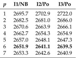
Table2presents a summary of AIC values to compare GINAR(p) with binomial thinning and the I2, I3 thinning operators.

For thinning with I2 and I3, based on AIC values, the models with Poisson innovations are a little better than with NB innovations forp =3 to 7 for I2 and p =4 to 7 for I3. For binomial thinning, based on AIC values, the models with NB innovations are much better than with Poisson innovations. The best models based on AIC values are GINAR(6) models with I2 and I3 thinning operators and Poisson-distributed innovations. They are quite an improvement on INAR(6) with binomial thinning and NB-distributed innovations. Based on the context of the data, thinning operations based on compounding with support on all ofN0instead of{0, 1}are more reasonable.

The I2 and I3 thinning operators account for some conditional heteroscedasticity so that the use of the NB-distributed innovations leads to a flatter log-likelihood over the NB parameters. Hence Poisson distributed innovations are adequate to handle the marginal overdispersion.

Table 2.Ericsson transaction data: AIC values for (5) with three thinning operators and Poisson (Po) and negative binomial (NB) distributions for the innovation. When the autoregressive order reaches 7, there is no improvement in the log-likelihood and the last estimatedαjis close to 0. The AIC values

are based on (10) withistart=8. The AIC values for the best models for each of I1,I2,I3 are boldfaced.

Forp=1 and 2, the AIC values for I2/NB are 2694.6 and 2679.4 respectively, and for I3/NB they are 2690.5 and 2677.1 respectively. For largerp, there is enough conditional heterscedasticity from the thinning operators and NB innovations did not lead to improved AIC values over Poisson innovations.

p I1/NB I2/Po I3/Po

1 2695.7 2702.9 2722.0 2 2682.5 2681.0 2686.0 3 2670.6 2663.9 2666.1 4 2662.7 2654.3 2654.9 5 2657.0 2648.1 2647.3 6 2651.9 2641.1 2639.5 7 2653.3 2642.6 2640.9

We next compare AIC values with other models that have been used for this data set. Table 4.4 and Example 4.2.4 ofWeiß(2018) have values of maximized log conditional likelihoods at the CML estimates for INGARCH(1,1) models with Poisson, NB and generalized Poisson innovations. The use of NB and generalized Poisson distributions lead to much better fitting models with AIC values in the range 2662 to 2666. With a further adjustment for starting in the eighth observation in the conditional log-likelihood, the AIC values are comparable with those in Table2.

With also compare with the Poisson autoregression or INGARCH models inFokianos et al.(2009). The models are conditional Poisson with a latent mean process{Λt}, where[Yt|Λs =λs :s≤t,Ys = ys:s<t]∼Poisson(λt)with

or

λt= (b0+b1exp{−γλt−12 })λt−1+b2yt−1.

As inFokianos et al.(2009), we start the latent process withλ0=0. There is some sensitivity to the starting valuey0but we get similar maximum likelihood parameter estimates when startingy0at the sample mean. When evaluating AIC values withistart =8 are between 2847 and 2849 for these two models and correspond roughly to the AIC value for INGARCH(1,1) with Poisson innovations inWeiß(2018).

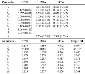
Table3has (a) CML estimates for the GINAR(6) models with I1, I2 and I3 thinning operators, and (b) model-based moments and acf’s from these models to compare with the empirical values. The comparison with empirical values provides a simple goodness-of-fit procedure; in this case, it shows that the fit from GINAR(6) with binomial thinning is a worse fit.

Based on the parameter estimates in this table, and the last 6 values in the data series: (y460,y459,y458,y457,y456,y455) = (3, 9, 29, 18, 20, 7), we can estimate the conditional mean ˆµcond, conditional variance ˆσ_cond2 and central 50% and 80% intervals from estimated pmf:

fYn+1|Yn,...,Yn−5(·|yn, . . . ,yn−5; ˆα1, . . . , ˆα6, ˆθinnov). These are summarized below.

• I1 (binomial thinning): ˆµcond=11.62, ˆσ_cond2 =25.66,[7, 12]with probability content 0.52;[5, 16]

with probability content 0.82;

• I2: ˆµcond = 12.20, ˆσ_cond2 = 30.31, [7, 14]with probability content 0.56; [5, 18]with probability

content 0.82;

• I3: ˆµcond = 12.20, ˆσ_cond2 = 30.92, [7, 13]with probability content 0.51; [5, 18]with probability

content 0.82.

For binomial thinning, the point and interval predictions are smaller and shorter. Please note that these prediction intervals would not be possible with estimation based on conditional least squares or the method of moments.

Table 3. Ericsson transaction data: CML parameter estimates and corresponding SEs for GINAR(6) with I1, I2 and I3 thinning; also model-based summary statistics, to compare with empirical.

Parameter I1/NB I2/Po I3/Po

ˆ

γ 0.533 (0.036) 2.321 (0.333)

ˆ

α1 0.172 (0.037) 0.187 (0.047) 0.194 (0.047) ˆ

α2 0.057 (0.037) 0.068 (0.048) 0.071 (0.047) ˆ

α3 0.086 (0.036) 0.109 (0.049) 0.109 (0.047) ˆ

α4 0.086 (0.037) 0.116 (0.048) 0.117 (0.047) ˆ

α5 0.093 (0.038) 0.104 (0.050) 0.109 (0.047) ˆ

α6 0.105 (0.038) 0.142 (0.048) 0.146 (0.047) ˆ

ϑ 1.068 (0.125)

ˆ

ξ 3.717 (0.509)

ˆ

λ 2.704 (0.538) 2.507 (0.531)

Summary I1/NB I2/Po I3/Po Empirical

ˆ

µY 9.879 9.889 9.892 9.909

ˆ

σ_Y2 27.460 30.070 31.707 32.837

ˆ

ρ1 0.257 0.350 0.374 0.405

ˆ

ρ2 0.176 0.278 0.302 0.340

ˆ

ρ3 0.189 0.297 0.317 0.372

ˆ

ρ4 0.193 0.305 0.326 0.377

ˆ

ρ5 0.201 0.302 0.326 0.358

ˆ

ρ6 0.205 0.321 0.343 0.352

ˆ

6.2. Meningococcal Disease Data

The data set comes from the German national surveillance system for notifiable diseases, administered by the Robert Koch Institute. The time series consists of weekly numbers of meningococcal disease cases in Germany for the years 2001–2006 and the sample size isn = 312. InPedeli et al.(2015), INAR(p) models are fitted with approximate likelihood based on a saddlepoint approximation. There is a seasonal pattern over the year and sinusoidal terms were used as covariates in the mean parameter of the innovations as indicated in Section5.

We fit several GINAR(p) models with I2 and I3 thinning in addition to binomial thinning, using the numerical techniques in the preceding sections. The primary sinusoidal termsxt1=sin(2πt/52)

andxt2=cos(2πt/52). As indicated inPedeli et al.(2015), the addition of additional harmonic terms

xt3=sin(4πt/52)andxt4=cos(4πt/52)do not lead to improvements based on AIC; the estimates

of the corresponding β regression parameters are at least 10 times smaller than those for xt1,xt2.

The autoregressive order started at 1 and increased to a valuepmaxso that the last ˆαjwas close to 0 and the negative log-likelihood value was not improving.

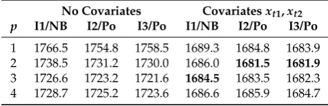
Table4has some AIC values, based onistart =5 in (10). For thinning with I2 and I3, based on AIC values, the models with Poisson innovations are a little better than those with NB innovations for p=2, 3, 4. For binomial thinning, based on AIC values, the models with NB innovations are much better than those with Poisson innovations.

As in the Section 6.1, the I2 and I3 thinning operators account for some conditional heteroscedasticity so that the use of the NB-distributed innovations leads to a flatter log-likelihood over the NB parameters.

Overall, from Table4, the GINAR(2) models with I2 or I3 thinning, Poisson-distributed innovations andxt1,xt2as covariates provide the best models. The best AIC values from GINAR(p) with I2 and I3 thinning are smaller than the best AIC values in Pedeli et al.(2015) (based on binomial thinning).

Table 4. Meningococcal disease data: AIC values for (5) with three thinning operators and Poisson (Po) and negative binomial (NB) distributions for the innovation. The AIC values are based on (10) withistart=5. The AIC values of the best models for each of I1,I2,I3 are boldfaced. The covariates are

xt1=sin(2πt/52)andxt2=cos(2πt/52).

No Covariates Covariatesxt1,xt2 p I1/NB I2/Po I3/Po I1/NB I2/Po I3/Po

1 1766.5 1754.8 1758.5 1689.3 1684.8 1683.9 2 1738.5 1731.2 1730.0 1686.0 1681.5 1681.9 3 1726.6 1723.2 1721.6 1684.5 1683.5 1682.3 4 1728.7 1725.2 1723.6 1686.6 1685.9 1684.7

7. Discussion

We showed how GINAR(p) count time series models can be estimated using numerical maximum likelihood. This allows for sensitivity analysis to model assumptions that is not possible with the estimation methods of conditional least squares and the method of moments.

Future research includes the use of the thinning operators in Definition3in other applications, as well as derivations of other families of self-generalized random variables satisfying Definition2.

Where researchers have been using binomial thinning in count time series models, we recommend the replacement with more general thinning operators that satisfy the self-generalized properties. These operators are more interpretable when the survivor interpretation for binomial thinning does not apply. The examples in this paper show that better fitting models can be obtained.

Funding:This research was funded by NSERC Discovery Grant 8698.

Acknowledgments:Thanks to Konstantinos Fokianos for providing the data sets. Thanks to the referees for their constructive suggestions to improve the presentation.

Conflicts of Interest:The author declares no conflict of interest.

References

Al-Osh, Mohamed A., and Emad-Eldin A. A. Aly. 1992. First order autoregressive time-series with negative binomial and geometric marginals. Communications in Statistics—Theory and Methods21: 2483–92. [CrossRef] Aly, Emad-Eldin A. A., and Nadjib Bouzar. 1994. Explicit stationary distributions for some galton-watson

processes with immigration. Communications in Statistics—Stochastic Models10: 499–517. [CrossRef] Aly, Emad-Eldin A. A., and Nadjib Bouzar. 2019. Expectation thinning operators based on linear fractional

probability generating functions.Journal of the Indian Society for Probability and Statistics20: 89–107. [CrossRef] Alzaid, Abdulhamid A., and Mohamed A. Al-Osh. 1993. Some autoregressive moving average processes with generalized Poisson marginal distributions. Annals of the Institute of Statistical Mathematics45: 223–32. [CrossRef]

Brännäs, Kurt, and A. M. M. Shahiduzzaman Quoreshi. 2010. Integer-valued moving average modelling of the number of transactions in stocks. Applied Financial Economics20: 1429–40. [CrossRef]

Davies, Robert B. 1973. Numerical inversion of a characteristic function. Biometrika60: 415–17. [CrossRef] Davis, Richard A., Scott H. Holan, Robert Lund, and Nalini Ravishanker. 2015. Handbook of Discrete-Valued Time

Series. Boca Raton: Chapman & Hall/CRC.

Du, Jin-Guan, and Yuan Li. 1991. The integer-valued autoregressive (INAR(p)) model. Journal of Time Series

Analysis12: 129–42.

Fokianos, Konstantinos, Anders Rahbek, and Dag Tjostheim. 2009. Poisson autoregression. Journal of the American

Statistical Association104: 1430–39. [CrossRef]

Gauthier, Geneviève, and Alain Latour. 1994. Convergence forte des estimateurs des paramètres d’un processus GENAR(p). Ann. Sci. Math. Québec18: 49–71.

Joe, Harry. 1996. Time series models with univariate margins in the convolution-closed infinitely divisible class.

Journal of Applied Probability33: 664–77. [CrossRef]

Joe, Harry. 1997. Multivariate Models and Dependence Concepts. London: Chapman & Hall.

Joe, Harry. 2015. Markov count time series models with covariates. InHandbook of Discrete-Valued Time Series. Edited by Richard A. Davis, Scott H. Holan, Robert Lund and Nalini Ravishanker. Boca Raton: Chapman & Hall/CRC, chp. 2, pp. 29–49.

Lu, Yang. 2018. Probabilistic Forecasting in Higher-Order INAR(p) Models. MPRA Paper 83682, Munich: University Library of Munich.

McKenzie, Ed. 1986. Autoregressive moving-average processes with negative-binomial and geometric marginal distributions.Advances in Applied Probability18: 679–705. [CrossRef]

McKenzie, Ed. 1987. Innovation distributions for gamma and negative binomial autoregressions. Scandinavian

Journal of Statistics14: 79–85.

Pedeli, Xanthi, Anthony C. Davison, and Konstantinos Fokianos. 2015. Likelihood estimation for the inar(p) model by saddlepoint approximation. Journal of the American Statistical Association110: 1229–38. [CrossRef] Weiß, Christian H. 2018. An Introduction to Discrete-Valued Time Series. Hoboken: Wiley.

Zhu, Rong, and Harry Joe. 2003. A new type of discrete self-decomposability and its application to continuous-time Markov processes for modeling count data time series.Stochastic Models19: 235–54. [CrossRef]

Zhu, Rong, and Harry Joe. 2010a. Count data time series models based on expectation thinning. Stochastic

Models26: 431–62. [CrossRef]

Zhu, Rong, and Harry Joe. 2010b. Negative binomial time series models based on expectation thinning operators.

Journal of Statistical Planning and Inference140: 1874–88. [CrossRef]

c